
Page 60
3
Statistical Approaches to Analysis of Small ClinicalTrials
A necessary companion to well-designed clinical trial is its appropriate statistical analysis. Assuming that a clinical trial will produce data that could reveal differences in effects between two or more interventions, statistical analyses are used to determine whether such differences are real or are due to chance. Data analysis for small clinical trials in particular must be focused. In the context of a small clinical trial, it is especially important for researchers to make a clear distinction between preliminary evidence and confirmatory data analysis. When the sample population is small, it is important to gather considerable preliminary evidence on related subjects before the trial is conducted to define the size needed to determine a critical effect. It may be that statistical hypothesis testing is premature. Thus, testing of a null hypothesis might be particularly challenging in the context of a small clinical trial. Thus, in some cases it might be important to focus on evidence rather than to test a hypothesis (Royall, 1997). This is because a small clinical trial is less likely to be self-contained, providing all of the necessary evidence to effectively test a particular hypothesis. Instead, it might be necessary to summarize all of the evidence from the trial and combine it with other evidence available from other trials or laboratory studies. A single large clinical trial is often insufficient to answer a biomedical research question, and it is even more unlikely that a single small clinical trial can do so. Thus, analyses of data must consider the limitations of the
Page 61
BOX 3-1Some Statistical Approaches to Analysis of Small Clinical Trials
Sequential analysis Hierarchical models Bayesian analysis Decision analysis Statistical prediction Meta-analysis and other alternatives Risk-based allocation |
data at hand and their context in comparison with those of other similar or related studies.
Since data analysis for small clinical trials inevitably involves a number of assumptions, it is logical that several different statistical analysis be conducted. If these analysis give consistent results under different assumptions, one can be more confident that the results are not due to unwarranted assumptions. In general, certain types of analysis (see Box 3-1) are more amenable to small studies. Each is briefly described in the sections that follow.
SEQUENTIAL ANALYSIS
Sequential analysis refers to an analysis of the data as they accumulate, with a view toward stopping the study as soon as the results become statistically compelling. This is in contrast to a sequential design (see Chapter 2), in which the probability that a participant is assigned to a particular intervention is changed depending on the accumulating results. In sequential analysis the probabilty of assignment to an intervention is constant across the study.
Sequential analysis methods were first used in the context of industrial quality control in the late 1920s (Dodge and Romig, 1929). The use of sequential analysis in clinical trials has been extensively described by Armitage (1975), Heitjan (1997), and Whitehead (1999). Briefly, the data are analyzed as the results for each participant are obtained. After each observation, the decision is made to (1) continue the study by enrolling additional participants, (2) stop the study with the conclusion that there is a statistically significant difference between the treatments, or (3) stop the study and conclude that there is not a statistically significant difference between the
Page 62
interventions. The boundaries for the decision-making process are constructed by using considerations of power and size needed to determine an effect size similar to those used to determine sample size (see, for example Whitehead [1999]). Commercially available software can be used to construct the boundaries.
In sequential analysis, the final sample size is not known at the beginning of the study. On average, sequential analysis will lead to a smaller average sample size than that in an equivalently powered study with a fixed-sample-size design. This is a major advantage to sequential analysis and is a reason that it should be given consideration when one is planning and analyzing a small clinical trial. For example, take the case study of sickle cell disease introduced in Chapter 1 and consider the analysis of the clinical design problem introduced in Box 1-4 as an example of sequential analysis ( Box 3-2).
Data from a clinical trial accumulate gradually over a period of time that can extend to months or even years. Thus, results for patients recruited early in the study are available for interpretation while patients are still being recruited and allocated to treatment. This feature allows the emerging evidence to be used to decide when to stop the study. In particular, it may be desirable to stop the study if a clear treatment difference is apparent, thereby avoiding the allocation of further patients to the less successful therapy. Investigators may also want to stop a study that no longer has much chance of demonstrating a treatment difference (Whitehead, 1992, 1997).
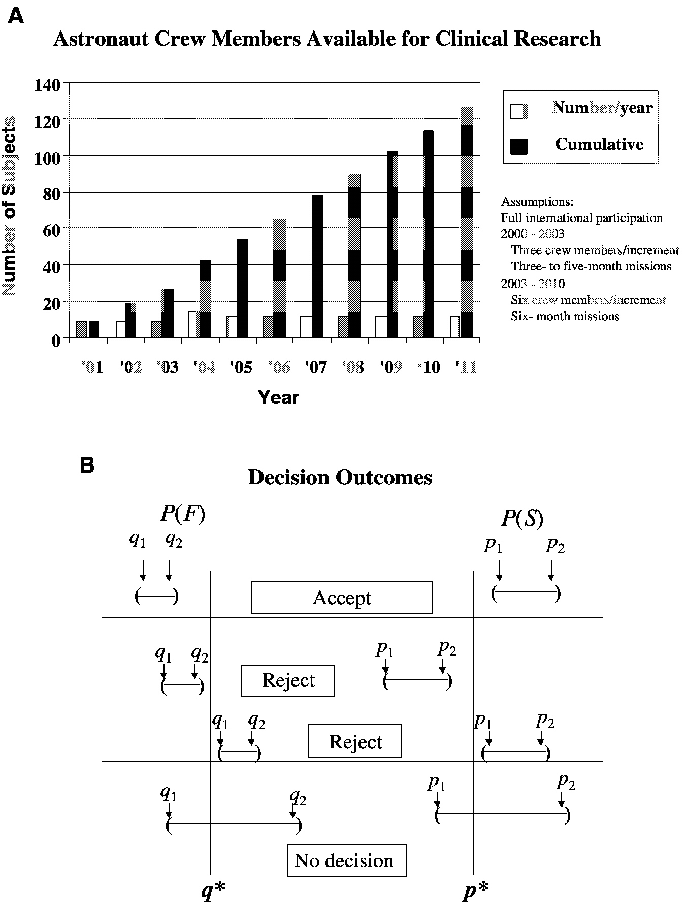
For example, consider the analysis of an intervention (countermeasure) to prevent the loss of bone mineral density in sequentially treated groups of astronauts resulting from their exposure to microgravity during space travel ( Figure 3-1). The performance index is the bone mineral density (in grams per square centimeter) of the calcaneus. S refers to success, where p is the probability of success and p* is the cumulative mean. F refers to failure, where q is the probability of failure and q* is the cumulative mean. The confidence intervals for p and q are obtained after each space mission, that is, for p, (P1, P2), and for q, (q1, q2). The sequential accumulation of data then allows one to accept the countermeasure if p1 is greater than p* and q2 is less than q* or reject the countermeasure if p2 is less than p* or q1 is greater than q*. Performance indices will be acceptable when success S, a gain or mild loss, occurs on at least 75 percent (p* = 0.75) of the cases (astronaut missions) and when F, severe bone mineral density loss, occurs in no more than 5 percent (q* = 0.05) of the cases. Unacceptable performance indices occur with less than a 75 percent success rate or more than a 5 percent failure rate. As the number of performance indices increases, level 1 performance crite-
Page 63
BOX 3-2Clinical Trial for Treatment of Sickle Cell Disease
Sickle Cell disease is a red blood cell (RBC) disorder that affects 1 in 200 African Americans. Fifty percent of individuals living with sickle cell disease die before age 40. The most common complications include stroke, renal failure, and chronic severe pain. Patients who have a stroke are predisposed to having another one. Mixed donor and host stem cell chimerism (e.g., the recipient patient has stem cells of her or his own origin and also those from the transplant donor) is curative for sickle cell disease. Only 20 percent of donor RBC production (and 80 percent of recipient RBC production) is required to cure the abnormality. Conditioning of the recipient is required for the transplanted bone marrow stem cells to become established. The degree of HLA (human leukocyte antigen) mismatch as well as the sensitization state (i.e., chronic transfusion immunizes the recipient) influences how much conditioning is required to establish 20 percent donor chimerism. In patients who have an HLA-identical donor and who have not been heavily transfused, 200 centigrays (cGy) of total body irradiation (TBI) is sufficient to establish donor engraftment (establish a cure). This dose of irradiation has been shown to be well tolerated. In heavily transfused recipients who are HLA mismatched, more conditioning will probably be required. The optimal dose of TBI for this cohort has not been established. The focus of this study is to establish the optimum dose of TBI to achieve 20 percent donor cells (chimerism) in patients enrolled in the protocol. How many patients must be enrolled per cohort to obtain durable bone marrow stem cell establishment (engraftment)? Patients are monitored monthly for the level of donor chimerism. Engraftment can be considered durable if 20 percent donor chimerism is present at ≥6 months. When can TBI dose escalation be implemented? How many patients are required per group before an increase in dose can be made?
One traditional approach to this problem is to identify an acceptable engraftment rate and to then identify the number of subjects required to ensure that the confidence interval for the true proportion is sufficiently narrow to be protective of human health. For example, if the desired engraftment rate is 95 percent, 19 subjects will provide a 95 percent confidence interval with a width of 10 percent (i.e., 0.85 to 1.00). If for a particular application, this interval is too wide, a width of 5 percent can be obtained with 73 subjects (0.90 to 1.00). On the basis of these results, should 73 subjects be required for each TBI dose group? Is a total of 292 patients really needed for all dose groups? The answer is that a much smaller total number of patients is required by invoking a simple sequential testing strategy. For example, assume that the study begins with three patients in the lowest-dose group and it is observed that none of the patients are cured. On the basis of a binomial distribution and by use of a target engraftment proportion of 0.95, the probability that zero of three engraftments will be established when the true population |
Page 64
|
proportion is 0.95 is approximately 1 in 10,000. Similarly, the cumulative probability of one or fewer cures is less than 15 percent. As such, after only three patients are tested, considerable information regarding whether the true cure rate is 95 percent or more is already available. Following this simple sequential strategy, one would test each dose (beginning with the lowest dose) with a small number of patients (e.g., three patients) and increase to the next dose level if the results of the screening trial indicate that the probability of cure for the targeted proportion (e.g., 0.95 percent) is small. In the current example, one would clearly increase the dose if zero of three patients was cured and would most likely increase the dose to the next level even if one or two patients were cured. If, in this example, all three patients engrafted, one would then test either 19 or 73 patients (depending on the desired width of the confidence interval) and determine a confidence interval for the true engraftment rate with the desired level of precision. If the upper confidence limit is less than the targeted engraftment rate, then one would proceed to the next highest TBI dose level and repeat the test. |
ria can be set; for example, S is equal to a gain or no worse than 1 percent loss of bone mineral density relative to that at baseline. Indeterminate (I) is equal to a moderate loss of 1 to 2 percent from that at the baseline. F is equal to the severe loss of 2 percent or more from that at the baseline (Feiveson, 2000). See Box 1-2 for an alternate design discussion of this case study.
The use of study stopping (cessation) rules that are based on successive examinations of accumulating data may cause difficulties because of the need to reconcile such stopping rules with the standard approach to statistical analysis used for the analysis of data from most clinical trials. This standard approach is known as the “frequentist approach.” In this approach the analysis takes a form that is dependent on the study design. When such analyses assume a design in which all data are simultaneously available, it is called a “fixed-sample analysis.” If the data from a clinical trial are not examined until the end of the study, then a fixed-sample analysis is valid. In comparison, if the data are examined in a way that might lead to early cessation of the study or to some other change of design, then a fixed-sample analysis will not be valid. The lack of validity is a matter of degree: if early cessation or a change of design is an extremely remote possibility, then fixed-sample methods will be approximately valid (Whitehead, 1992, 1997).
For example, in a randomized clinical trial for investigation of the effect of a selenium nutritional supplement on the prevention of skin cancer, it is determined that plasma selenium levels are not rising as expected in some patients in the supplemented group, indicating a possible noncompliance problem. In this case, the failure of some subjects to receive the prescribed amount of selenium supplement would have led to a loss of power to detect a significant benefit, if one was present. One could then initiate a prestudy
Page 65
~ enlarge ~
FIGURE 3-1 Parameters for a clinical trial with a sequential design for prevention of loss of bone mineral density in astronauts. A. Group sample sizes available for clinical study. B. Establishment of repeated confidence intervals for a clinical intervention for prevention of loss of bone mineral density for determination of the success (S) or failure (F) of the intervention.
SOURCE: Feiveson (2000).
Page 66
BOX 3-3Sequential Testing with Limited Resources
As an illustration of sequential testing in small clinical studies, consider the innovative approach to forensic drug testing proposed by Hedayat, Izenman, and Zhang (1996). Suppose that N units such as pills or tablets or squares of lysergic acid diethylamide (LSD) are obtained during an arrest and one would like to determine the minimal number that would have to be screened to state with 95 percent confidence that at least N1 of the total N samples will be positive. To solve the problem, define m as the expected number of negative units in the initial random sample of n units and X as the observed number of negative units in a sample of size n. Typically, the forensic scientist assumes that m is equal to 0, n samples are collected, and the actual number of negative samples (X) is determined. Next, define k as the minimum number of positive drug samples that are needed to achieve a conviction in the case. One wishes to test with a confidence of 100(1 − α, where α is the probability of committing a type 1 error) percent that N1 ≥ k. The question is: what is the smallest sample size n needed? Hedayat and co-workers showed that the problem can be described in terms of the inequality maxN1<kProb[X ≤ m | N1] ≤ α, which is equivalent to maxN1≤k−1 Prob[X ≤ m | N1] ≤ α, and is satisfied by Prob[X ≤ m | N1 = k − 1] ≤ α. This is a cumulative probability of the hypergeometric distribution, that can be expressed as 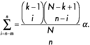
~ enlarge ~ |
treatment period in which potential noncompliers could be identified and eliminated from the study before randomization (Jennison and Turnbull, 1983).
Another reason for early examination of study results is to check the assumptions made when designing the trial. For example, in an experiment where the primary response variable is quantitative, the sample size is often set assuming this variable to be normally distributed with a certain variance. For binary response data, sample size calculations rely on an assumed value for the background incidence rate; for time-to-event data when individuals enter the trial at staggered intervals, an estimate of the subject accrual rate is important in determining the appropriate accrual period. An early interim
Page 67
|
For example, assume that the total number of units under investigation is 150 and suppose that one wants to claim with 95 percent confidence that the number of positive units, N1, is at least 135. If one assumes that there will be no negative units in the initial sample (i.e., m = 0) then one can begin with an initial sample of 25, using the inequality given above. The investigators draw a random sample of 25, and if no negative units are found, the investigators can conclude with 95 percent confidence that the total number of positive units (N1) is greater than 135. Note that if one actually observes X to be equal to 1 negative unit, one then can determine what value of N1 is feasible or recompute n. For example, say that one observes X is equal to 2 negative units among 25 initial samples. With 95 percent confidence one can claim that k equal to 118 positive units will be found. Alternatively, if one requires N1 to be ≥ 135 positive units, one can increase n to 61 samples by drawing an additional 61 - 25 = 36 random samples. A useful example in clinical trials is the comparison of a new drug with a standard drug for the treatment of a rare disease. For example, it may be known that the rate of response to an existing drug is 80 percent; however, the drug has serious side effects. A new drug without the side effect profile of the old drug has been developed, but it is not known whether it is equally efficacious. Power computations revealed that 150 subjects are required to document that the response rate is at least 90 percent with 95 percent confidence (i.e., at least 135 of 150 patients respond). Unfortunately, 150 subjects are not available. Using the strategy developed by Hedayat and colleagues (1996), one can examine 25 patients, and if they all respond, then one can conclude with 95 percent confidence that the total number of responders is at least 135 among the 150 patients that the investigators would have liked to test. There are numerous applications of this type of sequential testing strategy in small clinical trials. |
analysis can reveal inaccurate assumptions in time for adjustments to be made to the design (Jennison and Turnbull, 1983).
Sequential methods typically lead to savings in sample size, time, and cost compared with those for standard fixed-sample procedures ( Box 3-3). However, continuous monitoring is not always practical.
HIERARCHICAL MODELS
Hierarchical models can be quite useful in the context of small clinical trials in two regards. First, hierarchical models provide a natural framework for combining information from a series of small clinical trials conducted
Page 68
within ecological units (e.g., space missions or clinics). In the case where the data are complete, in which the same response measure is available for each individual, hierarchical models provide a more rigorous solution than meta-analysis, in that there is no reason to use effect magnitudes as the unit of observation. Note, however, that a price must be paid (i.e., the total sample size must be increased) to reconstruct a larger trial out of a series of smaller trials. Second, hierarchical models also provide a foundation for analysis of longitudinal studies, which are necessary for increasing the power of research involving small clinical trials. By repeatedly obtaining data for the same subject over time as part of a study of a single treatment or a crossover study, the total number of subjects required in the trial is reduced. The reduction in the sample size number is proportional to the degree of independence of the repeated measurements.
A common theme in medical research is two-stage sampling, that is, sampling of responses within experimental units (e.g., patients) and sampling of experimental units within populations. For example, in prospective longitudinal studies patients are repeatedly sampled and assessed in terms of a variety of endpoints such as mental and physical levels of functioning or in terms of the response of one or more biological systems to one or more forms of treatment. These patients are in turn sampled from a population, often stratified on the basis of treatment delivery, for example, in a clinic, in a hospital, or during space missions. Like all biological and behavioral characteristics, the outcome measures exhibit individual differences. Investigators should be interested in not only the mean response pattern but also the distribution of these response patterns (e.g., time trends) in the population of patients. One can then address the number or proportion of patients who are functioning more or less positively at a specific rate. One can then describe the treatment-outcome relationship not as a fixed law but as a family of laws, the parameters of which describe the individual biobehavioral tendencies of the subjects in the population (Bock, 1983). This view of biological and behavioral research may lead to Bayesian methods of data analysis. The relevant distributions exist objectively and can be investigated empirically.
In medical research, a typical example of two-stage sampling is the longitudinal clinical trial, in which patients are randomly assigned to different treatments and are repeatedly evaluated over the course of the study. Despite recent advances in statistical methods for longitudinal research, the cost of medical research is not always commensurate with the quality of the analyses. Reports of such studies often consist of little more than an end-
Page 69
point analysis in which measurements only for those participants who have completed the study are considered in the analysis or the last available measurement for each participant is carried forward as if all participants had, in fact, completed the study. In the first example of a “completer- only” analysis, the available sample at the end of the study may have little similarity to the sample initially randomized. There is some improvement in the case of carrying the last observation forward. However, participants treated in the analysis as if they have had identical exposures to the drug may have quite different exposures in reality or their experiences while receiving the drug may be complicated by other factors that led to their withdrawal from the study but that are ignored in the analysis. Both cases lead to dramatic losses of statistical power since the measurements made on the intermediate occasions are simply discarded. In these studies a review of the typical level of intraindividual variability of responses should raise serious questions regarding reliance on any single measurement.
To illustrate the problem, consider the following example. Suppose a longitudinal randomized clinical trial is conducted to study the effects of a particular therapeutic intervention (countermeasure) on bone mineral density measurements taken at multiple points in time during the course of a space mission. At the end of the study, the data comprise a file of bone mineral density measurements for each patient (astronaut) in each treatment group. In addition to the usual completer or end-point analysis, a data analyst might compute means for each week and might fit separately for each group a linear or curvilinear trend line that shows average bone mineral density loss per week. A more sophisticated analyst might fit the line using some variant of the Potthoff-Roy procedure, although this would require complete and similarly time-structured data for all subjects (Bock, 1979).
Despite the question of whether bone mineral density measurements are related to the ability of an astronaut to function in space, most objectionable is the representation of the mean trend in the population as a biological relationship acting within individual subjects. The analysis might purport that as any astronaut uses a countermeasure he or she will decrease the effect of life in a weightless environment on bone mineral density loss at some fixed rate (e.g., 0.1 percent per week). This is a gross oversimplification. The account is somewhat improved by reporting of mean trends for important subgroups: astronauts of various ages, males and females, and so on. Even then, within such groups some patients will respond more to a given countermeasure, some will respond less, and the responses of others will not change at all. Like all biological characteristics, there are individual differ-
Page 70
ences in response trends. Therefore, both the mean trend and the distribution of trends in the population of patients are of interest. One can then speak of the number or proportion of patients who respond to a clinically acceptable degree and the rates at which their biological status changes over time.
In a longitudinal study, repeated observations are nested within individuals and the hierarchical model is used to incorporate the effects of intrasubject correlation on estimates of uncertainty (i.e., standard errors and confidence intervals) and tests of hypotheses for the fixed effects or structural parameters (e.g., differential treatment efficacy) in the model. Note that hierarchical models are equally useful in the context of clustered data, in which participants are nested within groups (e.g., different studies or space missions), and the sharing of this similar environment induces a correlation among the responses of participants within strata.
Analysis of this type of data (under the assumptions that a subset of the regression parameters has a distribution in the population of participants and that the model residuals have a distribution in the population of responses within participants and also in the population of participants) belongs to the class of statistical analytical models called:
-
mixed model (Elston and Grizzle, 1962; Longford, 1987);
-
regression with randomly dispersed parameters (Rosenberg, 1973);
-
exchangeability between multiple regressions (Lindley and Smith, 1972);
-
two-stage stochastic regression, (Fearn, 1975);
-
James-Stein estimation (James and Stein, 1961);
-
variance component models (Dempster, Rubin, and Tsutakawa, 1981; Harville, 1977);
-
random coefficient models (DeLeeuw and Kreft, 1986);
-
hierarchical linear models (Bryk and Raudenbush, 1987);
-
multilevel models (Goldstein, 1986); and
-
random-effect regression models (Laird and Ware, 1982).
Along with the seminal articles that have described these statistical models, several book-length texts that further describe these methods have been published (Bock, 1989; Bryk and Raudenbush, 1992; Diggle, Liang, and Zeger, 1994; Goldstein, 1995;Jones, 1993; Lindsey, 1993; Longford, 1993). For the most part, these treatments are based on the assumptions that the residual effects are normally distributed with zero means and a covariance
Page 71
BOX 3-4Power Consideration for Space Mission Clinical Trials
A natural application for hierarchical regression models is the problem in which astronauts are nested within space missions and the intervention (e.g., the presence or the absence of a particular countermeasure) is randomly assigned at the level of the space mission. To illustrate the problem, assume that one is interested in detecting a difference of a 0.5 standard deviation unit between control and experimental conditions by a one-tailed test. In addition, assume that five astronauts are available per space mission and that the intraspace mission correlation is 0.2. Assuming a Type I error rate of 5 percent (i.e., 95 percent confidence), how many space missions are required to have 80 percent statistical power of detection of a difference? Using statistical power computations for the clustered t distribution (Hsieh, 1988) one finds that detection of a difference of 0.5 standard deviation unit with 80 percent power would require for each condition (i.e., the control versus the experimental condition) 18 space missions, each with 5 subjects, or a total of 180 astronauts.Note that if the effect size is increased to a difference of 1 standard deviation unit, which may be acceptable for bone mineral density measurement data, the number of space missions is reduced to 5 per condition, for a total of 50 astronauts. In a longitudinal study (i.e., repeated evaluation of astronauts during their tour of duty), statistical power computations become more complex because they can involve both random effects and residual autocorrelations. (The interested reader is referred to the paper by Hedeker, Gibbons, and Waternaux [1999]). |
matrix in all participants, and that the random effects are normally distributed with zero means and covariance matrix. Recent review articles summarize the use of hierarchical models in biostatistics and health services research (Gibbons, 2000; Gibbons and Hedeker, 2000). Some statistical details of the general linear hierarchical regression model are provided in Appendix A. The case study presented in Box 3-4 provides an example of how hierarchical models can be used to aid in the design and analysis of small clinical trials.
BAYESIAN ANALYSIS
The majority of statistical techniques that clinical investigators encounter are of the frequentist school and are characterized by significance levels, confidence intervals, and concern over the bias of estimates (Jennison and Turnbull, 1983). The Bayesian philosophy of statistical inference however is fundamentally different from that underlying the frequentist approach (Malakoff, 1999; Thall, 2000). In certain types of investigations Bayesian
Page 72
analysis can lead to practical methods that are similar to those used by statisticians who use the frequentist approach.
The Bayesian approach has a subjective element. It focuses on an unknown parameter value q, which measures the effect of the experimental treatment. Before designing a study or collecting any data, the investigator acquires all available information about the activities of both the experimental and the control treatments. This provides some information about the possible value of θ.
The Bayesian approach is based on the supposition that the investigator's opinion can be expressed in the form of a value for P(θ ≤ x) for every x between − ∞ and ∞. Here P(θ ≤ x) represents the probability that θ is less than or equal to x. The probability is not frequentist: it does not represent the proportion of times that θ is less than or equal to x. Instead, P(θ ≤ x) represents how likely the investigator thinks it to be that θ is less than or equal to x. The investigator is allowed to think only in terms of functions P(θ ≤ x) which rise from 0 at x = − ∞ to 1 at x = ∞. Thus P(θ ≤ x) defines a probability distribution for θ1, which will be called the subjective distribution of θ. Notice how deep the division between the frequentist and the Bayesian goes: even the notion of probability receives a different interpretation (Jennison and Turnbull, 1983, p. 203).
Thus, before the investigator has observed any data, a subjective distribution of θ can be formulated from the experiences and knowledge gained by others. At this stage, the subjective distribution can be called the prior distribution of θ. After data are collected, these will influence and change opinions about θ. The assessment of where q lies may change (reflected by a change in the location of the subjective distribution), and uncertainty about its value should decrease (reflected by a decrease in the spread of this subjective distribution). The combination of observed data and prior opinion is governed by Bayes's theorem, which provides an automatic update of the investigator's subjective opinion. The theorem then specifies a new subjective distribution for θ, called a posterior distribution (Jennison and Turnbull, 1983).
The attraction of the Bayesian approach lies in its simplicity of concept and the directness of its conclusions. Its flexibility and lack of concern for interim inspections are especially valuable in sequential clinical trials. The main problem with the Bayesian approach, however, lies in the idea of a subjective distribution.
Subjective opinions are a legitimate part of personal inferences. A small investigating team might be in sufficient agreement to share the same prior distribution but it is less likely that all members of the team will hold the same prior opinions and some members will be reluctant to accept an analysis based in part on opinions that they do not share. An alternative possibility is for investi-
Page 73
gators to adopt a prior distribution representing only vague subjective opinion, which is quickly overwhelmed by information from the data. The latter suggestion leads to analyses which are similar to frequentist inferences, but it would appear to lose the spirit of the Bayesian approach. If the prior distribution is not a true representation of subjective opinion then neither is the posterior (Jennison and Turnbull, 1983, p. 204).
More generally, the Bayesian approach has the following advantages:
-
Problem formulation. Many problems, such as inferences or decision making based on small amounts of data, are easy to formulate and solve by Bayesian methods.
-
Sequential analysis. Because the posterior distribution can be updated repeatedly, using each successive posterior distribution as the prior distribution for the next update, it is the natural paradigm for sequential decision making.
-
Meta-analysis. Bayesian hierarchical models provide a natural framework for combining information from different sources. This is often referred to as “meta-analysis” in the context of clinical trials, but the methods are quite broadly applicable.
-
Prediction. An especially useful tool is the predictive probability of a future event. This allows one to make statements such as “Given that an astronaut has not suffered bone mineral density loss during the first year of a 2-year space mission, the probability that he or she will suffer bone mineral density loss during the second year is 25 percent.”
-
Communication. Bayesian models, methods, and inferences are often easier to communicate to nonstatisticians. This is because most people think and behave like Bayesians, whether or not they understand or are even aware of the formal paradigm. The posterior distribution provides a framework for describing and communicating one's conclusions in a variety of ways that make sense to nonstatisticians. Although the details are not presented here, Bayesian methods (Thall, 2000; Thall and Sung, 1998; Thall and Russell, 1998; Thall, Simon, and Estey, 1995; Thall, Simon, and Shen, 2000; White-head and Brunier, 1995) can be applied in most of the design and analysis situations described in this report and in many cases will be extremely useful for the analysis of results of small clinical trials.
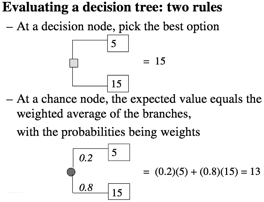
DECISION ANALYSIS
Decision analysis is a modeling technique that systematically considers all possible management options for a problem (Hillner and Centor, 1987). It uses probabilities and utilities to explicitly define decisions. The computa-
Page 74
tional methods allow one to evaluate the importance of any variable in the decision-masking process. Sensitivity analysis describes the process of recalculating the analysis as one changes a variable through a series of plausible values. The steps to be taken in decision analysis are outlined in Table 3-1.
As mentioned in Chapter 2, one can use decision analysis as an aid in the experimental design process. If one models a clinical situation a priori, one can test the importance of a single value in making the decision in question. Performance of a sensitivity analysis before a study is designed to provide an understanding of the influence of a given value on the decision. Such analyses can determine the best use of a small clinical trial. This pre-analysis allows one to focus data collection on important variables (see Box 3-5).
The other major advantage of decision analysis occurs after data collection. If one assumes that the sample size is inadequate and therefore that the confidence intervals on the effect in question are wide, one may still have a clinical situation for which a decision is required. One might have to make decisions under conditions of uncertainty, despite a desire to increase the certainty. The use of decision analysis can make explicit the uncertain decision, even informing the level of confidence in the decision. A 1990 Institute of Medicine report states: it is this flexibility of decision analysis that gives it the potential to help set priorities for clinical investigation and effective transfer of research findings to clinical practice (Institute of Medicine, 1990). The formulation of a decision analytical model helps investigators consider which health outcomes are important and how important they are to one another. Decision analysis also facilitates consideration of the potential marginal benefit of a new intervention by forcing comparisons with other alternatives or “fallback positions.” Combining several methodologies, such as
|
Page 75
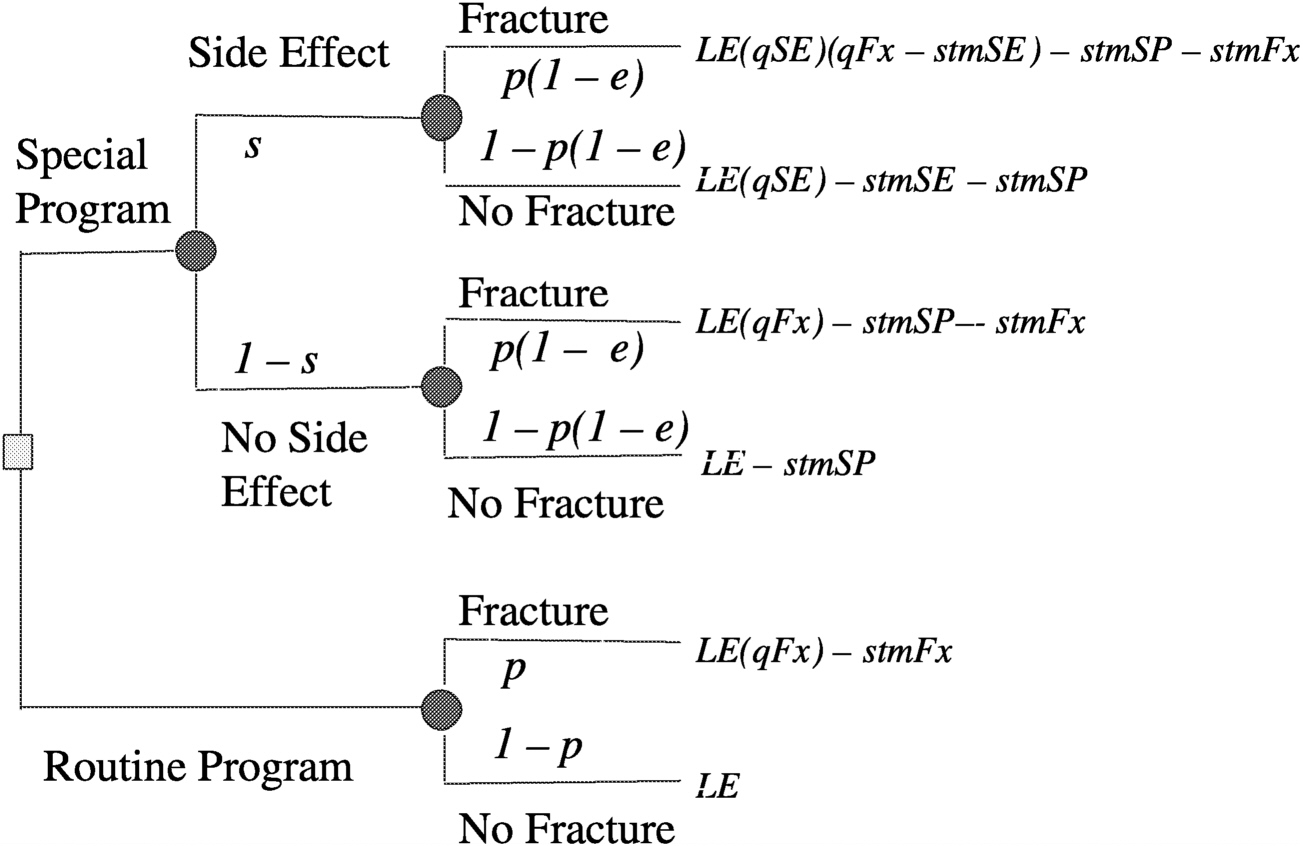
Consider a decision analysis that takes the following into consideration: a long space mission accelerates bone mineral density loss, bone mineral density loss can produce fractures now or in the future, fractures produce disabilities now and disabilities in the future, and a proposed special program may have efficacy in ameliorating bone mineral density loss, but may have side effects. Determine the expectation by evaluating a decision tree (
Figure 3.2). A decision tree can be set up for either a surrogate measure of bone loss (e.g., bone mineral density loss) or for an actual disabling outcome (e.g., bone fracture, as illustrated in
Figure 3.3). Then by making a number of assumptions, such as probability of fracture (p) = 0.2, efficacy of special program (e) = 0.3, probability of side effects (s) = 0.05, quality of life (LT) after fracture (qFx) = 0.85, quality of life (LT) after side effects (qSE) = 0.999, life expectancy of astronaut (LE) = 35 y, where y is years, short-term morbidity fracture (stmFx) = 0.3 y, short-term morbidity side effects (stmSE) = 0.1 y, and short-term morbidity special program (stmSP) = 0.04 y one can assign values at the chance nodes to pick the best option (see
Figure 3.4).
BOX 3-5
Using Decision Analysis to Prevent Osteoporosis in Space
~ enlarge ~
FIGURE 3-2 Decision analysis expectation. SOURCE: Pauker (2000).
Page 76
~ enlarge ~
FIGURE 3-3 Decision tree for preventing osteoporotic fractures in space. SOURCE: Pauker (2000).
~ enlarge ~
FIGURE 3-4 Assigning values at chance nodes to pick the best option (clinical intervention) for preventing osteoporotic fractures in space. SOURCE: Pauker (2000).
Page 77
decision analysis, with a sequential clinical trials approach potentially offers additional improvements in the means of determining the efficacy of a therapeutic intervention in small trial populations.
Although decision analysis does not address the questions raised by small clinical trials, it can allow a better trial design to be used and interpretation of the results of such trials.
-
Decision analytical models can combine data from diverse sources and examine interactions.
-
Decision analytical models are most powerfully used to answer the question “What if?” by sensitivity analyses.
-
Decision analytical models can examine the impact of morbidity and effects on quality of life because they can integrate many attributes in a utility structure.
-
Decision analyses might be used sequentially in small ongoing trials, in which the results for every additional patient might guide the use of the model for subsequent patients.
-
Probability functions such a beta functions can provide such automatic updating of distributions in a model as more patients' experiences are revealed (Pauker, 2000).
STATISTICAL PREDICTION
When the number of control samples is potentially large and the number of experimental samples is small and is obtained sequentially from a series of clusters with small sample sizes (e.g., space missions), traditional comparisons of the aggregate means or medians may be of limited value. In those cases, one can view the problem not as a classical hypothesis testing problem but as a problem of statistical prediction. Conceptualized in that way, the problem is one of deriving a limit or interval on the basis of the control distribution that will include the mean or median for all or a subset of the experimental cluster samples. For example, one may wish to compare the median bone mineral density loss in 5 astronauts in each of five future space missions (i.e., a total of 25 astronauts clustered in groups of 5 each) with the distribution of bone mineral density loss in controls over a similar period of time on Earth or alternatively with that for a control group of astronauts who are in a weightless environment (e.g., the International Space Station) but who are not taking part in a particular countermeasure program. As the number of cluster samples increases, confidence in the deci-
Page 78
sion rule also increases. In the following, a general nonparametric approach to this problem is developed, and its use is illustrated with the problem of testing for bone mineral density loss during space missions. Although more general than parametric alternatives, a loss of statistical power is associated with the nonparametric approach. Parametric alternatives (normal, lognormal, and Poisson distributions) are presented in Appendix A and can be used when the observed data are consistent with one of these distributions.
The prediction problem involves construction of a limit or interval that will contain one or more new measurements drawn from that same distribution with a given level of confidence. As an example, in environmental monitoring problems one may be interested in determining whether a single new measurement (or the mean of n new measurements) obtained from an onsite monitoring location is consistent with background levels as characterized by a series of n measurements obtained from off-site (i.e., background) monitoring locations.
If the new measurement(s) lies within the interval (or below [above] the upper [lower] limit), then one can conclude that the measurement from the on-site monitoring location is consistent with the background measurement and is therefore not affected by activities at the site from which the measurement was obtained. By contrast, if the new measurement(s) lies outside of the interval, one can conclude that it is inconsistent with the background measurement and may potentially have been affected by the activities at the site (e.g., disposal of waste or some industrial process).
One can imagine that as the number of future measurements (i.e., new monitoring locations and number of constituents to be examined) gets large, the prediction interval must expand so that the joint probability of any one of those comparisons by chance done is small, say 5 percent. Of course, this results in a loss of statistical power. To this end, Gibbons (1987b) and Davis and McNichols (1987) (see Gibbons [1994] for a review) suggested that the new measurements be tested sequentially so that a smaller and more environmentally protective limit can be used. The basic idea is that in the presence of an initial value that exceeds the background level in an on-site monitoring location (initial exceedance), another sample for independent verification of the level should be obtained. A true exceedance is indicated only if both the initial level and the verification resample exceed the limit (or are outside the interval). There are many variations of this sequential strategy in which more than one additional sample (resample) may be obtained. The net result is that a much smaller prediction limit can be used sequentially compared with the limit that would be used if the statistical prediction decision was based on the result of a single comparison, leading to a dra-
Page 79
matic increase in statistical power. In fact, this strategy is now used almost exclusively in environmental monitoring programs in the United States (Davis, 1993; Gibbons, 1994, 1996; Environmental Protection Agency, 1992).
This idea can be directly adapted to the problem of loss of bone mineral density in astronauts, particularly with respect to the design and analysis of data from a series of small clinical trials (e.g., space missions, each consisting of a small number of astronauts) and in which a potentially large number of outcomes are simultaneously assessed. To provide a foundation, consider the case in which a study has n control subjects (e.g., astronauts on the International Space Station or in a simulated environment, but without countermeasures) and a series of p replicate experimental cohorts (e.g., space missions), each of size ni (e.g., ni = 5 astronauts in each of p = 5 space missions). The objective is to use the n control measurements to derive an upper (lower) bound for a subset (e.g., 50 percent) of the ni experimental subjects in at least one of the p experimental subject cohorts (e.g., space missions).
Given the previous characterization of the problem and the questionable distributional form of the outcomes of multiple countermeasures, a natural approach to the solution of this problem is to proceed nonparametrically. For a particular outcome (e.g., bone mineral density), define an upper prediction limit as the uth largest control measurement among the n control subjects. If u is equal to n, the prediction limit is the largest control measurement for that particular outcome measure or endpoint. If u is equal to n − 1 then the prediction limit is the second largest control measurement for that outcome measure. A natural advantage of using u < n is that it provides an automatic adjustment for outliers, in that the largest n − u values are removed. Note, however, that the larger the difference between u and n the lower the overall confidence, if everything else is kept equal.
Now consider the experimental subjects. Assume that ni experimental subjects (e.g., astronauts who are subjected to experimental countermeasures) exist in each of p experimental subject cohorts (e.g., space missions). Let si be the number of subjects required to be contained within the interval for cohort i. For example, if ni is equal to 5 and one wishes to have the median value for cohort i be below the upper prediction limit, then si is equal to 3. An effect of the experimental intervention on a particular outcome measure is declared only if the sith largest measurement (e.g., the median) lies outside of the prediction interval (or above [below] the prediction limit in the one-sided case) in all p experimental subject cohorts.
The questions of interest are as follows:
Page 80
1. What is the probability of a chance exceedance in all p experimental subject cohorts for different values of n, u, ni, si, and p?
2. How is this probability affected by various numbers of outcome measures (i.e., k)?
3. What is the power to detect a real difference between control and experimental conditions for a given statistical strategy?
A drawback to this method is that the control group is typically not a concurrent control group. Thus, if other conditions, in addition to the intervention being evaluated, are changed, it will not be possible to determine if the changes are in fact due to the experimental condition.
Specific details regarding implementation of the approach and a general methodology for answering these questions is presented in Appendix A and is illustrated in Box 3-6.
The use of statistical prediction limits described here represents a paradigm shift in the way in which small clinical studies are designed and analyzed. The method involves characterization of the distribution of control measurements and the use of parameters for the control distribution to draw inferences from a series of more limited samples of experimental measurements. This is a classical problem in statistical prediction and departs from the more commonly used paradigm of hypothesis testing. The methodology described here is applicable to virtually any problem in which the number of potential endpoints is large and the number of available subjects is small. In a recent work by Gibbons and colleagues (submitted for publication), a similar approach was developed to compare relatively small numbers of experimental tissues to a larger number of control tissues in terms of potentially thousands of gene expression levels obtained from nucleic acid microarrays. To provide ease of application, they developed a “probability calculator” that computes confidence levels and statistical power for any set of values of n, ni, p, u, i, si, and k. (The probability calculator is freely available at www.uic.edu/labs/biostat/ and is useful for both design and analysis of small clinical studies.)
META-ANALYSIS: SYNTHESIS OF RESULTS OF INDEPENDENT STUDIES
Meta-analysis refers to a set of statistical procedures used to summarize empirical research in the literature ( Table 3-2). Although the concept of combining the results of many studies has its origins in the early 1900s agricultural experiments, Glass in 1976 coined the term to mean “the analysis of
Page 81
BOX 3-6Case Study of Bone Mineral Density Loss During Space Missions
Space travel in low Earth orbit or beyond Earth's orbit exposes individuals (astronauts or cosmonauts) to environmental stresses (e.g., microgravity and cosmic radiation) that, if unabated, could result in radiation-induced physiological damage or marked physiological adaptation (microgravity-induced shifts in calcium and bone metabolism) that could be deleterious or even fatal during space travel, on landing on another planet, or after the return to Earth. Based on the preceding discussion of statistical prediction, one can consider the details of design and analysis of a potential study of bone mineral density loss in astronauts. Assume that there are n control astronauts in either a simulated environment or on the International Space Station not taking part in a countermeasure program, or perhaps serving as matched control astronauts on Earth and ni experimental subjects (e.g., astronauts subjected to experimental countermeasures) in each of p space missions. Let si be the number of subiects required to be contained within the interval for space mission i. For example, if ni is equa to 5 and one wishes to have the median value in space mission i below the upper prediction limit, then si is equal to 3. An effect of the experimental intervention on a particular outcome measure is declared only if the sith largest measurement (e.g., the median) lies outside of the prediction interval (or above [below] the prediction limit in the one-sided case) in all p space missions. Statistical details for both parametric and nonparametric solutions to this problem are presented in Appendix A. Returning to the example, suppose that a series of 20 control astronauts on Earth are monitored for the same period of time that 5 astronauts on a single space mission are evaluated for the effects of a series of countermeasures on bone mineral density loss. The question is whether the countermeasures are sufficient to eliminate the effect of the space mission on bone mineral density loss, such that the bone mineral density measurements for the experimental astronauts are consistent with the bone mineral density measurements for the control astronauts. To this end, consider a comparison of the maximum of 20 control measurements (n = u = 20) with the median far a single space mission (p = 1 ) with ni equal to five experimental astronauts (i.e., si = 3) for a single outcome measure (Case A). Using the previous equations, one obtains an overall confidence level of 99.6 percent, indicating an extremely low probability that the experimental median will be above the largest control bone mineral density measurement by chance alone. One can do better, however. Instead of selecting the most extreme control measurement, take the 18th largest measurement (Case B). In this case, the confidence is 96 percent and one has a more powerful decision rule. Now, consider the effects of multiple endpoints (Case C). With k equal to 10 endpoints and the prediction limit defined as the 18th largest control measurement, the overall confidence level for the experiment is reduced to 68 percent. To counteract this effect (Case D), one can add a second space mission (p = 2), each with ni equal to five astronauts, and the overall confidence is increased back to 96 percent. If one had instead considered p equal to four space missions (Case E), a confidence of 94 percent would be achieved by setting the prediction limit to the 15th largest control measurement, again increasing the statistical power of the decision rule. How does one select from among the various strategies described in the simple example described above? The answer is to select the strategy that has reasonable confidence (i.e., a low rate of false-positive results, e.g., 5 percent) and that has the maximum statistical power for a desired effect size. To this end, one can evaluate the power of the test to detect a true difference between the control group and the experimental group by simulation. |
Page 82
analyses.” Meta-analysis is widely used in education (see Box 3-7), psychology, and the medical sciences (e.g., in evidence-based medicine) and has frequently been used to study the efficacies of different treatments (Hedges and Olkin, 1985).
A meta-analysis can summarize an entire set of research in the literature, a sample from a large population of studies, or some defined subset of studies (e.g., published studies or n-of-1 studies). The degree to which the results of a synthesis can be generalized depends in part on the nature of the set of studies. In general, meta-analysis serves as a useful tool to answer questions for which single trials were underpowered or not designed to address. More specifically, the following are benefits of meta-analysis:
-
It can provide a way to combine the results of studies with different designs (within reason) when similar research questions are of interest.
-
It uses a common outcome metric when studies vary in the ways in which outcomes are measured.
-
It accounts for differences in precision, typically by weighting in proportion to sample size.
-
Its indices are based on sufficient statistics.
-
It can examine between-study differences in results (heterogeneity).
It can examine the relationship of study outcomes to study features (Becker, 2000).
|
Page 83
BOX 3-7Combining n-of-1 Studies in Meta-Analysis: Results from Research in Special Education
Researchers in special education are often concerned with individualized treatments for behavior disorders or with low-incidence disabilities and disorders. Single-case research designs are quite common. Study designs typically involve a baseline period followed by a treatment period and possibly follow-up. Multiple measures are usually obtained from each case during the baseline and treatment. Crossover treatment designs are occasionally used and usually involve only no baseline-treatment cycles. Meta-analysis has been applied since the 1980s to summarize these case-study designs. However, the methods proposed have been controversial and the statistical properties of the methods have not been rigorously studied. Three approaches have been used to measure effects. (1) Single-case effect size. Some researchers have used an index similar to the effect size, computed for n > 1 studies as the standardized difference between group means: 
~ enlarge ~ YÌ„treatment is the subject's mean score during treatment, YÌ„baseline is the mean before treatment, and SY pooled is obtained by pooling intrasubject variation across the two time periods. (2) Percentage of nonoverlapping data index (PND) (Scruggs, Mastropieri, and Castro, 1987). The percentage of nonoverlapping data index is also based on the idea of examining the data from the baseline and treatment periods of the case study. The index is the percentage of datum values observed during treatment that exceed the highest baseline data value. (3) Regression approaches (Center, Skiba, and Casey, 1986). The researcher estimates the treatment effect and separate effects of time during baseline (t = 1 to na) and treatment (t = na to n) phases via Yi = b0 + b1Xi + b2t + b3Xi (t − na) + et The effects of interest, say, b1 for X or b3 for X (t), are then evaluated via incremental F tests, which are transformed and summarized. |
A relevant question is: when does a meta-analysis of small studies rule out the need for a large trial? One investigation showed that the results of smaller trials are usually compatible with the results of larger trials, although large studies may produce a more precise answer to a particular question when the treatment effect is not large but is clinically important (Cappelleri, Ioannidis, Schmid, et al., 1996). When the small studies are replicates of each other—as, for example, in collaborative laboratory or clinical studies
Page 84
or when there has been a concerted effort to corroborate a single small study that has produced an unexpected result—a meta-analysis may be conclusive if the combined statistical power is sufficient. Even when small studies are replicates of one another, however, the population to which they refer may be very narrow. In addition, when the small studies differ too much, the populations may be too broad to be of much use (Flournoy and Olkin, 1995). Some have suggested that the use of meta-analysis to predict the results of future studies is important but would require a design format not currently used (Flournoy and Olkin, 1995).
Meta-analysis involves the designation of an effect size and a method of analysis. In the case of proportions, some of the effect sizes used are risk differences, risk ratios, odds ratios, number needed to treat, variance-stabilized risk differences, and differences between expected and observed outcomes. For continuous outcomes, the standardized mean difference or correlations are common measures. The technical aspects of these procedures have been developed by Hedges and Olkin (1985).
Meta-analysis sometimes refers to the entire process of synthesizing the results of independent studies, including the collection of studies, coding, abstracting, and so on, as well as the statistical analysis. However, some researchers use the term to refer to only the statistical portion, which includes methods such as the analysis of variance, regression, Bayesian analysis and multivariate analysis. The confidence profile method (CPM), another form of meta-analysis (Eddy, Hasselblad, and Shacter, 1992) adopts the first definition of meta-analysis and attempts to deal with all the issues in the process, such as alternative designs, outcomes, and biases, as well as the statistical analysis, which is Bayesian. Methods of analysis used for CPM include analysis of variance, regression, nonparametric analysis, and Bayesian analysis. The CPM analysis approach differs from other meta-analysis techniques based on classical statistics in that it provides marginal probability distributions for the parameters of interest and if an integrated approach is used, a joint probability distribution for all the parameters. More common meta-analysis procedures provide a point estimate for one or more effect sizes together with confidence intervals for the estimates. Although exact confidence intervals can be obtained using numerical integration, large sample approximations often provide sufficiently accurate results even when the sample sizes are small.
Some have suggested that those who use meta-analysis should go beyond the point estimates and confidence intervals that represent the aggregate findings of a meta-analysis and look carefully at the studies that were included to evaluate the consistency of their results. When the results are
Page 85
largely on the same side of the “no-difference” line, one may have more confidence in the results of a meta-analysis (LeLorier, Gregoire, Benhaddad, et al., 1997).
Sometimes small studies (including n-of-1 studies) are omitted from meta-analyses (Sandborn, McLeod, and Jewell, 1999). Others, however, view meta-analysis as a remedy or as a means to increase power relative to the power of individual small studies in a research domain (Kleiber and Harper, 1999). Because those who perform meta-analyses typically weight the results in proportion to sample size, small sample sizes have less of an effect on the results than larger ones. A synthesis based mainly on small sample sizes will produce summary results with more uncertainty (larger standard errors and wider confidence intervals) than a synthesis based on studies with larger sample sizes. Thus, a cumulative meta-analysis requires a stopping procedure that allows one to say that a treatment is or is not effective (Olkin, 1996).
When the combined trials are a homogeneous set designed to answer the same question for the same population, the use of a fixed-effects model, in which the estimated treatment effects vary across studies only as a result of random error, is appropriate (Lau, Ioannidis, and Schmid, 1998). To assess homogeneity, heterogeneity is often tested on the basis of the chi-square distribution, although this lacks power. If heterogeneity is detected, the traditional approach is to abort the meta-analysis or to use random-effects models. Random-effects models assume that no single treatment effect exists, but each study has a different true effect, with all treatment effects derived from a population of such truths assumed to follow a normal distribution (Lau, Ioannidis, and Schmid, 1998) (see section on Hiearchical Models and Appendix A). Neither fixed-effects nor random-effects models are entirely satisfactory because they either oversimplify or fail to explain heterogeneity. Meta-regressions of effect sizes affected by control rates have been used to develop reasons for observed heterogeneity and to attempt to identify significant relations between the treatment effect and the covariates of interest; however, a significant association in regression analysis does not prove causality. Because heterogeneity can be a problem in the interpretation of a meta-analysis, an empirical study (Engels, Terrin, Barza, et al., 2000) showed that, in general, random-effects models for odds ratios and risk differences yielded similar results. The same was true for fixed-effects models. Random-effects models were more conservative both for risk differences and for odds ratios. When studies are homogeneous it appears that there is consistency of results when risk differences or odds ratios are used and consistency of re-
Page 86
suits when random-effects or fixed-effects models are used. Differences appear when heterogeneity is present (Engels, Terrin, Barza, et al., 2000).
The use of an individual subject's data rather than summary data from each study can circumvent ecological fallacies. Such analyses can provide maximum information about covariates to which heterogeneity can be ascribed and allow for a time-to-event analysis (Lau, Ioannidis, and Schmid, 1998). Like large-scale clinical trials, meta-analyses cannot always show how individuals should be treated, even if they are useful for estimation of a population effect. Patients may respond differently to a treatment. To address this diversity, meta-analysis can rely on response-surface models to summarize evidence along multiple covariates of interest. A reliable meta-analysis requires consistent, high-quality reporting of the primary data from individual studies.
Meta-analysis is a retrospective analytical method, the results of which will be based primarily on the rigor of the technique (the trial designs) and the quality of the trials being pooled. Cumulative meta-analysis can help determine when additional studies are needed and can improve the predictability of previous small trials (Villar, Carroli, and Belizan, 1995). Several workshops have produced a set of guidelines for the reporting of meta-analysis of randomized clinical trials (the Quality of Reporting of Meta-Analysis group statement [Moher, Cook, Eastwood, et al., 1999], the Consolidated Standard of Reporting Trials conference statement [Begg, Cho, Eastwood, et al., 1996], and the Meta-Analysis of Observational Studies in Epidemiology group statement on meta-analysis of observational studies [Stroup, Berlin, Morton, et al., 2000]).
RISK-BASED ALLOCATION
Empirical Bayes methods are needed for analysis of experiments with risk-based allocation for two reasons. First, the natural heterogeneity from subject to subject requires some accounting for random effects; and second, the differential selection of groups due to the risk-based allocation is handled perfectly by the “u-v” method introduced by Herbert E. Robbins. The u-v method of estimation capitalizes on certain general properties of distributions such as the Poisson or normal distribution that hold under arbitrary and unknown mixtures of parameters, thus allowing for the existence of random effects. At the same time, the u-v method allows estimation of averages under a wide family of restrictions on the sample space, such as restriction to high-risk or low-risk subjects, thus addressing the risk-based alloca-
Page 87
tion design feature. These ideas and approaches are considered in greater detail in Appendix A.
Another example from Finkelstein, Levin, and Robbins (1996b) given in Box 3-8 illustrates the application of risk-based allocation to a trial studying the occurrence of opportunistic infections in very sick AIDS patients. This example was taken from an actual randomized trial, ACTG Protocol 002, which tested the efficacy of low-dose versus high-dose zidovudine (AZT). Survival time was the primary endpoint of the clinical trial, but for the purpose of illustrating risk-based allocation, Finkelstein and colleagues focused on the secondary endpoint of opportunistic infections. They studied the rate of such infections per year of follow-up time with an experimental low dose of AZT that they hoped was better tolerated by patients and which would thereby improve the therapeutic efficacy of the treatment.
SUMMARY
Because the choice of a study design for a small clinical trial is constrained by size, the power and effectiveness of such studies may be diminished, but these need not be completely lost. Small clinical trials frequently need to be viewed as part of a process of continuing data collection; thus, the objectives of a small clinical trial should be understood in that context. For example, a small clinical trial often guides the design of a subsequent trial. Therefore, a key question will be what information from the current trial will be of greatest value in designing the next one? In small clinical trials of drugs, for example, the most important result might be to provide information on the type of postmarketing surveillance that should follow.
A major fundamental question is the qualitatively different goals that one might have when studying very few people. The main example here is determination of the best treatment that allows astronauts to avoid bone mineral density loss. Such research could have many goals. One goal would be to provide information on this phenomenon that is most likely to be correct in some universal sense; that is, the knowledge and estimates are as unbiased and as precise as possible. A second goal might be to treat the most astronauts in the manner that was most likely to be optimal for each individual. These are profoundly different goals that would have to be both articulated and discussed before any trial designs could be considered. One can find the components of a goal discussion in some of the descriptions of individual designs, but the discussion of goals is not identified as part of a
Page 88
BOX 3-8Illustration of a Clinical Trial on Opportunistic Infections Using Risk-Based Allocation Analysis
A total of 512 subjects were randomly assigned in ACTG Protacol 002 to evaluate the therapeutic efficacy of an experimental low dose of AZT (500 mg/day) versus the high dose of AZT (1,500 mg/day) that was the standard dose at the time of the trial. A total of 254 patients were randomized to the low-dose experimental group and 258 were randomized to the high-dose standard treatment group. Although all patients in the original trial were seriously immunodeficient, the focus here is on the treatment effect among the subgroup of 253 patients at highest risk, defined as those with initial CD4-cell counts less than or equal to 60 per microliter of blood. In this subgroup, the number of opportunistic infections among the 125 patients in the high-dose (standard) treatment group was observed to be 296 with 66, 186 days of follow-up, for an opportunistic infection rate of 1.632 per year. Among the 128 high-risk patients randomized to the low-dose (experimental) treatment group, the number of opportunistic infections was 262 with 75,591 days of follow-up, for an opportunistic infection rate of 1.265 per year. The ratio of the rate for the control group to the treatment group is 1.632/ 1.265 = 1.290, with a standard error of ±0.109. Thus, the “gold standard” (randomized) estimate of the low-dose effect on the high-risk patients is that it reduces their rate of opportunistic infections by about 22.5 percent (1−1/1.290 = 0.225) relative to that for the higher-dose group. If the trial had used risk-based allocation with all of the high-risk patients receiving the experimental low dose and all of the lower-risk patients (with CD4-cell counts >60 per microliter) receiving the standard high dose, the effect of the standard dose on the high-risk patients would have been estimated instead of being directly observed. This is done by first fitting a model for the rate of opportunistic infections under standard treatment with the data for the lower-risk patients. Previous data suggest that the annual rate of opportunistic infection under the standard dose can be modeled by the exponential function R(X) = A exp (BX), where X is the CD4-cell count per microliter at the start of the trial, and A and B are constants to be estimated from the trial data for the lower-risk patients. The rate R(X) is the expected number of opportunistic infections per year of survival per patient for those with initial CD4-cell count X. A Poisson regression model was used, which assumes that the number of opportunistic infections occurring in a given time period t under standard treatment has a Poisson distribution with mean tR(X). By using the data for the 133 lower-risk patients who received the standard dose, the maximum-likelihood estimates of the model parameters are A = 0.541 and B = −0.00155. The model estimates that with a CD4-cell count of, for example, 60 per microliter, the opportunistic infection rate would be 1.452 per year, whereas with a CD4-cell count of 10 per microliter it would be 1.526 per year. The totol expected number of opportunistic infections for the high-risk patients under standard treatment is the sum of the model expectations over all 128 high-risk patients (who in fact received the low dose). That sum is 340.46, whereas the actual number is 262. The estimated rate ratio among the high-risk patients is thus 340.46/262 = 1.2995 (with a standard error of approximately ±0.147 after adjusting for overdispersion). Under risk-based allocation, then, the estimated low-dose effect on the high-risk patients is a reduction in the rate of opportunistic infection of 23.0 percent (1 − 1/1.2995 = 0.230), close to the randomized estimate of 22.5 percent. In the estimation of the rate ratio, the use of risk-based allocation and an appropriate model generated results that are virtually indistinguishable from those generated by the randomized clinical trial. SOURCE: Finkelstein, Levin, and Robbins (1996b). |
Page 89
conceptual framework that would go into choosing which class of trials to be used.
It is quite likely that there could be very substantial disagreement about those goals. The first might lead one to include every subject in a defined time period (e.g., 10 missions) in one grand experimental protocol. The second might lead one to identify a subgroup of individuals who would be the initial experimental subjects and whose results would be applied to the remainder of the subjects. On the other hand, it might lead to a series of intensive metabolic studies for each individual, including, perhaps, n-of-1 type trials, which might be best for the individualization of therapy but not for the production of generalizable knowledge.
Situations may arise in which it is impossible to answer a question with any confidence. In those cases, the best that one can do is use the information to develop new research questions. In other cases, it may be necessary to answer the question as best as possible because a major, possibly irreversible decision must be made. In those cases, multiple, corroborative analyses might boost confidence in the findings.
RECOMMENDATIONS
Early consideration of possible statistical analyses should be an integral part of the study design. Once the data are collected, alternative statistical analyses should be used to bolster confidence in the interpretation of results. For example, if one is performing a Bayesian analysis, a non-Bayesian analysis should also be performed, and vice versa; similar cross-validation of other techniques should also be considered.
RECOMMENDATION: Perform corroborative statistical analyses. Given the greater uncertainties inherent in small clinical trials, several alternative statistical analyses should be performed to evaluate the consistency and robustness of the results of a small clinical trial.
The use of alternative statistical analyses might help identify the more sensitive variables and the key interactions in applying heterogeneous results across trials or in trying to make generalizations across trials. In small clinical trials, more so than in large clinical trials, one must be particularly cautious about recognizing individual variability among subjects in terms of their biology and health care preferences, and administrative variability in terms of what can be done from one setting to another. The diminished power of studies with small sample sizes might mean that the generalizability
Page 90
of the findings might not be a possibility in the short-term, if at all. Thus, caution should be exercised in the interpretation of the results from small clinical trials.
RECOMMENDATION: Exercise caution in interpretation. One should exercise caution in the interpretation of the results of small clinical trials before attempting to extrapolate or generalize those results.


