
9
Statistical Background
|
The process of reconstructing climate records from most proxy data is essentially a statistical one, and all efforts to estimate regional or global climate history from multiple
proxies require statistical analyses. The first step is typically to separate the period of instrumental measurements into two segments: a calibration period and a validation period. The statistical relationship between proxy data (e.g., tree ring width or a multiproxy assemblage) and instrumental measurements of a climate variable (e.g., surface temperature) is determined over the calibration period. Past variations in the climate variable, including those during the validation period, are then reconstructed by using this statistical relationship to predict the variable from the proxy data. Before the proxy reconstruction is accepted as valid, the relationship between the reconstruction and the instrumental measurements during the validation period is examined to test the accuracy of the reconstruction. In a complete statistical analysis, the validation step should also include the calculation of measures of uncertainty, which gives an idea of the confidence one should place in the reconstructed record.
This chapter outlines and discusses some key elements of the statistical process described in the preceding paragraph and alluded to in other chapters of this report. Viewing the statistical analysis from a more fundamental level will help to clarify some of the methodologies used in surface temperature reconstruction and highlight the different types of uncertainties associated with these various methods. Resolving the numerous methodological differences and criticisms of proxy reconstruction is beyond the scope of this chapter, but we will address some key issues related to temporal correlation, the use of principal components, and the interpretation of validation statistics. As a concrete example, the chapter focuses on the Northern Hemisphere annual mean surface temperature reconstructed from annually resolved proxies such as tree rings. However, the basic principles can be generalized to other climate proxies and other meteorological variables. Spatially resolved reconstructions can also be reproduced using these methods, but a discussion of this application is not possible within the length of this chapter.
LINEAR REGRESSION AND PROXY RECONSTRUCTION
The most common form of proxy reconstruction depends on the use of a multivariate linear regression. This methodology requires two key assumptions:
-
Linearity: There is a linear statistical relationship between the proxies and the expected value of the climate variable.
-
Stationarity: The statistical relationship between the proxies and the climate variable is the same throughout the calibration period, validation period, and reconstruction period. Note that the stationarity of the relationship does not require stationarity of the series themselves, which would imply constant means, constant variances, and time-homogeneous correlations.
These two assumptions have precise mathematical formulations and address the two key questions concerning climate reconstructions: (1) How is the proxy related to the climate variable? (2) Is this relationship consistent across both the instrumental period and at earlier times? In statistical terminology, these assumptions comprise a statistical model because they define a statistical relationship among the data.
An Illustration
Figure 9-1 is a simple illustration using a single proxy to predict temperature. Plotted are 100 pairs of points that may be thought of as a hypothetical annual series of proxy data and corresponding instrumental surface temperature measurements over a 100-year calibration period. The solid black line is the linear fit to these data, or the calibration, which forms the basis for predictions of temperatures during other time periods. Here the prediction of temperature based on a proxy with value A is TA and the proxy with value B predicts the temperature TB.
The curved blue lines in Figure 9-1 present the calibration error, or the uncertainty in predictions based on the calibration (technically the 95 percent prediction interval, which has probability 0.95 of covering the unknown temperature), which is a standard component of a regression analysis. In this illustration, the uncertainty associated with temperature predictions based on proxy data is greater at point A than it is at point B. This is because the calibration errors are magnified for predictions based on proxy
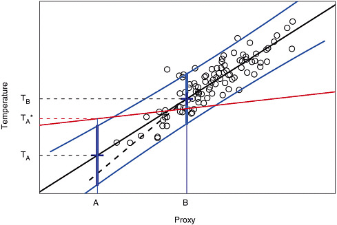
FIGURE 9-1 An illustration of using linear regression to predict temperature from proxy values. Plotted are 100 pairs of points corresponding to a hypothetical dataset of proxy observations and temperature measurements. The solid black line is the least-squares fitted line and the blue lines indicate 95 percent prediction intervals for temperature using this linear relationship. The dashed line and the red line indicate possible departures from a linear relationship between the proxy data and the temperature data. The figure also illustrates predictions made at proxy values A and B and the corresponding prediction intervals (wide blue lines) for the temperature.
values that are outside the range of proxy data used to estimate the linear relationship. In the case of multiple proxies used to predict temperature, it is not possible to use a two-dimensional graph to illustrate the fitted statistical model and the uncertainties. However, as in the single-proxy case, the prediction errors using several proxies will increase as the values deviate from those observed in the calibration period.
Variability in the Regression Predictions
Strictly speaking, assumption 1 posits a straight-line relationship between the average value of the climate variable, given the proxy, and the value of the proxy. This detail has the practical significance of potentially reducing the variability in the reconstructed series, which can also be illustrated using Figure 9-1. For example, note that there is some variability in the instrumental temperature measurements at the proxy value B (i.e., near point B, there are multiple temperature readings, most of which do not fall on the calibration line). However, estimates of past temperatures using proxy data near B will always yield the same temperature, namely TB, rather than a corresponding scatter of temperatures. This difference is entirely appropriate because TB is the most likely temperature value for each proxy measurement that yields B. In general, the predictions from regression will have less variability than the actual values, so time series of reconstructed temperatures will not fully reproduce the variability observed in the instrumental record.
One way to assess methods of reconstructing temperatures is to apply them to a synthetic history in which all temperatures are known. Zorita and von Storch (2005) and von Storch et al. (2004) carried out such an exercise using temperature output from the ECHO-G climate model. These authors constructed pseudoproxies by sampling the temperature field at locations used by Mann et al. (1998) and corrupted them with increasing levels of white noise. They then reconstructed the Northern Hemisphere average temperature using both regression methods and the related Mann et al. method and found that in both cases the variance of the reconstruction was attenuated relative to the “true” temperature time series with the attenuation increasing as the noise variance was increased.
This phenomenon, identified by Zorita and von Storch (2005) and others, is not unexpected. Within the calibration period, the fraction of variance of temperature that is explained by the proxies naturally decreases as the noise level of the proxies increases. If the regression equation is then used to reconstruct temperatures for another period during which the proxies are statistically similar to those in the calibration period, it would be expected to capture a similar fraction of the variance.
Some other approaches to reconstruction (e.g., Moberg et al. 2005b) yield a reconstructed series that has variability similar to the observed temperature series. These approaches include alternatives to ordinary regression methods such as inverse regression and total least-squares regression (Hegerl 2006) that are not subject to attenuation. Such methods may avoid the misleading impression that a graph of an attenuated temperature signal might give, but they do so at a price: Direct regression gives the most precise reconstruction, in the sense of mean squared error, so these other methods give up accuracy. Referring back to the example in Figure 9-1, using the straight-line relationship is the best prediction to make from these data, and any inflation of the variability will degrade the accuracy of the reconstruction.
Departures from the Assumptions
The dashed line in Figure 9-1 represents a hypothetical departure from the strict linear relationship between the proxy data and temperature. This illustrates a violation of the linearity assumption because, for lower values of the proxy, the relationship is not the same as given by the (straight) least-squares best-fit line. If the dashed line describes a more accurate representation of the relationship between the proxy values and temperature measurements at lower proxy values, then using the dashed line will result in different reconstructed temperature series.
The linear relationship among the temperature and proxy variables can also be influenced by whether the variables are detrended. If a temperature and a proxy time series share a common trend but are uncorrelated once the trends are removed, the regression analysis can give markedly different results. The regression performed without first removing a trend could exhibit a strong relationship, while the detrended regression could be weak. Whether to include a trend or not should be based on scientific understanding of the similarities or differences of the relationship over longer and shorter timescales.
A departure from the stationarity assumption is illustrated by the red line in Figure 9-1. Suppose that in a period other than the calibration period, the proxy and the temperature are related on average by the red line, that is, a different linear relationship from the one in the calibration period. For an accurate reconstruction, one would want to use this red line and the estimate for a temperature at the proxy value A is indicated by TA* in the figure.
Both the linearity and stationarity assumptions may be checked using the training and validation periods of the instrumental record. If the relationship is not linear over the training period, a variety of objective statistical approaches can be used to describe a more complicated relationship than a linear one. Moreover, one can contrast the effect of using detrended versus raw variables. Stationarity can also be tested for the validation period, although in most cases the use of the proxy relationship will involve extrapolation beyond the range of observed values, such as in the case of point A in the illustration given above. In cases such as this, the extrapolation must also rely on the scientific context for its validity; that is, one must provide a scientific basis for the assumed relationship.
The distinction between the assumptions used to reconstruct temperatures and the additional assumptions required to generate statistical measures of the uncertainty of such reconstructions is critical. For example, the error bounds in Figure 9-1 are based on statistical assumptions on how the temperature departs from an exact linear relationship. These assumptions can also be checked using the training and calibration periods, and often more complicated regression methods can be used to adjust for particular features in the data that violate the assumptions. One example is temporal correlation among data points, which is discussed in the next section.
Inverse Regression and Statistical Calibration
Reconstructing temperature or another climate variable from a proxy such as a tree ring parameter has a formal resemblance to the statistical calibration of a measurement instrument. A statistical calibration exercise consists of a sequence of experiments in which a single factor (e.g., the temperature) is set to precise, known levels,
and one or more measurements are made on a response (e.g., the proxy). Subsequently, in a second controlled experiment under identical conditions, the response is measured for an unknown level of the factor, and the regression relationship is used to infer the value of the factor. This approach is known as inverse regression (Eisenhart 1939) because the roles of the response and factor are reversed from the more direct prediction illustrated in Figure 9-1. Attaching an uncertainty to the result is nontrivial, but conservative approximations are known (Fieller 1954). There remains some debate in the statistical literature concerning the circumstances when inverse or direct methods are better (Osborne 1991).
The temperature reconstruction problem does not fit into this framework because both temperature and proxy values are not controlled. A more useful model is to consider the proxy and the target climate variable as a bivariate observation on a complex system. Now the statistical solution to the reconstruction problem is to state the conditional distribution of the unobserved part of the pair, temperature, given the value of the observed part, the proxy. This is also termed the random calibration problem by Brown (1982). If the bivariate distribution is Gaussian, then the conditional distribution is itself Gaussian, with a mean that is a linear function of the proxy and a constant variance. From a sample of completely observed pairs, the regression methods outlined above give unbiased estimates of the intercept and slope in that linear function. In reality, the bivariate distribution is not expected to follow the Gaussian exactly. In this case the linear function is only an approximation; however, the adequacy of these approximations can be checked based on the data using standard regression diagnostic methods. With multiple proxies, the dimension of the joint distribution increases, but the calculation of the conditional distribution is a direct generalization from the bivariate (single-proxy) case.
Regression with Correlated Data
In most cases, calibrations are based on proxy and temperature data that are sequential in time. However, geophysical data are often autocorrelated, which has the effect of reducing the effective sample size of the data. This reduction in sample size decreases the accuracy of the estimated regression coefficients and causes the standard error to be underestimated during the calibration period. To avoid these problems and form a credible measure of uncertainty, the autocorrelation of the input data must be taken into account.
The statistical strategy for accommodating correlation in the data used in a regression model is two-pronged. The first part is to specify a model for the correlation structure and to use modified regression estimates (generalized least squares) that achieve better precision. The correctness of the specification can be tested using, for example, the Durbin-Watson statistic (Durbin and Watson 1950, 1951, 1971). The second part of the strategy is to recognize that correlation structure is usually too complex to be captured with parsimonious models. This structure may be revealed by a significant Durbin-Watson statistic or some other test, or it may be suspected on other grounds. In this case, the model-based standard errors of estimated coefficients may be replaced by more robust versions, discussed for instance by Hinkley and Wang (1991). For time series data, Andrews (1991) describes estimates of standard errors that are consistent in the presence of autocorrelated errors with changing variances. For time series data, the correlations are usually modeled as stationary; parsimonious
models for stationary time series, such as ARMA, were popularized by Box and Jenkins (Box et al. 1994). Note that this approach does not require either the temperature or the proxy to be stationary, only the errors in the regression equation.
Reconstruction Uncertainty and Temporal Correlation
An indication of the uncertainty of a reconstruction is an important part of any display of the reconstruction itself. Usually this is in the form:
and the standard error is given by conventional regression calculations.
The prediction mean squared error is the square of the standard error and is the sum of two terms. One is the variance of the errors in the regression equation, which is estimated from calibration data, and may be modified in the light of differences between the calibration errors and the validation errors. This term is the same for all reconstruction dates. The other term is the variance of the estimation error in the regression parameters, and this varies in magnitude depending on the values of the proxies and also the degree of autocorrelation in the errors. This second term is usually small for a date when the proxies are well within the range represented by the calibration data, but may become large when the equation is used to extrapolate to proxy values outside that range.
Smoothed Reconstructions
Reconstructions are often shown in a smoothed form, both because the main features are brought out by smoothing and because the reconstruction of low-frequency features may be more precise than short-term behavior. The two parts of the prediction variance are both affected by smoothing but in different ways. The effect on the first depends on the correlation structure of the errors, which may require some further modeling, but is always a reduction in size. The second term depends on the smoothed values of the proxies and may become either larger or smaller but typically becomes a more important part of the resulting standard error, especially when extrapolating.
PRINCIPAL COMPONENT REGRESSION
The basic idea behind principal component regression is to replace the predictors (i.e., individual proxies) with a smaller number of objectively determined variables that are linear combinations of the original proxies. The new variables are designed to contain as much information as possible from the original proxies. As the number of principal components becomes large, the principal component regression becomes close to the regression on the full set of proxies. However, in practice the number of principal components is usually kept small, to avoid overfitting and the consequent loss of prediction skill. No known statistical theory suggests that limiting the number of principal components used in regression leads to good predictions, although this practice has been found to work well in many applications. Fritts et al. (1971) introduced the idea to dendroclimatology, and it was discussed by Briffa and Cook (1990).
Jolliffe (2002) describes many issues in the use of principal component analysis, including principal component regression, as it is used in many areas of science.
The principal components contain maximum information in the sense that the full set of proxies can be reproduced as closely as possible, given only the values of the new variables (Johnson and Wichern 2002, Suppl. 8A). In general, one should judge the set of principal components taken together as a group because they are used together to form a reconstruction. Comparing just single principal components between two different approaches may be misleading. For example, each of the two groups of principal components may give equally valid approximations to the full set of proxies. This equivalence can occur without being able to match on a one-to-one basis the principal components in one group with those in a second group.
Spurious Principal Components
McIntyre and McKitrick (2003) demonstrated that under some conditions the leading principal component can exhibit a spurious trendlike appearance, which could then lead to a spurious trend in the proxy-based reconstruction. To see how this can happen, suppose that instead of proxy climate data, one simply used a random sample of autocorrelated time series that did not contain a coherent signal. If these simulated proxies are standardized as anomalies with respect to a calibration period and used to form principal components, the first component tends to exhibit a trend, even though the proxies themselves have no common trend. Essentially, the first component tends to capture those proxies that, by chance, show different values between the calibration period and the remainder of the data. If this component is used by itself or in conjunction with a small number of unaffected components to perform reconstruction, the resulting temperature reconstruction may exhibit a trend, even though the individual proxies do not. Figure 9-2 shows the result of a simple simulation along the lines of McIntyre and McKitrick (2003) (the computer code appears in Appendix B). In each simulation, 50 autocorrelated time series of length 600 were constructed, with no coherent signal. Each was centered at the mean of its last 100 values, and the first principal component was found. The figure shows the first components from five such simulations overlaid. Principal components have an arbitrary sign, which was chosen here to make the last 100 values higher on average than the remainder.
Principal components of sample data reflect the shape of the corresponding eigenvectors of the population covariance matrix. The first eigenvector of the covariance matrix for this simulation is the red curve in Figure 9-2, showing the precise form of the spurious trend that the principal component would introduce into the fitted model in this case.
This exercise demonstrates that the baseline with respect to which anomalies are calculated can influence principal components in unanticipated ways. Huybers (2005), commenting on McIntyre and McKitrick (2005a), points out that normalization also affects results, a point that is reinforced by McIntyre and McKitrick (2005b) in their response to Huybers. Principal component calculations are often carried out on a correlation matrix obtained by normalizing each variable by its sample standard deviation. Variables in different physical units clearly require some kind of normalization to bring them to a common scale, but even variables that are physically equivalent or
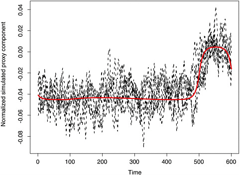
FIGURE 9-2 Five simulated principal components and the corresponding population eigenvector. See text for details.
normalized to a common scale may have widely different variances. Huybers comments on tree ring densities, which have much lower variances than widths, even after conversion to dimensionless “standardized” form. In this case, an argument can be made for using the variables without further normalization. However, the higher-variance variables tend to make correspondingly higher contributions to the principal components, so the decision whether to equalize variances or not should be based on the scientific considerations of the climate information represented in each of the proxies.
Each principal component is a weighted combination of the individual proxy series. When those series consist of a common signal plus incoherent noise, the best estimate of the common signal has weights proportional to the sensitivity of the proxy divided by its noise variance. These weights in general are not the same as the weights in the principal component, as calculated from either raw or standardized proxies, either of which is therefore suboptimal. In any case, the principal components should be constructed to achieve a low-dimensional representation of the entire set of proxy variables that incorporates most of the climate information contained therein.
VALIDATION AND THE PREDICTION SKILL OF THE PROXY RECONSTRUCTION
The role of a validation period is to provide an independent assessment of the accuracy of the reconstruction method. As discussed above, it is possible to overfit the statistical model during the calibration period, which has the effect of underestimating the prediction error. Reserving a subset of the data for validation is a natural way to offset this problem. If the validation period is independent of the calibration period, any skill measures used to assess the quality of the reconstruction will not be biased by the potential overfit during the calibration period. An inherent difficulty in validating a climate reconstruction is that the validation period is limited to the historical instrumental record, so it is not possible to obtain a direct estimate of the reconstruction skill at earlier periods. Because of the autocorrelation in most geophysical time series, a validation period adjacent to the calibration period cannot be truly independent; if the autocorrelation is short term, the lack of independence does not seriously bias the validation results.
Measures of Prediction Skill
Some common measures used to assess the accuracy of statistical predictions are the mean squared error (MSE), reduction of error (RE), coefficient of efficiency (CE), and the squared correlation (r2). The mathematical definitions of these quantities are given in Box 9.1. MSE is a measure of how close a set of predictions are to the actual values and is widely used throughout the geosciences and statistics. It is usually normalized and presented in the form of either the RE statistic (Fritts 1976) or the CE statistic (Cook et al. 1994). The RE statistic compares the MSE of the reconstruction to the MSE of a reconstruction that is constant in time with a value equivalent to the sample mean for the calibration data. If the reconstruction has any predictive value, one would expect it to do better than just the sample average over the calibration period; that is, one would expect RE to be greater than zero.
The CE, on the other hand, compares the MSE to the performance of a reconstruction that is constant in time with a value equivalent to the sample mean for the validation data. This second constant reconstruction depends on the validation data, which are withheld from the calibration process, and therefore presents a more demanding comparison. In fact, CE will always be less than RE, and the difference increases as the difference between the sample means for the validation and the calibration periods increases.
If the calibration has any predictive value, one would expect it to do better than just the sample average over the validation period and, for this reason, CE is a particularly useful measure. The squared correlation statistic, denoted as r2, is usually adopted as a measure of association between two variables. Specifically, r2 measures the strength of a linear relationship between two variables when the linear fit is determined by regression. For example, the correlation between the variables in Figure 9-1 is 0.88, which means that the regression line explains 100 × 0.882 = 77.4 percent of the variability in the temperature values. However, r2 measures how well some linear function of the predictions matches the data, not how well the predictions themselves perform. The coefficients in that linear function cannot be calculated without knowing the values being predicted, so it is not in itself a useful indication of merit. A high CE
|
BOX 9.1 Measures of Reconstruction Accuracy Let yt denote a temperature at time t and ŷt the prediction based on a proxy reconstruction. Mean squared error (MSE) where the sum on the right-hand side of the equation is over times of interest (either the calibration or validation period) and N is the number of time points. Reduction of error statistic (RE) where Coefficient of efficiency (CE) where Squared correlation (r2 ) If ŷt are the predictions from a linear regression of yt on the proxies, and the period of interest is the calibration period, then RE, CE, and r2 are all equal. Otherwise, CE is less than both RE and r2. |
value, however, will always have a high r2, and this is another justification for considering the CE.
Illustration of CE and r2
Figure 9-3 gives some examples of a hypothetical temperature series and several reconstruction series, where the black line is the actual temperatures and the colored lines are various reconstructions. The red line has an r2 of 1 but a CE of –18.9 and is
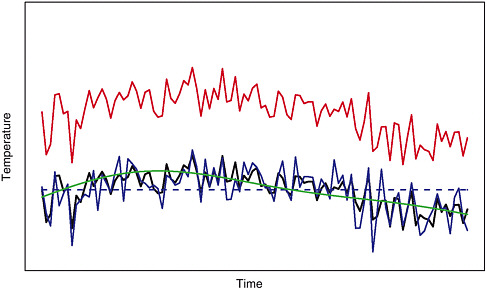
FIGURE 9-3 A hypothetical temperature series (black line) and four possible reconstructions.
an example of a perfectly correlated reconstruction with no skill at prediction. The dashed blue line is level at the mean temperature and has an r2 and a CE that are both zero. The blue and green reconstructed lines both have a CE of 0.50. For either of these reconstructions to be better than just the mean, they must exhibit some degree of correlation with the temperatures. In this case, r2 is 0.68 for the blue line and 0.51 for the green line.
Despite a common CE, these two reconstructions match the temperature series in different ways. The blue curve is more highly correlated with the short-term fluctuations, and the green curve tracks the longer term variations of the temperature series. The difference between the blue and green lines illustrates that the CE statistic alone does not contain all the useful information about the reconstruction error.
Distinguishing Between RE and CE and the Validation Period
The combination of a high RE and a low CE or r2 means that the reconstruction identified the change in mean levels between the calibration and validation periods reasonably well but failed to track the variations within the validation period. One way that this discrepancy can occur is for the proxies and the temperatures to be related by a common trend in the calibration period. When the trend is large this can result in a high RE. If the validation period does not have as strong a trend and the proxies are not skillful at predicting shorter timescale fluctuations in temperature, then the CE can be substantially lower. For example, the reconstructions may only do as
well as the mean level in the validation period, in which case CE will be close to zero. An ideal validation procedure would measure skill at different timescales, or in different frequency bands using wavelet or power spectrum calculations. Unfortunately, the paucity of validation data places severe limits on their sensitivity. For instance, a focus on variations of decadal or longer timescales with the 45 years of validation data used by Mann et al. (1998) would give statistics with just (2 × 45 ÷ 10) = 9 degrees of freedom, too few to adequately quantify skill. This discussion also motivates the choice of a validation period that exhibits the same kind of variability as the calibration period. Simply using the earliest part of the instrumental series may not be the best choice for validation.
Determining Uncertainty and Selecting Among Statistical Methods
Besides supplying an unbiased appraisal of the accuracy of the reconstruction, the validation period can also be used to adjust the uncertainty measures for the reconstruction. For example, the MSE calculated for the validation period provides a useful measure of the accuracy of the reconstruction; the square root of MSE can be used as an estimate of the reconstruction standard error. Reconstructions that have poor validation statistics (i.e., low CE) will have correspondingly wide uncertainty bounds, and so can be seen to be unreliable in an objective way. Moreover, a CE statistic close to zero or negative suggests that the reconstruction is no better than the mean, and so its skill for time averages shorter than the validation period will be low. Some recent results reported in Table 1S of Wahl and Ammann (in press) indicate that their reconstruction, which uses the same procedure and full set of proxies used by Mann et al. (1999), gives CE values ranging from 0.103 to –0.215, depending on how far back in time the reconstruction is carried. Although some debate has focused on when a validation statistic, such as CE or RE, is significant, a more meaningful approach may be to concentrate on the implied prediction intervals for a given reconstruction. Even a low CE value may still provide prediction intervals that are useful for drawing particular scientific conclusions.
The work of Bürger and Cubasch (2005) considers different variations on the reconstruction method to arrive at 64 different analyses. Although they do not report CE, examination of Figure 1 in their paper suggests that many of the variant reconstructions will have low CE and that selecting a reconstruction based on its CE value could be a useful way to winnow the choices for the reconstruction. Using CE to judge the merits of a reconstruction is known as cross-validation and is a common statistical technique for selecting among competing models and subsets of data. When the validation period is independent of the calibration period, cross-validation avoids many of the issues of overfitting if models were simply selected on the basis of RE.
QUANTIFYING THE FULL UNCERTAINTY OF A RECONSTRUCTION
The statistical framework based on regression provides a basis for attaching uncertainty estimates to the reconstructions. It should be emphasized, however, that this is only the statistical uncertainty and that other sources of error need to be addressed from a scientific perspective. These sources of error are specific to each proxy and are discussed in detail in Chapters 3–8 of this report. The quantification of statistical uncertainty depends on the stationarity and linearity assumptions cited above, the
adjustment for temporal correlation in the proxy calibration, and the sensible use of principal components or other methods for data reduction. On the basis of these assumptions and an approximate Gaussian distribution for the noise in the relationship between temperature and the proxies, one can derive prediction intervals for the reconstructed temperatures using standard techniques (see, e.g., Draper and Smith 1981). This calculation will also provide a theoretical MSE for the validation period, which can be compared to the actual mean squared validation error as a check on the method.
One useful adjustment is to inflate the estimated prediction standard error (but not the reconstruction itself) in the predictions so that they agree with the observed CE or other measures of skill during the validation period. This will account for the additional uncertainty in the predictions that cannot be deduced directly from the statistical model. Another adjustment is to use Monte Carlo simulation techniques to account for uncertainty in the choice of principal components. Often, 10-, 30-, or 50-year running means are applied to temperature reconstructions to estimate long-term temperature averages. A slightly more elaborate computation, but still a standard technique in regression analysis, would be to derive a covariance matrix of the uncertainties in the reconstructions over a sequence of years. This would make it possible to provide a statistically rigorous standard error when proxy-based reconstructions are smoothed.
Interpreting Confidence Intervals
A common way of reporting the uncertainty in a reconstruction is graphing the reconstructed temperature for a given year with the upper and lower limits of a 95 percent confidence interval to quantify the uncertainty. Usually, the reconstructed curve is plotted with the confidence intervals forming a band about the estimate. The fraction of variance that is not explained by the proxies is associated with the residuals, and their variance is one part of the mean squared prediction error, which determines the width of the error band.
Although this way of illustrating uncertainty ranges is correct, it can easily be misinterpreted. The confusion arises because the uncertainty for the reconstruction is shown as a curve, rather than as a collection of points. For example, the 95 percent confidence intervals, when combined over the time of the reconstruction, do not form an envelope that has 95 percent probability of containing the true temperature series. To form such an envelope, the intervals would have to be inflated further with a factor computed from a statistical model for the autocorrelation, typically using Monte Carlo techniques. Such inflated intervals would be a valid description of the uncertainty in the maximum or minimum of the reconstructed temperature series.
Other issues also arise in interpreting the shape of a temperature reconstruction curve. Most temperature reconstructions exhibit a characteristic variability over time. However, the characteristics of the unknown temperature series may be quite different from those of the reconstruction, which must always be borne in mind when interpreting a reconstruction. For example, one might observe some decadal variability in the reconstruction and attribute similar variability to the real temperature series. However, this inference is not justified without further statistical assumptions, such as the probability of a particular pattern appearing due to chance in a temporally correlated series. Given the attenuation in variability associated with the regression method and the temporal correlations within the proxy record that may not be related to tempera-
ture, quantifying how the shape of the reconstructed temperature curve is related to the actual temperature series is difficult.
Ensembles of Reconstructions
One approach to depicting the uncertainty in the reconstructed temperature series is already done informally by considering a sample, or ensemble, of possible reconstructions. By graphing different approaches or variants of a reconstruction on the same axes, such as Figure S-1 of this report, differences in variability and trends can be appreciated. The problem with this approach is that the collection of curves cannot be interpreted as a representative sample of some population of reconstructions. This is also true of the 64 variants in Bürger and Cubasch (2005). The differences in methodology and datasets supporting these reconstructions make them distinct, but whether they represent a deliberate sample from the range of possible temperature reconstructions is not clear. As an alternative, statistical methods exist for generating an ensemble of temperature reconstructions that can be interpreted in the more traditional way as a random sample. Although this requires additional statistical assumptions on the joint distribution of the proxies and temperatures, it simplifies the interpretation of the reconstruction. For example, to draw inferences about the maximum values in past temperatures, one would just form a histogram of the maxima in the different ensemble members. The spread in the histogram is a rigorous way to quantify the uncertainty in the maximum of a temperature reconstruction.


