Human Biomonitoring for Environmental Chemicals (2006)

Chapter 5 describes a variety of approaches for interpreting biomonitoring results, ranging from direct application of biomarker-response relationships found in epidemiologic studies to physiologically based pharmokinetic (PBPK) modeling based on animal data. Although Chapter 5 provides several chemical examples of the approaches described, the additional case studies discussed in this appendix are useful to illustrate the data needs and limitations.

Chapter 5 described general limitations of extrapolating workplace biomarker indices, such as Biological Exposure Indices (BEIs) to the general public. However, biomarker-exposure dose relationships established in the workplace may have utility for developing pharmacokinetic models that could be used to interpret biomonitoring data on the general public.

The chlorpyrifos and phthalate examples demonstrate that urinary biomarker data can be used within the context of pharmacokinetic modeling to interpret human exposure and risk. For a number of workplace urinary biomarkers, simple approaches have been used to relate biomarker concentration to exposure dose. A prime example is styrene: an empirically derived relationship between urinary concentration of the metabolite, man-

delic acid, and the workplace air concentration has been developed (ACGIH 1991). A commonly used BEI for styrene is based on that urinary measure. Different equations are available to convert urinary concentration from milligrams per liter of urine or from milligrams per gram of creatinine back to a time-weighted average inhaled concentration. The urinary biomarker has been used to test correlations between styrene exposure and adverse effects in worker populations with respect to sperm DNA abnormalities, neurologic effects, and renal effects (Lindstrom et al. 1976a,b; Harkonen 1977; Vyskocil et al. 1989; Migliore et al. 2002).

The empirical relationship between urinary biomarker and ambient concentration has utility for screening worker populations, but less utility for risk assessment in the general population. The equations are valid only if urine is collected after an 8-hour workshift. Furthermore, the relationship between amount in urine and air concentration will depend on level of exertion and respiratory rate, which may differ between the workplace and the general population. Those limitations will generally occur with any occupation-based algorithm for relating urinary biomonitoring results to air concentration or exposure dose. However, such empirical data can be used to calibrate pharmacokinetic models that can take into account exposure and physiologic variables and thus can be applicable to both the workplace and the general population. The example described elsewhere for the chlorpyrifos metabolite is a case in point.

Regarding styrene, the variety of controlled human oral and inhalation studies that relate dose to urinary concentration and the existence of a pharmacokinetic model (Droz and Guillemin 1983) could facilitate interpretation of mandelic acid concentration in urine. A caveat in this regard is that other chemical exposures can produce mandelic acid in urine, such as ethyl benzene, acetophenone, and phenylglycine (ACGIH 1991). Those “background” sources would be more likely to confound low-level general-population biomarker results than workplace end-of-shift results.

It is noteworthy that the styrene reference concentration (RfC) in the Integrated Risk Information System is based on the biomarker-response relationship found in workers (Mutti et al. 1984; EPA 1998). The Environmental Protection Agency (EPA) used the relationship of urinary biomarker to ambient-air concentration of workers to develop an RfC that was adjusted for the difference in exposure time between the workplace and the general population. That is a valid approach because it derives a workplace concentration-toxicity relationship in workers, which can then be adjusted for the general population to account for differences in exposure time and can take uncertainty factors into account. It is different from direct adjustment of the styrene BEI to evaluate human population biomonitoring data on styrene metabolites in urine, which would have the uncertainties described above and in Chapter 5.

In addition to the lead example presented in Chapter 5, the work done with methylmercury is an important illustration of the great utility of biomarker-effects data from human studies. The EPA’s risk assessment of methylmercury is based on such data generated in prospective epidemiologic research on effects of in utero exposure and adverse postnatal neuropsychologic sequelae (NRC 2000; Rice et al. 2003). Two biomarkers were used in the risk assessment: mercury in maternal hair collected at delivery and mercury in umbilical cord blood. Both biomarkers appear to be reliable internal dosimeters for exposure to methylmercury during pregnancy. The mercury biomarker in hair and blood is total mercury, including inorganic and organic forms. For the most part, that biomarker represents methylmercury from fish consumption in that this is the major source of systemically absorbed mercury. Total mercury in hair constitutes a relevant dosimeter in that it indicates the amount of methylmercury entering the hair follicle from the bloodstream and thus reflects the systemic concentration (Myers et al. 2003).¹ Umbilical-cord blood concentration would be expected to correlate most closely with fetal-brain concentration during late gestation (NRC 2000).

Two of the epidemiologic studies used in EPA’s risk assessment—those conducted in the Faroe Islands and New Zealand (Kjellström et al. 1986; Kjellstrom et al. 1989; Grandjean et al. 1997)—documented a significant inverse biomarker-neurodevelopment relationship.² Effects included poor performance on a number of tests—tests of attention, fine-motor function, language, visual-spatial abilities, and verbal memory. The magnitude of the deficits was consistent with increases in the number of children struggling to keep up in school or requiring remedial action (Rice et al. 2003). Those effects correlated with hair mercury in both studies; cord blood showed the

strongest association with the effects in the study where it was analyzed (Grandjean et al. 1997). The National Research Council (2000) analysis of the epidemiologic studies selected the Faroe Islands study as the lead dataset for dose-response modeling (NRC 2000). After that, EPA conducted a benchmark dose analysis of the cord blood-neurotoxicity relationship stemming from the Faroe Islands dataset (Rice et al. 2003); it yielded a biomarker benchmark dose of 58 µg/L (a cord-blood concentration of 58 µg/L is the 95% lower confidence limit of the dose associated with a 5% increase in neurodevelopmental effects). EPA used a one-compartment model to extrapolate from cord-blood mercury to the corresponding methylmercury intake by the mother. An uncertainty factor of 10 was incorporated into the risk assessment to account for intraindividual variability. The resulting reference-dose (RfD) calculations yielded 0.1 mg/kg per day (Rice et al. 2003).

Recent biomonitoring data from the 1999-2000 National Health and Nutrition Examination Surveys (NHANES) have been used to estimate the proportion of newborn infants in the United States that have been exposed to mercury in utero at above the EPA RfD (Mahaffey et al. 2004). The consumption of methylmercury from fish and other seafood constitutes the main source of dietary mercury exposure in the general population (CDC 2005). Analyses indicate that U.S. women of reproductive age generally have blood mercury below 58 µg/L. However, an estimated 5.7% have blood mercury between 5.8 µg/L and 58 µg/L (CDC 2005; Mahaffey et al. 2004). It has been estimated that in the United States more than 300,000 newborns each year are exposed to methylmercury in utero at concentrations above the RfD (Mahaffey et al., 2004) and within 10-fold of the concentrations associated with a 5% increase above background in neurodeveopmental effects. There has been controversy regarding the extent to which exposures above the RfD, but below 58 µg/L, translate into risk. However, an analysis estimated that 8,000 children are born each year in the United States with cord mercury levels 3.8 times the RfD or at exposure levels similar to those among women in the Faroe Islands (Clewell and Crump 2005). Exposures at this level were estimated to correspond to changes in the mean test score of 1.6% for neuropsychological function that were used in the Faroe Island research (the Boston naming test) (Clewell and Crump 2005). In addition, blood mercury in excess of 58 µg/L has been documented among some groups that consume much fish, including anglers, subsistence fisherman, and members of some American Indian tribes (Mahaffey et al. 2004).

This illustration shows how biomarker-based risk posed by methylmercury (5.8 µg/L as a blood equivalent of the RfD and 58 µg/L as a minimal effect concentration in human fish-eating populations, according to benchmark dose analysis) can be used directly to interpret population biomonitoring data. Pathway analyses conducted by others (Stern et al. 2001; Carrington

and Bolger 2002) have shown that some species of fish may be the most important source of methyl-mercury exposure; this presents a potential for intervention and future lowering of biomonitored concentrations.

As described in Chapter 5, one source of information that may assist in the interpretation of biomonitoring data is a pre-existing risk assessment. An example is glyphosate, a commonly used herbicide for which a traditional risk assessment is available from EPA as part of its reregistration evaluation (62 Fed. Reg. 17723 [1997]). The risk assessment estimates general population dietary exposures to be 0.001-0.01 of the acute and chronic RfDs, even if infants and occupationally exposed groups are considered. General-population biomonitoring data on glyphosate are not available, but the urinary biomarker data available on farmers and their families (Acquavella et al. 2004) can be interpreted in light of EPA risk projections.

Another example is permethrin, an insecticide widely used on food crops and in residential and occupational settings (ATSDR 2003). A comprehensive exposure and risk assessment for permethrin by EPA analyzed a number of scenarios for the general population and for homeowner and professional spray appliers (70 Fed. Reg. 51790 [2005]). The analysis of general population exposure via food and drinking water did not find a substantial health risk. However, the residential and worker pesticide spray scenarios were associated with greater risks. Biomonitoring results for the permethrin metabolites urinary cis- and trans-3-3(2,2,-dichlorovinyl)-2,2-dimethylcyclopropane carboxylic acid show a highly skewed distribution with the majority of the population having no detectable metabolites and the upper 95th percentile having biomarker concentrations that are many times above the limit of detection (CDC 2005). The NHANES study design was intended to be representative of the general population, so one can tentatively evaluate the median biomarker results for permethrin in light of EPA’s general population risk assessment. Furthermore, the upper tail of the distribution may be considered in light of EPA’s pesticide application scenarios. An improved biomonitoring study design in which information is gathered on personal pesticide use would help to clarify the exposure assignments. The EPA assessment also shows that the highest potential risks are for toddlers from carpet contact after pesticide application. That shows that a potentially important subgroup was not part of the NHANES biomonitoring dataset in that children under 6 years old were not monitored.

There are numerous caveats in the use of pre-existing risk assessments to interpret biomonitoring datasets, especially if it is not possible to relate the biomonitoring result to the exposure dose and if the population that the

risk assessment was based on differs in some way from the biomonitored population. Other caveats apply case by case. For the permethrin example, the biomonitoring data present issues of biomarker nonspecificity (cypermethrin and cyfluthrin also generate the urinary biomarkers, and a mix of permethrin biomarkers may be most informative), and there are detection-limit issues, as evidenced by the preponderance of nondetection results. The permethrin risk assessment also carries the uncertainty that the potential for developmental toxicity after chronic exposures has not been adequately tested (Shafer et al. 2005).

Chapter 5 describes a simple one-compartment modeling approach that can yield screening-level estimates of intake dose based on biomonitoring results (chemical concentration in blood or lipid) for slowly cleared lipid-soluble chemicals. The overall approach is shown below (Figure B-1 is reproduced from Chapter 5):

A basic lipid-partitioning approach similar to that outlined above has been used for TCDD (van der Molen et al. 1996; Lorber and Phillips 2002; EPA 2003), organochlorine pesticides (LaKind et al. 2000; Lindstrom et al. 1976a), and polychlorinated biphenyls (PCBs) (Lutz et al. 1984). For application to interpreting biomonitoring results, the first step is conversion of the blood concentration to total body burden of chemical. For highly lipid-soluble chemicals that do not appreciably bind to proteins, that involves scaling up from the blood concentration with calculations that first express the concentration in blood on a lipid basis (TCDD concentration in blood lipid). The next step is to convert the lipid concentration to a total body burden by multiplying the blood concentration (lipid basis) by the total amount of lipid in the body. That assumes that the chemical will have the

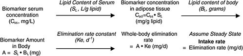
FIGURE B-1 Conversion of biomonitoring data to daily dose on the basis of one-compartment (body-burden) model.

same concentration in all lipid compartments of the body. The resulting body burden undergoes a daily loss at a rate based on its elimination via renal or, in the case of TCDD, hepatic (metabolic) clearance. The long-term rate of elimination from blood is used because it represents true clearance from the body without the influence of continuing absorption or chemical redistribution. Although such half-life information has been estimated in humans for organochlorines, it is not quite accurate, because there is typically low-level exposure after earlier periods of higher (for example, occupational) exposure. Nevertheless, such total-body clearance rates can provide a useful estimate for calculating the daily clearance rate, which, under the assumption of steady state (no change in body burden), must be balanced by chemical intake.

The one-compartment approach has been used to estimate background exposure to TCDD in the general population on the basis of serum or adipose measurements with the following equation (EPA 2003):

where dose is in picograms per day, half-life (t_1/2) is in years, volume body fat is in kilograms, concentration in body fat is in picograms per kilogram, CF₁ is a conversion factor in grams per kilogram, and CF₂ is a conversion factor in years per day.

For TCDD and related congeners, a traditional pathway analysis has also been conducted. The daily dose estimated from extrapolation of biomonitoring results is in a similar range as the estimates from exposure-pathway calculations (EPA 2003). That suggests that the conversion of biomonitoring results to an exposure dose may be feasible when pharmacokinetic information (chemical half-life in humans) is relatively sparse. However, this applies only to steady-state conditions in which the biomonitoring result reflects a stable level from long-term storage in lipid with slow elimination. Under those conditions, it is fairly straightforward to calculate body burden and thus convert the long-term half-life to a total-body loss rate that one assumes (at steady state) is matched by the intake rate. That approach may be applicable to PCBs and other persistent organochlorines, but it is less feasible for other types of chemicals.

A caveat with this approach is the potential for variability in elimination rate. The biologic half-life of TCDD has been estimated at 3-27 years in people chronically exposed to TCDD; central-tendency half-lives are reported as 5.8-8.7 years in various studies (Pirkle et al. 1989; Michalek et al. 1996; Ott and Zober 1996). At least some of the variability is due to different sizes of the body lipid compartment and to variable activity of the CYP1A family to metabolize TCDD (EPA 2003). In fact, there is some

support for the idea that the higher the TCDD body burden, the shorter the half-life, because TCDD induces the CYP1A family of enzymes through which it is metabolized (Carrier et al. 1995). There is also greater binding to hepatic proteins when metabolizing systems are induced by TCDD, and this alters chemical distribution (Abraham et al. 1988). A recent PBPK modeling approach for dioxin takes into account inducible elimination (Emond et al. 2005a); PBPK modeling of PCBs was recently used to simulate changing blood concentrations over short periods (Emond et al. 2005b).

Chlorpyrifos provides an example of the utility of human pharmacokinetic models to estimate daily dose from biomonitoring data for a rapidly cleared pesticide. The urinary metabolite trichloro-2-pyridinol (TCP) is used in the NHANES study to monitor population exposure to chlorpyrifos (CDC 2005). Several epidemiologic studies have linked chlorpyrifos exposure to adverse birth outcomes through associations between urinary and blood biomarkers and have demonstrated maternal exposure and physiologic measurements in the neonate (Berkowitz et al. 2003, 2004; Whyatt et al. 2004; Needham 2005).

However, chlorpyrifos exposures among the populations evaluated in these studies may have been higher than in the general population. Recent NHANES data suggest that regulatory limits on chlorpyrifos use in residential settings have succeeded in decreasing general population exposures compared with 1988-1994 (Barr et al. 2005; CDC 2005).

Further interpretation of urinary biomonitoring data has been attempted with pharmacokinetic simulations by using a relatively simple one-compartment model to convert urinary concentrations to intake doses (Rigas et al. 2001; Shurdut et al. 1998; Barr 2005). The key assumption needed for back-calculation of intake dose from urinary concentration is that 70% of the dose is excreted in the urine as TCP over a relatively short period.

Pharmacokinetic calculations yielded estimates of chlorpyrifos intake of 0.05-1 µg/kg per day in the general population. The model estimates compare favorably with pathway analysis estimates of aggregate chlorpyrifos exposure from numerous dose routes, including indoor inhalation, dermal contact, and food ingestion (Shurdut et al. 1998; Pang et al. 2002). The calculated exposure doses ranged from 0.02 to 1 µg/kg per day. Further

refinements in both the pharmacokinetic modeling and exposure pathway analyses may help to narrow the range of estimated doses.

A more detailed seven-compartment human PBPK model for chlorpyrifos was calibrated against pharmacokinetic data in human subjects (Timchalk et al. 2002). The model can predict urinary output of TCP for a wide range of chlorpyrifos doses and exposure scenarios and so may be useful in refining the interpretation of population biomonitoring. That may be particularly important because the degree to which population biomonitoring results reflect steady-state conditions is not known and, for a rapidly eliminated biomarker, requires fairly constant exposure. More advanced modeling approaches can derive the biomonitoring serum concentration with a variety of different exposure scenarios (such as isolated bolus exposures vs low-level continuous exposures) in a sensitivity analysis to explore the risk implications of particular biomonitoring results (Rigas et al. 2001).

An important caveat in interpreting chlorpyrifos metabolite concentrations in urine is that this metabolite (TCP) is widespread in the environment and thus can appear in urine as a result of direct intake as well as from conversion from a parent chemical (Lu et al. 2005; Wilson et al. 2003). For example, the concentration of TCP in foods can be greater than that of chlorypyrifos, and concentrations in house dust can be generally comparable (Morgan et al. 2005). Direct intake of TCP from environmental media makes extrapolation of urinary biomarker concentration to chlorpyrifos exposure dose uncertain.

Solvents are typically not targeted for biomonitoring in general population studies, because their rapid clearance by exhalation or metabolism results in a transient biomarker that does not reach steady state. However, analysis of such rapidly cleared chemicals may be possible, as exemplified in a trichloroethylene (TCE) biomarker study (Sohn et al. 2004), which constitutes another case study of pharmacokinetic modeling of human biomonitoring data under non-steady-state conditions.

The biomonitoring data are based on a study of eight subjects exposed in a chamber for 4 hours to TCE at 100 ppm (Fisher et al. 1998). TCE blood concentrations were followed during exposure and for 12 hours afterward to demonstrate the buildup of TCE and its clearance from blood in each subject. (TCE is eliminated from blood rapidly, with a half-life of minutes to hours.)

A PBPK model was used to simulate the data but was then analyzed in reverse, starting with blood concentrations but missing the exposure infor-

mation (TCE concentration, sampling time, and exposure duration). The goal was to determine whether a Bayesian inference approach could be used to predict the exposure conditions for the eight subjects on the basis of their biomarker data and the PBPK model. Initial predictions of TCE blood concentrations were based on a set of “priors,” or modeling starting points. Monte Carlo analysis was used to present a full spectrum of TCE blood concentrations by using distributions rather than point estimates for a variety of PBPK modeling inputs. Because the “prior” information did not include exposure information, the initial TCE blood estimates were highly variable and not very precise. The updated, or “posterior,” estimates were based on a backfit that minimized the error between the model-predicted and actual biomonitoring data. The reconstructed exposure profiles yielded estimates of TCE concentration in air and other exposure characteristics (onset and duration) that were reasonably close to the actual experiment, although there was still a large degree of uncertainty in the estimates. The uncertainty could probably be reduced by improved information on behaviors that lead to exposure; for example, if onset and duration were more certain, TCE air concentration estimates would be improved.

Fisher 1998 demonstrates that the more that is learned about the biomarker (half-life, time course in blood or urine, and development of PBPK model) and the exposed population (age, body weight, pharmacoge-netic traits, behavioral factors that affect exposure, and time between exposure and sample measurement), the more refined dose estimates can become. Without such information, a highly transient metabolite like TCE is not a reliable marker of exposure, unless exposure is nearly continuous and uniform. That may not be the case in the general population, so TCE in blood may not be a good biomarker for assessment of general-population exposure, although PBPK models are available to extrapolate from biomarker concentration to external dose in both animals and humans (Clewell et al. 2000).

PBPK and Bayesian inference approaches analyze multiple sources of uncertainty and variability and thus have the potential to improve estimates of exposure (for example, time-weighted average air concentration) from TCE concentrations in blood. However, those techniques are data-intensive and time-consuming (although no more demanding than other methods of back-estimation). A simpler bounding approach may be useful as a first step in trying to reconstruct an exposure dose from biomonitoring data on short-lived biomarkers. Figure B-2 shows a simulated blood-concentration curve for a volatile organic chemical like TCE after a bolus exposure. A particular biomonitoring blood concentration can come from any point along the time course because it is not known when the sample was taken relative to the exposure events (sampling-time variability). If one assumes that the sample came from the left end of the curve (Figure B-2), reflecting

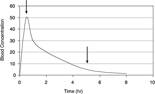
FIGURE B-2 Time course for VOC concentrations in blood after a bolus dose. Arrows indicate two of the many time points when a biomonitoring sample may be taken. Without prior knowledge, a useful screening approach is to assume that the sample was taken at the 5-hour arrow, well after the peak blood concentration. If that assumption is used across the population, a pharmacokinetic model can yield reasonably conservative bounding estimates of exposure dose. (Many exposure events might occur in a single day that could affect the concentration-time course of the VOCs in blood.)

peak internal exposure (first arrow), the PBPK model will predict a relatively low exposure concentration. If one assumes that the sample came from a late time when most TCE is washed out of the blood (second arrow), the model will convert this biomonitored concentration to a high exposure dose.

Thus, for screening purposes, one can project high-end exposure doses for rapidly cleared biomarkers by running the human PBPK model with the assumption that the sample was taken after multiple half-lives had elapsed from the exposure event. The high-end exposure estimates could be used in an initial risk assessment to compare with the RfD or other toxicity benchmarks. If the risk estimate is below a level of concern, there may not be a need for a more refined analysis. However, if it is high, it will trigger a more complete analysis in which the entire pharmacokinetic profile will be used in a probabilistic (Monte Carlo) setting that involves inference techniques. A high degree of variability in the biomonitoring data or many overlapping exposure episodes in a single person would make these approaches more complex but still valuable. The more information on the exposure and

sampling events (for example, samples collected in a clinic away from the home environment and thus several hours away from exposure sources), the more refined the dose prediction.

Abraham, K., R. Krowke, and D. Neubert. 1988. Pharmacokinetics and biological activity of 2,3,7,8-tetrachlorodibenzo-p-dioxin. 1. Dose-dependent tissue distribution and induction of hepatic ethoxyresorufin O-deethylase in rats following a single injection. Arch. Toxicol. 62(5):359-368.

ACGIH (American Conference of Governmental Industrial Hygienists). 1991. Documentation of the Threshold Limit Values and Biological Exposure Indices, 6th Ed. American Conference of Governmental Industrial Hygienists, Cincinnati, OH.

Acquavella, J.F., B.H. Alexander, J.S. Mandel, C. Gustin, B. Baker, P. Chapman, and M. Bleeke. 2004. Glyphosate biomonitoring for farmers and their families: Results from the Farm Family Exposure Study. Environ. Health Perspect. 112(3):321-326.

ATSDR (Agency for Toxic Substances and Disease Registry). 2003. Toxicological Profile for Pyrethrins and Pyrethroids. U.S. Department of Health and Human Service, Public Health Service, Agency for Toxic Substances and Disease Registry Service [online]. Available:http://www.atsdr.cdc.gov/toxprofiles/tp155.html [accessed Jan. 19, 2006].

Barr, D.B., R. Allen, A.O. Olsson, R. Bravo, L.M. Caltabiano, A. Montesano, J. Nguyen, S. Udunka, D. Walden, R.D. Walker, G. Weerasekera, R.D. Whitehead Jr, S.E. Schober, and L.L. Needham. 2005. Concentrations of selective metabolites of organophosphorus pesticides in the United States population. Environ. Res. 99(3):314-326.

Berkowitz, G.S., J. Obel, E. Deych, R. Lapinski, J. Godbold, Z. Liu, P.J. Landrigan, and M.S. Wolff. 2003. Exposure to indoor pesticides during pregnancy in a multiethnic, urban cohort. Environ. Health Perspect. 111(1):79-84.

Berkowitz, G.S., J.G. Wetmur, E. Birman-Deych, J. Obel, R.H. Lapinski, J.H. Godbold, I.R. Holzman, and M.S. Wolff. 2004. In utero pesticide exposure, maternal paraoxonase activity, and head circumference. Environ. Health Perspect. 112(3):388-391.

Carrier, G., R.C. Brunet, and J. Brodeur. 1995. Modeling of the toxicokinetics of polychlorinated dibenzo-p-dioxins and dibenzofurans in mammalians, including humans. I. Nonlinear distribution of PCDD/PCDF body burden between liver and adipose tissues. Toxicol. Appl. Pharmacol. 131(2):253-266.

Carrington, C.D., and M.P. Bolger. 2002. An exposure assessment for methylmercury from seafood for consumers in the United States. Risk Anal. 22(4):689-99.

CDC (Centers for Disease Control and Prevention). 2005. Third National Report on Human Exposure to Environmental Chemicals. U.S. Department of Health and Human Services, Centers for Disease Control and Prevention, Atlanta, GA [online]. Available: http://www.cdc.gov/exposurereport/3rd/ [accessed Nov. 16, 2005].

Clewell, H.J., and K.S. Crump. 2005. Quantitative estimates of risk for noncancer endpoints. Risk Anal. 25(2):285-289.

Clewell, H.J., P.R. Gentry, T.R. Covington, and J.M. Gearhart. 2000. Development of a physiologically based pharmacokinetic model of trichloroethylene and its metabolites for use in risk assessment. Environ. Health Perspect. 108(Suppl. 2):283-306.

Droz, P.O., and M.P. Guillemin. 1983. Human styrene exposure. V. Development of a model for biological modeling. Int. Arch. Occup. Environ. Health 53(1):19-36.

Emond, E., M. Charbonneau, and K. Krishnan. 2005a. Physiologically based modeling of the accumulation in plasma and tissue lipids of a mixture of PCB congeners in female Sprague-Dawley rats. J. Toxicol. Environ. Health A 68(16):1393-1412.

Emond, C, J.E. Michalek, L.S. Birnbaum, and M.J. DeVito. 2005b. Comparison of the use of a physiologically based pharmacokinetic model and a classical pharmacokinetic model for dioxin exposure assessment. Environ. Health Perspect. 113(12):1666-1668.

EPA (U.S. Environmental Protection Agency). 1998. Styrene (CASRN 100-42-5). Integrated Risk Information System, U.S. Environmental Protection Agency [online]. Available: http://www.epa.gov/iris/subst/0104.htm [accessed Jan. 17, 2006].

EPA (U.S. Environmental Protection Agency). 2003. Exposure and Human Health Reassessment of 2,3,7,8-Tetrachlorodibenzo-p-Dioxin (TCDD) and Related Compounds National Academy Sciences (NAS) Review Draft, Oct, 2004 [online]. Available: http://www.epa.gov/ncea/pdfs/dioxin/nas-review/ [accessed Jan. 20, 2006].

Fisher, J.W., D. Mahle, and R. Abbas. 1998. A human physiologically based pharmacokinetic model for trichloroethylene and its metabolites, trichloroacetic acid and free trichloroethanol. Toxicol Appl Pharmacol. 152(2):339-359.

Grandjean, P., P. Weihe, R.F. White, F. Debes, S. Araki, K. Yokoyama, K. Murata, N. Sorensen, R. Dahl, and P.J. Jorgensen. 1997. Cognitive deficit in 7-year-old children with prenatal exposure to methylmercury. Neurotoxicol. Teratol. 19(6):417-428.

Harkonen, H. 1977. Relationship of symptoms to occupational styrene exposure and to the findings of electroencephalographic and psychological examinations. Int. Arch. Occup. Environ. Health 40(4):231-239.

Kjellström, T., P. Kennedy, S. Wallis, and C. Mantell. 1986. Physical and Mental Development of Children with Prenatal Exposure to Mercury from Fish. Stage 1: Preliminary Test at Age 4. Report 3080. Solna, Sweden: National Swedish Environmental Protection Board.

Kjellström, T., P. Kennedy, S. Wallis, A. Stewart, L. Friberg, B. Lind, T. Wutherspoon, and C. Mantell. 1989. Physical and Mental Development of Children with Prenatal Exposure to Mercury from Fish. Stage 2: Interviews and Psychological Tests at Age 6. Report 3642. Solna, Sweden: National Swedish Environmental Protection Board.

LaKind, J.S., C.M. Berlin, C.N. Park, D.Q. Naiman, and N.J. Gudka. 2000. Methodology for characterizing distributions of incremental body burdens of 2,3,7,8-TCDD and DDE from breast milk in North American nursing infants. J. Toxicol. Environ. Health A 59(8):605-639.

Lindstrom, F.T., J.W. Gillett, and S.E. Rodecap. 1976a. Distribution of HEOD (dieldrin) in mammals: III. Transport-transfer. Arch. Environ. Contam. Toxicol. 4(3):257-288.

Lindstrom, K., H. Harkonen, and S. Hernberg. 1976b. Disturbances in psychological functions of workers occupationally exposed to styrene. Scand. J. Work Environ. Health 2(3):129-139.

Lorber, M., and L. Phillips. 2002. Infant exposure to dioxin-like compounds in breast milk. Environ. Health Perspect. 110(6):A325-A332.

Lu, C., R. Bravo, L.M. Caltabiano, R.M. Irish, G. Weerasekera, and D.B. Barr. 2005. The presence of dialkylphosphates in fresh fruit juices: Implications for organophosphate pesticide exposure and risk assessment. J. Toxicol. Environ. Health 68(3):209-227.

Lutz, R.J., R.L. Dedrick, D. Tuey, I.G. Sipes, M.W. Anderson, and H.B. Matthews. 1984. Comparison of the pharmacokinetics of several polychlorinated biphenyls in mouse, rat, dog, and monkey by means of a physiological pharmacokinetic model. Drug Metab. Dispos. 12(5):527-535.

Mahaffey, K.R., R.P. Clickner, and C.C. Bodurow. 2004. Blood organic mercury and dietary mercury intake: National Health and Nutrition Examination Survey, 1999 and 2000. Environ. Health Perspect. 112(5):562-570.

Michalek, J.E., J.L. Pirkle, S.P. Caudill, R.C. Tripathi, D.G. Patterson Jr., and L.L. Needham. 1996. Pharmacokinetics of TCDD in veterans of Operation Ranch Hand: 10-year followup. J. Toxicol. Environ. Health 47(3):209-220.

Migliore, L., A. Naccarati, A. Zanello, R. Scarpato, L. Bramanti, and M. Mariani. 2002. Assessment of sperm DNA integrity in workers exposed to styrene. Hum. Reprod. 17(11):2912-2918.

Morgan, M.K., L.S. Sheldon, C.W. Croghan, P.A. Jones, G.L. Robertson, J.C. Chuang, N.K. Wilson, and C.W. Lyu. 2005. Exposures of preschool children to chlorpyrifos and its degradation product 3,5,6-trichloro-2-pyridinol in their everyday environments. J. Expo. Anal. Environ. Epidemiol. 15(4):297-309.

Mutti, A., A. Mazzucchi, P. Rustichelli, G. Frigeri, G. Arfini, and I. Franchini. 1984. Exposure-effect and exposure-response relationships between occupational exposure to styrene and neuropsychological functions. Am. J. Ind. Med. 5(4):275-286.

Myers, G.J., P.W. Davidson, C. Cox, C.F. Shamlaye, D. Palumbo, E. Cernichiari, J. Sloane-Reeves, G.E. Wilding, J. Kost, L.S. Huang, and T.W. Clarkson. 2003. Prenatal methyl mercury exposure from ocean fish consumption in the Seychelle child development study. Lancet 361(9370):1686-1692.

Needham, L.L. 2005. Assessing exposure to organophosphorus pesticides by biomonitoring in epidemiologic studies of birth outcomes. Environ. Health Perspect. 113(4):494-498.

NRC (National Research Council). 2000. Toxicological Effects of Methylmercury. Washington, DC: National Academy Press.

Ott, M.G., and A. Zober. 1996. Cause specific mortality and cancer incidence among employees exposed to 2,3,7,8-TCDD after a 1953 reactor accident. Occup. Environ. Med. 53(9):606-612.

Pang, Y., D.L. Macintosh, D.E. Camann, and P.B. Ryan. 2002. Analysis of aggregate exposure to chlorpyrifos in the NHEXAS-Maryland investigation. Environ. Health Perspect. 110(3):235-240.

Pirkle, J.L., W.H. Wolfe, D.G. Patterson, L.L. Needham, J.E. Michalek, J.C., Miner, M.R. Peterson, and D.L. Phillips. 1989. Estimates of the half-life of 2,3,7,8-tetrachlorodibenzo-p-dioxin in Vietnam Veterans of Operation Ranch Hand. J. Toxicol. Environ. Health 27(2):165-171.

Rice, D.C., R. Schoeny, and K. Mahaffey. 2003. Methods and rationale for derivation of a reference dose for methylmercury by the U.S. EPA. Risk Anal. 23(1):107-115.

Rigas, M.L., M.S. Okino, and J.J. Quackenboss. 2001. Use of a pharmacokinetic model to assess chlorpyrifos exposure and dose in children, based on urinary biomarker measurements. Toxicol. Sci. 61(2):374-381.

Shafer, T.J., D.A. Meyer, and K.M. Crofton. 2005. Developmental neurotoxicity of pyrethroid insecticides: Critical review and future research needs. Environ. Health Perspect. 113(2):123-136.

Shurdut, B.A., L. Barraj, and M. Francis. 1998. Aggregate exposures under the Food Quality Protection Act: An approach using chlorpyrifos. Regul. Toxicol. Pharmacol. 28(2): 165-177.

Sohn, M.D., T.E. McKone, and J.N. Blancato. 2004. Reconstructing population exposures from dose biomarkers: Inhalation of trichloroethylene (TCE) as a case study. J. Expo. Anal. Environ. Epidemiol. 14(3):204-213.

Stern, A.H., M. Gochfeld, C. Weisel, and J. Burger. 2001. Mercury and methylmercury exposure in the New Jersey pregnant population. Arch Environ Health. 56(1):4-10.

Timchalk, C., R.J. Nolan, A.L. Mendrala, D.A. Dittenber, K.A. Brzak, and J.L. Mattsson. 2002. A physiologically based pharmacokinetic and pharmacodynamic (PBPK/PD) model for the organophosphate insecticide chlorpyrifos in rats and humans. Toxicol. Sci 66(1): 34-53.

van der Molen, G.W., S.A. Kooijman, and W. Slob. 1996. A generic toxicokinetic model for persistent lipophilic compounds in humans: An application to TCDD. Fundam. Appl. Toxicol. 31(1):83-94.

Vyskocil, A., S. Emminger, F. Malir, Z. Fiala, M. Tusl, E. Ettlerova, and A. Bernard. 1989. Lack of nephrotoxicity of styrene at current TLV level (50 ppm). Int. Arch. Occup. Environ. Health 61(6):409-411.

Whyatt, R.M., V. Rauh, D.B. Barr, D.E. Camann, H.F. Andrews, R. Garfinkel, L.A. Hoepner, D. Diaz, J. Dietrich, A. Reyes, D. Tang, P.L. Kinney, and F.P. Perera. 2004. Prenatal insecticide exposures and birth weight and length among an urban minority cohort. Environ. Health Perspect. 112(10):1125-1132.

Wilson, N.K., J.C. Chuang, C. Lyu, R. Menton, and M.K. Morgan. 2003. Aggregate exposures of nine preschool children to persistent organic pollutant at day care and at home. J. Expo. Anal. Environ. Epidemiol. 13(3):187-202.