
The Economics and Economic Effects of Biofuel Production
The supply of biofuels depends on the availability and price of feedstocks. As discussed in Chapter 3, a sufficient quantity of cellulosic biomass could be produced in the United States to meet the Renewable Fuel Standard, as amended in the Energy Independence and Security Act (EISA) of 2007 (RFS2) mandate. However, buyers of biomass would have to offer a price that incentivizes suppliers to provide the requisite amount. For a cellulosic biomass market to be feasible, the price offered by suppliers would have to be equal to or lower than what buyers would be willing to pay and still make a profit. The first part of this chapter describes an economic analysis that estimates what the price of different types of biomass would need to be for producers to supply the bioenergy market and the cost of converting the biomass to fuel.
After this examination of the economics of producing biofuels from cellulosic biomass, the chapter turns to look at the effects of biofuel production on related sectors of the U.S. economy. The newly emergent biofuel market intersects with established markets in agriculture, forestry, and energy. The competition for feedstock created by increased production of biofuels could have substantial economic impacts on the prices of agricultural commodities, food, feedstuffs, forest products, fossil fuel energy, and land values. Therefore, the second part of this chapter examines the price effects that biofuel policy can have on competing markets.
Along with the prices of commodities, biofuel production will likely alter the availability of these products, which may change where they are produced and where they are demanded. The third part of the chapter therefore examines the effects of biofuel production in the United States on the balance of trade. Effects on the imports and exports of grains, livestock, wood products and woody biomass, and petroleum are discussed.
In addition to its interaction with commodity markets and trade, the biofuel industry also has economic effects related to federal spending. To make biofuels competitive in the energy market, the federal government supports biofuels through the RFS2 mandate and additional policy instruments discussed in Chapter 1. Tax credits and a tariff influence government revenue and expenditures. Support policies for biofuels also affect other
government programs tailored to agricultural production, conservation, and human nutrition. The fourth section of this chapter reviews the federal and state policies that are related to biofuels or affected by biofuel policies and the observed and anticipated economic effects of biofuel-support policies on other government initiatives. The rationale for public support for these policies is also examined.
Because of the costs that biofuel policies incur, alternative options have been proposed to achieve similar policy goals. The final section provides an overview of alternatives that could possibly reduce or mitigate these costs while still encouraging biofuel production. It also examines how biofuel policy may interact with federal policy to reduce carbon emissions. Both policies have or would have reduction of greenhouse-gas (GHG) emissions as an objective.
ESTIMATING THE POTENTIAL PRICE OF CELLULOSIC BIOMASS
As of 2011, a functioning market for cellulosic biomass does not exist. Therefore, the committee chose to model possible prices based on production results found in published literature. This section explains the model, along with its assumptions and results, and estimates the cost of converting biomass to liquid fuel. It was not feasible for the committee to model every possible conversion pathway and biofuel product in the duration of this study. Thus, biochemical conversion of biomass to ethanol was used as an illustration in this analysis. The first part evaluates the production costs of various potential biorefinery feedstocks, assuming constant biorefinery processing costs. The second part analyzes the costs for various biorefining technologies, assuming constant feedstock costs.
Crop Residues and Dedicated Bioenergy Crops
If a cellulosic feedstock market were in existence, the data on market outcomes would be collectable. For instance, the purchase price for feedstocks could be obtained by surveying biorefineries, and the marginal costs of producing and delivering biomass feedstocks to a biorefinery could be calculated based on observed production practices. Presumably, if the market is operating, the price the biorefinery pays would be equal to or above the marginal cost of production and delivery. However, at the time this report was written, a commercial-scale cellulosic biorefinery and feedstock supply system did not exist in the United States. As a consequence, industry values were not available to estimate or otherwise assess the biomass supplier’s marginal cost or supply curve and the biorefinery’s derived demand for biomass.
The Biofuel Breakeven model (BioBreak) was used to evaluate the costs and feasibility of a local or regional cellulosic biomass market for a variety of potential feedstocks.1 BioBreak is a simple and flexible long-run, breakeven model that represents the local or regional feedstock supply system and biofuel refining process or biorefinery. BioBreak calculates the maximum amount that a biorefinery would be willing to pay for a dry ton of biomass delivered to the biorefinery gate. This value, or willingness to pay (WTP), is a function of the price of ethanol, the conversion yield (gallons per dry ton of biomass) the
______________
1 The BioBreak model was originally developed as a research tool to estimate the biorefinery’s long-run, breakeven price for sufficient biomass feedstock to supply a commercial-scale biorefinery and the biomass supplier’s long-run, breakeven price for supplying sufficient feedstock to operate such a biorefinery at capacity. An earlier version of the model was used in the NAS-NAE-NRC report Liquid Transportation Fuels from Coal and Biomass: Technological Status, Costs, and Environmental Impacts (2009b).
biorefinery can expect with current technology, and the costs of processing the feedstock (Box 4-1).
BioBreak also calculates the minimum value that a biomass feedstock producer would be willing to accept for a dry ton of biomass delivered to the biorefinery. This value, or willingness to accept (WTA), depends on the biomass feedstock producer’s supply cost (that is, opportunity cost, production cost, and delivery cost) of supplying biomass in the long run (Box 4-2). A local or regional biofuel market for a specific feedstock will only exist or be sustained if the biofuel processor can obtain sufficient feedstock and the feedstock producers can deliver sufficient feedstock at a market price that allows both parties to break even in the long run. For the analysis, BioBreak calculated the difference or “price gap” between the supplier WTA and the processor WTP for each feedstock scenario. If the price gap is zero or negative, a biomass market is feasible (Jiang and Swinton, 2009). If the price gap is positive, a biofuel market cannot be sustained under the assumed feedstock production and conversion technology.
The BioBreak model is based on a number of assumptions. First, it assumes that the typical biomass feedstock producer minimizes costs and produces at the minimum point on the long-run average cost curve. Second, it assumes a yield distribution for biomass crops based on the expected mean yield and variation in yield within a region. Third, it assumes a transportation cost based on the average hauling distance for a circular capture region (that is, the biomass supply area) with a square road grid.2 Fourth, the model assumes that the biorefinery has a 50-million gallon annual capacity. The model is flexible and can be rescaled to consider other facility sizes. This scale is chosen because it is assumed to be the minimum scale necessary to be competitive in the ethanol market. A smaller scale will imply lower WTP. Fifth, the model assumes that each biorefinery uses a single feedstock, and this feedstock is available without causing market disruptions (for example, changes in land rental prices) within the biomass capture region. Most biorefineries will likely be built to use locally sourced material for input (Babcock et al., 2011; Miranowski et al., 2011), but to the extent that they source material from outside the capture region, the actual WTA will be higher than is estimated in the results presented in this chapter. Sixth, beyond solving for alternative oil price scenarios, the impact of energy price uncertainty on biofuel investment is not considered. If potential investors require a higher return because of future energy market uncertainty (that is, a risk premium), actual WTP will be lower and the price gap will be higher than the price gap estimates presented in this chapter. With energy market uncertainty, a price gap estimate below zero will satisfy the necessary condition for development of a feedstock market (that is, both biomass supplier and biomass processor will break even in the long run), but it may not be sufficient to induce investment.3
______________
2 Due to heterogeneity in nontransportation production costs within the capture region, BioBreak uses the average distance rather than the capture region distance. Although the transportation cost per unit of biomass will be higher at the edge of the capture region, the supplier’s minimum willingness to accept will not necessarily be strictly increasing with distance due to heterogeneity in production and opportunity costs. Even with higher transportation costs, a biomass supplier at the edge of the capture region with low production costs may be willing to supply biomass at a lower price than a biomass supplier with relatively high production costs located close to the biorefinery. BioBreak assumes that the average hauling distance within the capture region is representative of the location of the last unit of biomass purchased by the biorefinery to meet the biorefinery feedstock demand. Using the capture region distance would provide the correct estimate of the supplier’s willingness to accept if the last unit of biomass purchased by the biorefinery is located at the edge of the capture region but would overestimate the supplier’s willingness to accept in all other cases.
3 For additional information on BioBreak model assumptions and limitations, refer to Appendix K and to Miranowski and Rosburg (2010).
BOX 4-1
Calculating Willingness to Pay (WTP)
Equation (1) details the processor’s WTP, or the derived demand, for 1 dry ton of cellulosic material delivered to a biorefinery.
![]()
The market price of ethanol (or revenue per unit of output) is calculated as the energy equivalent price of gasoline, where Pgas denotes per gallon price of gasoline and EV denotes the energy equivalent factor of gasoline to ethanol. Based on weekly historical data for conventional gasoline and crude oil, the following relationship between the price of gasoline and oil is assumed: Pgas = 0.13087 + 0.023917*Poil. Beyond direct ethanol sales, the ethanol processor also receives revenues from tax credits (T), coproduct production (VCP), and octane benefits (VO) per gallon of processed ethanol. Biorefinery costs are separated into two components: investment costs (CI) and operating (CO) costs per gallon. The calculation within brackets in Equation (1) provides the net returns per gallon of ethanol above all nonfeedstock costs. To determine the processor’s maximum WTP per dry ton of feedstock, a conversion ratio is used for gallons of ethanol produced per dry ton of biomass (YE). Therefore, Equation (1) provides the maximum amount the processor can pay per dry ton of biomass delivered to the biorefinery and still break even. The values of the variables in Equation (1) are based on the following assumptions.
Price of Oil (Poil)
The processor’s breakeven price of the price of oil per barrel is a critical parameter. Based on Cushing Crude Spot Prices (EIA, 2010c), oil briefly increased to $145 per barrel in July 2008 but decreased to $30 per barrel the last week of 2008. It increased to $48 per barrel the first week of 2009 and ended 2010 at $90. Given the high volatility in crude oil spot prices, rather than simulating or specifying a single price for oil, the difference between the WTP and WTA was calculated for three oil price levels: $52, $111, and $191, which are the low, reference, and high price projections for 2022 from the EIA Annual Energy Outlook (2010a) in 2008$.
Energy Equivalent Factor (EV) and Octane Benefits (VO)
Per unit, ethanol provides a lower energy value than gasoline. The energy equivalent ratio (EV) for ethanol to gasoline was fixed at 0.667. While ethanol has a lower energy value than pure gasoline, ethanol is an octane enhancer. Blending gasoline with ethanol, even at low levels, increases the fuel’s octane value. For simplicity, the octane enhancement value (VO) was fixed at $0.10 per gallon.
Coproduct Value (VCP)
For coproduct value (VCP), the estimation is simplified by assuming that excess energy is the only coproduct from the proposed biorefinery.1 Aden et al. (2002) estimated that cellulosic ethanol production yields excess energy valued at approximately $0.14-$0.21 per gallon of ethanol, after updating to 2007 energy costs (EIA, 2008a). Without specifying the source of coproduct value, Khanna and Dhungana (2007) used an estimate of around $0.16 per gallon for cellulosic ethanol. Huang et al. (2009) found that switchgrass conversion yields the largest amount of excess electricity followed by corn stover and aspen wood. The model assumed a fixed coproduct value of $0.18 per gallon for switchgrass, Miscanthus, wheat straw, and alfalfa, while corn stover and woody biomass coproduct values were fixed at $0.16 and $0.14 per gallon.2
Conversion Ratio (YE)
The conversion ratio of ethanol from biomass (YE) is expected to vary based on feedstock type (because of variations in cellulose, hemicellulose, and lignin content), conversion process, and biorefinery efficiency. Research estimates for the conversion ratio have ranged from as low as 60 gallons per dry ton to theoretical values as high as 140 gallons dry per ton (see Appendix M, Table M-1). Eliminating theoretical values and outliers on either end, the reported range for the conversion ratio is approximately 65 to 100 gallons per dry ton. Based on the large variation within the research estimates, the model assumed a conversion ratio with a mean value of 70 gallons per dry ton as representative of current and near future technology (baseline scenario) and a mean of 80 gallons per dry ton as representative of the long-run conversion ratio in the sensitivity analysis.
Nonfeedstock Investment Costs (CI)
Investment or capital costs for a cellulosic biorefinery have been estimated to be four to five times higher than a starch-based ethanol biorefinery of similar size (Wright and Brown, 2007). The biorefinery cost estimates used in this application of the model were based on research estimates and numbers provided by Aden et al. (2002), with cost adjustments to ensure consistency with the conversion rate and storage assumptions. Given cost adjustments and updating to 2007 values, the model assumed a mean (likeliest) value of $0.94 ($0.85) per gallon for biorefinery capital investment cost in the baseline scenario.3
Operating Costs (CO)
Operating costs were separated into two components: enzyme costs and nonenzyme operating costs. Nonenzyme operating costs, including salaries, maintenance, overhead, insurance, taxes, and other conversion costs, were fixed at $0.36 per gallon. Aden et al. (2002) assumed that enzymes were purchased and set enzyme costs at $0.10 per gallon, and these enzyme cost estimates were used in the NAS-NAE-NRC (2009b) report on liquid transportation fuels from coal and biomass. Other (nonupdated) published estimates for enzymes have ranged between $0.07 and $0.25 per gallon. Discussions with industry sources indicate that enzyme costs may run between $0.40 and $1.00 per gallon given current yields and technology. The decrease in enzyme costs anticipated by Aden et al. (2002) and used in the NAS-NAE-NRC (2009b) report has not materialized. For the simulation in this report, the assumption was that the enzyme cost has a mean (likeliest) value of $0.46 ($0.50) per gallon but is skewed to allow for cost reductions in the near future.
Biofuel Production Incentives and Tax Credits (T)
To account for potential tax credits for cellulosic ethanol producers, the tax credit (T) for cellulosic ethanol producers designated by the Food, Conservation, and Energy Act of 2008 of $1.01 per gallon was considered in the sensitivity analysis and was denoted as the “producer’s tax credit.”4
______________
1The coproduction of higher value specialty chemicals may reduce production costs; however, the committee could not find any economic evaluations of such options
2The coproduct value is fixed based on the percentage of lignin, cellulose, and hemicellulose reported by Huang et al. (2009) for each feedstock type. In the studies, the only biorefinery products are ethanol and electricity. All biomass that is not converted to ethanol is burned to produce energy. Energy that is not consumed by the biorefinery is exported to the electricity grid. There are some small differences in the assumed biorefinery energy requirements. Ignoring these small differences, any biomass that is not converted to ethanol will be burned to produce electricity. Thus, the coproduct value would decrease as ethanol yield increases. There are also small differences in the composition (energy content) of the biomass feedstocks. Overall, the coproduct values are a small fraction of the overall cost to produce biofuels, so these small variations in composition and yield have only a minor effect on overall economics.
3For parameters with an assumed skewed distribution in Monte Carlo analysis, the “likeliest” value denotes the value with the highest probability density.
4The processor’s tax credit was only considered in the sensitivity analysis and not included in the baseline scenario results.
BOX 4-2
Calculating Willingness to Accept (WTA)
The biomass supplier’s WTA per unit of feedstock delivered to the biorefinery is detailed in Equation (2).
![]()
The supplier’s WTA for 1 dry ton of delivered cellulosic material is equal to the total economic costs the supplier incurs to deliver 1 unit of biomass to the biorefinery less the government incentives received (G) (for example, tax credits and production subsidies). Depending on the type of biomass feedstock, costs include establishment and seeding (CES), land and biomass opportunity costs (COpp), harvest and maintenance (CHM), stumpage fees (SF), nutrient replacement (CNR), biomass storage (CS), transportation fixed costs (DFC), and variable transportation costs calculated as the variable cost per mile (DVC) multiplied by the average hauling distance to the biorefinery (D). Establishment and seeding cost and land and biomass opportunity cost are most commonly reported on a per acre scale. Therefore, the biomass yield per acre (YB) is used to convert the per acre costs into per dry ton costs, and Equation (2) provides the minimum amount the supplier can accept for the last dry ton of biomass delivered to the biorefinery and still break even. The values of the variables in Equation (2) are based on the following assumptions.1
Nutrient Replacement (CNR)
Uncollected cellulosic material adds value to the soil through enrichment and protection against rain, wind, and radiation, thereby limiting erosion that would cause the loss of vital soil nutrients such as nitrogen, phosphorus, and potassium. Biomass suppliers will incorporate the costs of soil damage and nutrient loss from biomass collection into the minimum price they are willing to accept. After adjusting for 2007 costs, estimates for nutrient replacement costs range from $5 to $21 per dry ton. Based on the model’s baseline oil price ($111 per barrel) and research estimates, nutrient replacement was assumed to have a mean (likeliest) value of $14.20 ($15.20) per dry ton for stover, $16.20 ($17.20) per ton for switchgrass, $9 per ton for Miscanthus, and $6.20 per dry ton for wheat straw. At the high oil price ($191 per barrel), nutrient replacement costs increase by about $1.35 per dry ton. At the low oil price ($52 per barrel), nutrient replacement costs decrease by about $1.00 per dry ton.
Harvest and Maintenance Costs (CHM) and Stumpage Fees (SF)
Harvest and crop maintenance cost (CHM) estimates for cellulosic material have varied based on harvest technique and feedstock. Estimates of harvest costs range from $14 to $84 per dry ton for corn stover, $16 to $58 per dry ton for switchgrass, and $19 to $54 per dry ton for Miscanthus, after adjusting for 2007 costs.2 Estimates for nonspecific biomass range between $15 and $38 per dry ton. Costs for woody biomass collection up to roadside range between $17 and $50 per dry ton. Spelter and Toth (2009) find total delivered costs (including transportation) about $58, $66, $75, and $86 per dry ton3 for woody residue in the Northeast, South, North, and West regions, respectively.4 Using the timber harvesting cost simulator outlined in Fight et al. (2006), Sohngen et al. (2010) found costs for harvest up to roadside to be about $25 per dry ton, with a high cost scenario of $34 per dry ton. Depending on the feedstock, the model assumed a mean value of $27-$46 per dry ton for harvest and maintenance with an additional stumpage fee with a mean value of $20 per dry ton for short-rotation woody crops (SRWC).
Transportation Costs (DVC, DFC, and D)
Previous research on transportation of biomass has provided two distinct types of cost estimates: (1) total transportation cost; and (2) breakdown of variable and fixed transportation costs. Research estimates for total corn stover transportation costs range between $3 per dry ton and $32 dry per ton. Total switchgrass and Miscanthus transportation costs have been estimated between $14 and $36 per dry ton, adjusted to 2007 costs.5 Woody biomass transportation costs are expected to range between $11 and $30 per dry ton. Based on the second method, distance variable cost (DVC) estimates range between $0.09 and $0.60 per dry ton per mile,
while distance fixed cost (DFC) estimates range between $4.80 and $9.80 per dry ton, depending on feedstock type. The BioBreak model used the latter method of separating fixed and variable transportation costs. One-way transportation distance (D) has been evaluated up to around 140 miles for woody biomass and between 5 and 75 miles for all other feedstocks. BioBreak calculates the average hauling distance (D) as a function of annual biorefinery biomass demand, annual biomass yield, and biomass density using the formulation by French (1960) for a circular area with a square road grid. The average hauling distance ranges between 13 and 53 miles.
Storage Costs (CS)
Due to the low density of biomass compared to traditional cash crops such as corn and soybean, biomass storage costs (CS) can vary greatly depending on the feedstock type, harvest technique, and type of storage area. Adjusted for 2007 costs, biomass storage estimates ranged between $2 and $23 per dry ton. The mean (likeliest) cost for woody biomass storage was $11.50 ($12) per dry ton, while corn stover, switchgrass, Miscanthus, wheat straw, and alfalfa storage costs were assumed to have mean (likeliest) values of $10.50 ($11) per dry ton.
Establishment and Seeding Costs (CES)
Corn stover, wheat straw, and forest residue suppliers were assumed to not incur establishment and seeding costs (CES), whereas all other feedstock suppliers would have to be compensated for their establishment and seeding costs. Costs vary by initial cost, stand length, years to maturity, and interest rate. Stand length for switchgrass ranges between 10 and 20 years with full yield maturity by the third year. Miscanthus stand length ranges from 10 to 25 years with full maturity between the second and fifth year. Interest rates used for amortization of establishment costs range between 4 and 8 percent. Amortized cost estimates for switchgrass establishment and seeding, adjusted to 2007 costs, are between $30 and $200 per acre. Miscanthus establishment and seeding cost estimates vary widely, based on the assumed level of technology and rhizome costs. Establishment costs for wood also vary by species and location. Cubbage et al. (2010) reported establishment costs of $386-$430 and $520 per acre for yellow pine and Douglas Fir, respectively (2008$). The model assumed a mean established cost value of $40 per acre per year for switchgrass, $150 per acre per year for Miscanthus, $52 per acre per year for SRWC, and a fixed $165 establishment and fertilizer cost for alfalfa.
Opportunity Costs (COpp)
To provide a complete economic model, the opportunity costs of using biomass for ethanol production were included in BioBreak. Research estimates for the opportunity cost of switchgrass and Miscanthus ranged between $70 and $318 per acre while estimates for nonspecific biomass opportunity cost ranged between $10 and $76 per acre, depending on the harvest restrictions under Conservation Reserve Program (CRP) contracts. Opportunity cost of woody biomass was estimated to range between $0 and $30 per dry ton. Depending on the region, the model assumed a mean opportunity cost of $50-$150 per acre for switchgrass and $75-$150 per acre for Miscanthus.6
Biomass Yield (YB)
Biomass yield is variable in the near and distant future due to technological advancements and environmental uncertainties. For simulation, the mean yield of corn stover was approximately 2 dry tons per acre. Switchgrass grown in the Midwest was assumed to have a distribution with a mean (likeliest) value around 4 (3.4) dry tons per acre on high-quality land and 3.1 dry tons per acre on low-quality land.7 Miscanthus grown in the Midwest was assumed to have a mean (likeliest) value of 8.6 (8) dry tons per acre on high-quality land and 7.1 (6) dry tons per acre on low-quality land.8 Switchgrass grown in the South-Central region has a higher mean yield of around 5.7 dry tons per acre. For the regions analyzed, the Appalachian region provides the best climatic conditions for switchgrass and Miscanthus with assumed mean (likeliest) yields of 6 (5) and 8.8 (8) dry tons per acre, respectively. Wheat straw, forest residues, and SRWC were assumed to be normally distributed with mean yields of 1, 0.5, and 5 dry tons per acre. First-year alfalfa yield was fixed at 1.25 dry tons per acre
(sold for hay value), while second-year yield was fixed at 4 dry tons per acre (50-percent leaf mass sold for protein value), resulting in 2 dry tons per acre of alfalfa for biomass feedstock during the second year.
Biomass Supplier Government Incentives (G)
For biomass supplier government incentives (G), the dollar for dollar matching payments provided in the Food, Conservation, and Energy Act of 2008 up to $45 per dry ton of feedstock for collection, harvest, storage and transportation is used, and it is denoted as “CHST.” The CHST payment was considered in the sensitivity analysis rather than the baseline scenario because the payment is a temporary (2-year) program and might not be considered in the supplier’s long-run analysis. Although the BioBreak model is flexible enough to account for any additional biomass supply incentives, the establishment assistance program outlined in the 2008 farm bill is not considered because implementation details were not finalized at the time the model was run.
______________
1Further detail and references for the parameters can be found in Appendix K.
2Harvest and maintenance costs were updated using USDA-NASS agricultural fuel, machinery, and labor prices from 1999-2007 (USDA-NASS, 2007a,b).
3 Based on a conversion rate of 0.59 dry tons per green tons.
4Northeast includes Pennsylvania, New Jersey, New York, Connecticut, Massachusetts, Rhode Island, Vermont, New Hampshire, and Maine. South refers to Delaware, Maryland, West Virginia, Virginia, North Carolina, South Carolina, Kentucky, Tennessee, Florida, Georgia, Alabama, Mississippi, Louisiana, Arkansas, Texas, and Oklahoma. States in the North region are Minnesota, Wisconsin, Michigan, Iowa, Missouri, Illinois, Indiana, and Ohio. West includes South Dakota, Wyoming, Colorado, New Mexico, Arizona, Utah, Montana, Idaho, Washington, Oregon, Nevada, and California.
5 Transportation costs were updated using USDA-NASS agricultural fuel prices from 1999-2007 (USDA-NASS, 2007a,b).
6 The corn stover harvest activity was developed for a corn-soybean rotation alternative and has no opportunity cost beyond the nutrient replacement cost. A continuous corn alternative, used by 10-20 percent of Corn Belt producers, was developed for corn stover harvest but not included in the BioBreak results presented in this report. The continuous corn production budgets, developed by state extension specialists, are always less profitable than corn-soybean rotation budgets with or without stover harvest. Continuous corn has an associated yield penalty or forgone profit (opportunity costs) relative to the corn-soybean rotation that occurs irrespective of stover harvest. Thus, a comparative analysis of stover harvest with a corn-soybean rotation and with continuous corn may be misinterpreted.
From the rotation calculator provided by the Iowa State University extension services with a corn price of $4 per bushel, a soybean price of $10 per bushel, and a yield penalty of 7 bushels per acre, the lost net returns to switching from a corn-soybean rotation to continuous corn equal around $62 per acre (ISUE, 2010).
7 Plot trials were evaluated at 80 percent of their estimated yield.
8This is a significantly lower assumed yield than previous research has assumed or simulated (Heaton et al., 2004; Khanna and Dhungana, 2007; Khanna, 2008; Khanna et al., 2008).
For this report, the BioBreak model was used to evaluate the cost and feasibility of seven different feedstocks: corn stover, alfalfa, switchgrass, Miscanthus, wheat straw, short-rotation woody crops, and forest residue.4 Corn stover was considered from a corn-soybean
______________
4 Although similar economic costs of biofuel were used in the NAS-NAE-NRC reports America’s Energy Future: Technology and Transformation (2009a) and Liquid Transportation Fuels from Coal and Biomass: Technological Status, Costs, and Environmental Impacts (2009b), the values differ for a number of reasons. First, the current biofuel cost estimates and biomass yield assumptions included several studies published since the earlier reports were completed. Second, the gasoline equivalent price of ethanol was revised based on improved statistical information. Third, the enzyme price assumptions used for hydrolyzing biomass in 2008 were no longer valid in 2010, and these prices were updated based on current estimates. Finally, the BioBreak model was improved with the addition of a Monte Carlo process to better reflect the distribution of observations from published studies underlying the parameters of the model.
rotation (CS).5 A 4-year corn stover-alfalfa rotation with 2 years of each crop (that is, CCAA) also was included. To account for regional variation in climate and agronomic characteristics, the WTP and WTA for switchgrass were evaluated in three regions: Midwest (MW), South-Central (SC), and Appalachia (App).6Miscanthus was also evaluated in the Midwest and Appalachian regions, while corn stover and wheat straw were assumed to be produced on cropland used for production in the Midwest and Pacific Northwest7 regions, respectively. To account for the heterogeneity in Midwest land quality, perennial grasses (switchgrass and Miscanthus) on high quality (HQ) and low quality (LQ) Midwest cropland were also considered. This is not an exhaustive list of potential feedstocks or of the potential variation in productivity across the United States, but it provides information on 13 combinations of the most widely discussed feedstocks in regions where they are likely to be produced. The 13 combinations evaluated were: corn stover (CS), stover-alfalfa, alfalfa, Midwest switchgrass (HQ), Midwest switchgrass (LQ), Appalachian switchgrass, South-Central switchgrass, Midwest Miscanthus (LQ), Midwest Miscanthus (HQ), Appalachian Miscanthus, wheat straw, short-rotation woody crops (SRWC), and forest residues.
BioBreak derives a point estimate of WTA, WTP, and the price gap for a biorefinery with a fixed capacity and a local feedstock supply area. The point estimates are based on a number of assumptions and a number of parameter inputs. Since many of these parameter inputs are uncertain, BioBreak uses Monte Carlo simulation to assess the implications of this uncertainty on the results.8 Monte Carlo simulation permits parameter variability, parameter correlation, and sensitivity testing not available in fixed parameter analysis.9 For this analysis, distributional assumptions for each parameter were based on empirical data updated to 2007 values and verified with industry information when available.10 If appropriate data were insufficient or not available, a distribution was constructed to fit available data or a range of industry values was obtained. A sensitivity analysis was then performed to determine importance. Monte Carlo simulation with parameter distributional assumptions captures the range of variability found in the estimates in the literature, which were used in this analysis. Boxes 4-1 and 4-2 summarize the equations used to calculate the biorefinery’s WTP and the biomass feedstock supplier’s WTA and the assumptions used in this committee’s analysis for the BioBreak model parameters. Appendix K provides further details about the assumptions for the feedstock supply costs. Summary tables of parameter assumptions used in the analysis are available in Appendix L, while Appendix M provides a review of the literature used to construct the parameter assumptions.
______________
5 Compared to a corn-soybean rotation, corn from continuous corn production has a yield penalty but produces more stover over the course of the rotation. If the price of stover were sufficiently high, a farmer could find it more profitable to switch to continuous corn production because the additional stover revenue would more than offset the yield penalty (that is, opportunity cost). Whether this would occur in practice is in dispute.
6 Midwest includes North Dakota, South Dakota, Nebraska, Kansas, Iowa, Illinois, and Indiana. South-Central applies to Oklahoma, Texas, Arkansas, and Louisiana. Appalachian refers to Tennessee, Kentucky, North Carolina, Virginia, West Virginia, and Pennsylvania.
7 Washington, Idaho, and Oregon.
8 For the Monte Carlo simulations, BioBreak uses Oracle’s spreadsheet-based program Crystal Ball®.
9 See NAS-NAE-NRC (2009b) for an example of BioBreak applied in a fixed parameter analysis.
10 Costs were updated using USDA-NASS agricultural prices from 1999-2007 (USDA-NASS, 2007a,b).
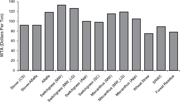
FIGURE 4-1 Biomass supplier WTA per dry ton projected by BioBreak model.
NOTE: Baseline scenario (no policy incentives, $111/barrel oil, 70 gallons per dry ton).
WTA
Given the parameter assumptions and an oil price of $111 per barrel, the biomass supplier’s average cost or WTA per ton of biomass delivered to the biorefinery ranges between $75 per dry ton for wheat straw in the Pacific Northwest to $133 per dry ton for switchgrass grown on high-quality land in the Midwest. Figure 4-1 provides the supply cost per dry ton for all 13 feedstock-rotation combinations in the analysis.11 Regional characteristics play a significant role. Switchgrass and Miscanthus grown on high-quality Midwest cropland have relatively high costs because of high land opportunity costs and lower yields relative to the Appalachian and South Central regions.
BioBreak derives the price gap between the biomass producer’s supply cost and the processor’s derived demand for biomass delivered to the biorefinery. Table 4-1 provides the biofuel processor’s WTP, biomass supplier’s WTA, and the price gap given the parameter assumptions and no policy incentives (for example, no blender’s tax credit or supplier payment).
This analysis ignores that RFS2, which requires that any cellulosic biofuel produced up to the mandated quantity be consumed, could influence feedstock producers and investors’ decision-making. Indeed, suppliers might be willing to invest in biofuel facilities irrespective of the economics described here if the consumption mandate of RFS2 is perceived as being rigid because the mandate provides a market for the biofuel. If the mandate is not perceived as being rigid, it will be difficult to induce private-sector investment. The complexities in the mechanisms for renewable identification numbers (RINs) for cellulosic
______________
11 The parameter draws and calculations were repeated 10,000 times resulting in 10,000 values for WTP, WTA, and the difference value (WTP-WTA) for each scenario. The value provided is the mean over the 10,000 calculations for each feedstock.
TABLE 4-1 BioBreak Simulated Mean WTP, WTA, and Difference per Dry Ton Without Policy Incentives
| WTA | WTP | WTA-WTP (per dry ton) | Price Gap in Dollars per Gallon of Ethanol | Price Gap in Dollars per Gallon of Gasoline Equivalent | |
| Stover (CS) | $92 | $25 | $67 | $0.96 | $1.43 |
| Stover-Alfalfa | $92 | $26 | $66 | $0.94 | $1.42 |
| Alfalfa | $118 | $26 | $92 | $1.31 | $1.97 |
| Switchgrass (MW) | $133 | $26 | $106 | $1.51 | $2.28 |
| Switchgrass (MW_LQ) | $126 | $27 | $99 | $1.41 | $2.13 |
| Switchgrass (App) | $100 | $26 | $74 | $1.06 | $1.59 |
| Switchgrass (SC) | $98 | $26 | $72 | $1.03 | $1.53 |
| Miscanthus (MW) | $115 | $26 | $89 | $1.27 | $1.90 |
| Miscanthus (MW_LQ) | $119 | $27 | $93 | $1.33 | $1.98 |
| Miscanthus (App) | $105 | $27 | $79 | $1.13 | $1.69 |
| Wheat Straw | $75 | $27 | $49 | $0.70 | $1.04 |
| SRWC | $89 | $24 | $65 | $0.93 | $1.39 |
| Forest Residues | $78 | $24 | $54 | $0.77 | $1.16 |
NOTE: Oil price is assumed to be $111 per barrel and conversion efficiency of biomass to fuel is assumed to be 70 gallons per dry ton.
biofuels could lead investors to conclude the cellulosic mandate is not rigid (see Chapter 6 for further discussion of RINs).
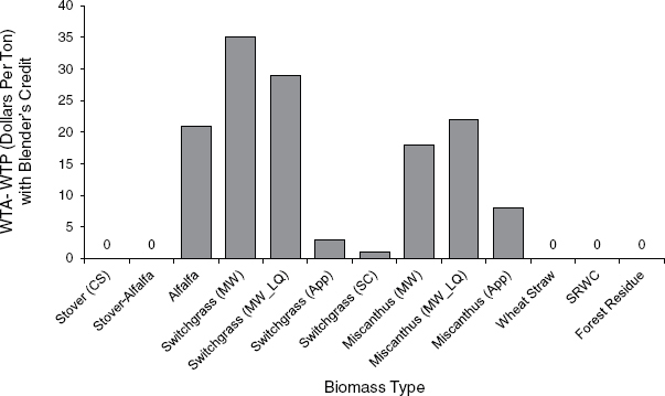
Without policy intervention, no feedstock market is feasible in economic terms in the baseline scenario. The price gap that would need to be closed to sustain a feedstock market ranges between $49 per dry ton for wheat straw to $106 per dry ton for switchgrass grown on high-quality land in the Midwest. Figure 4-2 provides a graphical depiction of the price gap for all 13 feedstock-rotation combinations (see also Box 4-3).
The breakeven values and resulting price gaps depicted in Figure 4-2 are sensitive to assumptions and parameters used in the analysis. One key parameter in the BioBreak model is the price of oil (see Box 4-1). The price of oil drives the processor’s derived demand for feedstock given biomass conversion cost and influences biomass supply cost through production costs. An increase (decrease) in the price of oil increases (decreases) what the processor can pay per dry ton of each feedstock and break even in the long run. At the same time, an increase (decrease) in the oil price increases (decreases) harvest and transportation costs resulting in a higher (lower) biomass supplier long-run breakeven cost. Given the assumptions, the effect on the processor’s derived demand price from an oil price change dominates the effect on the biomass supply cost. Therefore, the price gap (WTA – WTP) decreases with higher oil prices and vice versa.
The results in Table 4-1 and Figures 4-1 and 4-2 assume an oil price of $111 per barrel. At an oil price of $191 per barrel, the price gap is eliminated for several feedstocks, including stover (CS), switchgrass (App, SC), Miscanthus (App), wheat straw, SRWC, forest residue, and stover-alfalfa. Remaining feedstocks have a price gap between $5 and $23 per dry ton. Correspondingly, the price gap increases to between $110 and $168 per dry ton of biomass with an oil price of $52 per barrel. The breakeven price is also sensitive to the conversion rate of biomass to ethanol. The baseline results assume a conversion rate of 70 gallons per dry ton
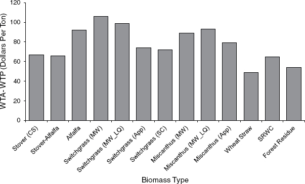
FIGURE 4-2 Gap between supplier WTA and processor WTP projected by BioBreak model.
NOTE: No policy incentives (WTA – WTP, $111 per barrel oil, 70 gallons per dry ton).
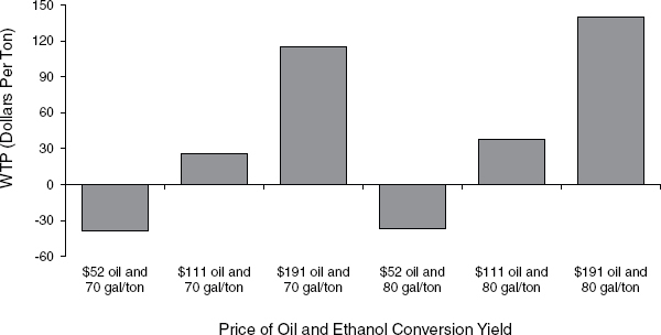
of biomass for all types of feedstocks (see Box 4-1), but potential advances in the conversion process may increase this rate. An increase in the biomass conversion rate increases the biorefinery returns per unit of feedstock converted and therefore reduces the price gap. Figure 4-4 provides sensitivity results of the processor WTP for South-Central switchgrass to the price of oil and conversion rate. Sensitivity results for other feedstocks are similar.
The results presented above assume no policy incentives. Any policy incentives for either the processor or supplier will decrease the price gap needed for market viability. The 2008 farm bill provides a $1.01 per gallon tax credit to cellulosic biofuel blenders. Figure 4-5 displays the price gap when the blender’s credit is included. Given the blender’s tax credit, the price gap drops significantly, resulting in viable feedstock markets for stover (CS), stover-alfalfa, wheat straw, SRWC, and forest residues (that is, WTP > WTA or WTA – WTP < 0). The remaining feedstocks have a gap between $1 and $35 per dry ton. Similarly, any policy incentive to suppliers, such as the U.S. Department of Agriculture’s (USDA’s) Biomass Crop Assistance Program in the 2008 farm bill, which provides payments for establishing bioenergy crops and collecting biomass, would further decrease the price gap and, given BioBreak’s baseline assumptions, result in viable feedstock markets for all feedstocks in the analysis (for more on the Biomass Crop Assistance Program, see Box 4-4 in section “Potential Changes Caused by Biofuel Policy”). Policy incentives for carbon emissions could also affect the price gap (as discussed later in the section “Interaction of Biofuel Policy with Possible Carbon Policies”).
One benefit of using Monte Carlo simulation to derive the breakeven values is the ability to capture the variability found in the literature for each parameter in the model. For the BioBreak application presented here, the Monte Carlo simulation was conducted using
BOX 4-3
Gap in Forest Residue Demand and Supply
The market for forest residue exemplifies the gap between WTP and WTA for cellulosic feedstock. Many existing studies assume that a large proportion of wood will be available for cellulosic ethanol production through harvesting of residues. However, these studies often ignore the likely costs of extracting residues. Figure 4-3 shows that, in most cases, forest residues are not collected because the costs of extracting additional residues are likely to be high relative to the value. Figure 4-3 also shows the marketable components of a typical tree. The bole of the tree is the main marketable log from the stump at the bottom up to a diameter of 7 inches or so. This material typically is cut into lumber of some sort, depending on the form of the tree. From 7 inches or so up to around 4 inches, the main log of the tree is likely used as pulpwood. The additional stems at the top of the tree, the branches, and the leaves have traditionally been left as slash in the forest. The reason these components have been left as slash is largely economic—the cost of extracting this additional material is greater than the value of selling it. As shown in the right hand side of Figure 4-3, WTP for sawtimber is typically much higher than the marginal cost of extracting the large stems. WTP for extracting pulpwood, however, is close to, or equal to, the marginal cost of extracting the pulp component of timber, and WTP for biomass material is less than the marginal cost of extracting the additional material.
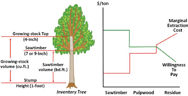
FIGURE 4-3 Components of trees and their use and value in markets.
NOTE: Sawtimber represents the largest part of the stump, up to about 9 inches in diameter. Pulpwood represents the rest of the stump up to 4 inches. The remainder is residue (often referred to as “slash”).
SOURCE: Adapted from Figure 8 in Perlack et al. (2005).
10,000 draws from the assumed distribution for each parameter. From each draw, WTA, WTP, and the price gap were calculated for each feedstock. The results presented so far have been the mean values over all 10,000 calculations. Using the distributional assumptions outlined in Appendix L, which are based on literature summarized in Appendix M, Table 4-2 provides the estimated WTA value for each feedstock at select percentiles over the 10,000 Monte Carlo simulations at an oil price of $111 per barrel. The values in Table 4-2 provide a sensitivity range for the breakeven feedstock supply cost based on the parameter variation found in the literature.
NOTE: WTA – WTP under the assumptions of $111 per barrel of oil and a biomass to fuel conversion efficiency of 70 gallons per dry ton.
TABLE 4-2 BioBreak Simulated WTA Value Without Policy Incentives by Percentile
| 10% | 25% | 40% | MEAN | 60% | 75% | 90% | |
| Stover (CS) | $81 | $87 | $91 | $92 | $95 | $97 | $101 |
| Stover-Alfalfa | $87 | $89 | $91 | $92 | $93 | $95 | $97 |
| Alfalfa | $114 | $116 | $118 | $118 | $119 | $120 | $122 |
| SG (MW) | $109 | $118 | $125 | $133 | $135 | $144 | $159 |
| SG (MW_LQ) | $115 | $121 | $124 | $126 | $128 | $132 | $136 |
| SG (App) | $87 | $93 | $97 | $100 | $102 | $107 | $115 |
| SG (SC) | $85 | $90 | $93 | $98 | $98 | $103 | $112 |
| Misc (MW) | $102 | $109 | $113 | $115 | $118 | $122 | $127 |
| Misc (MW_LQ) | $99 | $107 | $113 | $119 | $121 | $129 | $142 |
| Misc (App) | $91 | $98 | $103 | $105 | $108 | $113 | $119 |
| Wheat Straw | $65 | $70 | $73 | $75 | $77 | $80 | $86 |
| Farmed Trees | $78 | $83 | $86 | $89 | $91 | $94 | $100 |
| Forest Residue | $68 | $73 | $76 | $78 | $80 | $83 | $88 |
NOTE: Oil price is assumed to be $111 per barrel and conversion efficiency of biomass to fuel is assumed to be 70 gallons per dry ton.
Comparing Feedstock Cost Estimates of the BioBreak Model with Other Studies
The cost estimates generated by the model are highly dependent on the assumptions used and the parameters considered. The way costs are treated and the comprehensiveness of which economic costs are included in the biomass supply chain and in ethanol processing varies by study. For example, the U.S. Billion-Ton Update: Biomass Supply for a Bioenergy and Bioproducts Industry (Perlack and Stokes, 2011) relies on the University of Tennessee’s POLYSYS modeling system to estimate the marginal cost for supplying biomass to range from $40-$60 and average about $50 per dry ton of harvested biomass at the farm gate. BioBreak costs for wheat straw to the farm gate average about $40 per dry ton, corn stover about $55-$60 per dry ton, and switchgrass in the Appalachian and South Central Regions about $65 per dry ton without land opportunity costs included and $80 with land opportunity costs. Preliminary results indicate that much of the switchgrass would be produced on converted pasturelands that would have low opportunity costs. Handling, possibly drying, storing, and transporting low-density dry biomass to the biorefinery is a logistical challenge and costly (see Chapter 6).
Another study by Khanna et al. (2010) developed costs of production for corn stover, wheat straw, Miscanthus, and switchgrass for a number of potential producing states and then used these costs of production to develop biomass supply curves. Again, these were comprehensive costs at the farm gate that included land opportunity costs and were developed for the low-cost scenario assuming the availability of CRP land on which to produce switchgrass and Miscanthus. Farm-gate low-cost scenario estimates ranged from $44 to over $110 per dry ton for Miscanthus and $55 to $105 per dry ton for switchgrass. The high-cost scenarios were higher than those reported for BioBreak above. Corn stover estimates ranged from a low of $63 for no-till CS rotation to a low of $99 per dry ton for conventional till with median values of over $110 per dry ton for both CS tillage options. Again, the costs reported from the Khanna et al. (2010) did not include costs beyond the farm gate for transportation and storage.
The biomass cost estimates derived using the BioBreak model are typically higher than most similar studies because the model is inclusive of all economic costs (including opportunity costs of land) involved in producing, harvesting, storing, and delivering the last dry ton of biomass to the biofuel processing facility through the biomass supply chain.
Likewise, the biomass conversion costs account for all long-run costs in processing biomass to ethanol and include coproduct returns from a biorefinery of given capacity.
Finally, most studies assume biomass production costs are independent of crude oil prices; however, there are two factors that cause biomass production costs to increase as crude oil prices increase. First, part of the variability in crude price is due to the value of the dollar relative to other currencies. This same effect has been shown to influence crop prices (Abbott et al., 2009). Any increase in crude price caused by a devalued dollar would also increase opportunity costs for the land and fuel-based biomass production costs. It would also raise the demand for biofuels. Second, a portion of the cost of harvest, transportation, and nutrient replacement is related to the cost of fossil fuels. This concurrent increase in biomass cost would increase the apparent crude price at which biofuels would become cost competitive. The BioBreak model has attempted to incorporate these price effects on WTA.
Cost of Converting Cellulosic Biomass to Liquid Fuels
As mentioned earlier, along with the cost of harvesting and transporting biomass to a biorefinery is the cost of converting it into fuel. No commercial-scale facilities currently exist for the production of liquid fuels from cellulosic biomass. The conversion cost data used in the BioBreak analysis are based on laboratory or pilot-scale performance information and estimated investment and operating cost data for an optimized nth biorefinery that uses biochemical conversion of corn stover to ethanol (Aden et al., 2002). A recent report by Anex et al. (2010) compared the cost to produce liquid biofuels biochemically and thermochemically. The report examined the costs of fermentation to produce ethanol, fast pyrolysis to produce a gasoline or diesel “drop-in” fuel, and gasification and Fischer-Tropsch (F-T) to produce a gasoline or diesel “drop-in” fuel. Because the three technologies produce fuels with different energy contents, the results are presented in terms of gallons of gasoline equivalent. RFS2 is written in terms of gallons of ethanol equivalent, so a lesser volume of “drop-in” fuels from pyrolysis or F-T based technologies are required to satisfy RFS2. (See Table 1-1 in Chapter 1.) The study was based on a consistent biorefinery size of 2,205 dry tons per day of corn stover. All capital and operating costs are referenced to 2007. Corn stover is priced at $75 per dry ton, delivered to the biorefinery on a year-round basis. The only significant products from the biorefinery are the liquid fuel and electricity or gaseous fuel generated from the unconverted biomass. A required selling price for the liquid fuel is calculated to give a 10-percent discounted cash flow rate of return on a fully equity-financed project with a 20-year life.
The cellulosic ethanol costs in the paper were based on the equipment in a 2002 study by the National Renewable Energy Laboratory (NREL) (Aden et al., 2002), updated to 2007 construction and cellulase costs. The Anex et al. study (2010) used a nominal ethanol yield of 68 gallons per dry ton of biomass, which was the maximum demonstrated yield at the time the study was conducted and is close to the yield that this committee uses in the BioBreak analysis.
The gasification and F-T economics in Anex et al. (2010) are based on an NREL report prepared by Swanson et al. (2010). Two cases were evaluated: A high-temperature (HT), entrained flow, slagging gasification system and a lower temperature, fluidized bed, non-slagging gasification system. The HT system produces more fuel per ton of biomass, but its capital cost is higher. Overall cost to produce is slightly lower for the HT case because of the higher liquid yield. Biomass gasification has been attempted by several groups at
the pilot scale. Operational difficulties have been encountered, but the gasification and F-T technology are well established for coal. Therefore, the cost data and yields for the gasification and F-T scheme can be considered reasonably reliable once the operational difficulties are overcome.
The fast pyrolysis economics are based on Wright et al. (2010). Fast pyrolysis of biomass for fuel production is a relatively new technology with little published information on yields, potential operational problems, or required equipment. The process uses equipment that is common in the petroleum refining industry, such as hydroprocessing, hydrocracking, hydrogen production, and high-temperature solids circulation similar to the fluid catalytic cracking process.
Kior, a privately funded company that is developing catalytic pyrolysis technology, submitted a Form S-1 to the U.S. Securities and Exchanges Commission (Kior, 2011) that contained additional information on capital requirements and overall yields. The technology and equipment proposed by Kior are similar to that used in the Wright et al. (2010) study, except that Kior has included a boiler and turbogenerator system to convert the off-gas and excess char into electricity. The capital costs included in Wright et al. were much lower than those reported by Kior. Although the boiler and turbogenerator represent a large capital investment, they are required to recover the energy contained in the nonliquid products as in the case of ethanol biorefineries. The Kior capital estimate is for a first-of-its-kind facility and its current usage is closer to an nth plant than a pioneer plant, but it is based on a fully developed cost estimate prepared by a major engineering company. In contrast, Wright et al.’s cost estimate is a “scoping quality” estimate for a fully developed technology. When adjusted to the same feed rate using a 0.6 scaling factor, capital cost estimated by Wright et al. was 43 percent of the capital cost estimated by Kior. Wright et al. (2010) acknowledged that some aspects of technology, such as solids removal from the pyrolysis oil, have yet to be developed and demonstrated.
The cases reported by Wright et al. (2010) and Kior (2011) were evaluated. The raw pyrolysis oil has to be hydrotreated before it can be used as a fuel. The two cases in Wright et al. (2010) differ in the source of hydrogen used to hydrotreat the pyrolysis oil. In the first case, part of the pyrolysis oil is used as feedstock to an on-site hydrogen plant to produce hydrogen. In the second case, hydrogen is purchased from an off-site plant that uses natural gas to produce the hydrogen. Producing hydrogen on site from bio-oil product lowers the liquid yield and increases the capital cost for the project. Kior’s case is similar to the hydrogen purchase case by Wright et al. (2010), with the exception of the capital costs (as discussed earlier) and yield estimates.
The pertinent information from the published studies is summarized in Table 4-3 along with a calculation of the number of biorefineries and capital investment required, the number of acres of land necessary to produce the biomass (assuming all biomass for bioenergy comes from dedicated bioenergy crops), and the annual subsidies that would be required to support the industry at various crude oil prices. Table 4-3 demonstrates that catalytic pyrolysis and fast pyrolysis are promising technologies; they can produce “drop-in” products that are compatible with the existing petroleum distribution system. However, pyrolysis still requires substantial research and development before it is economically viable without subsidies.
The three crude prices used in Table 4-3 to calculate subsidies are from the three crude price scenarios for 2022 listed in the 2010 Annual Energy Outlook (EIA, 2010a). Only the high crude price scenario eliminates the need for subsidies to support a biofuel industry. All other price scenarios require either subsidies for the biofuel industry or additional taxes on petroleum products to narrow the price gap between petroleum fuels and biofuel. Without
TABLE 4-3 Summary of Economics of Biofuel Conversion
| Ethanol | Gasification and F-T | Pyrolysis, Hydrogen Purchase | ||||
| 90 Gallons Per Dry Ton |
70 Gallons Per Dry Ton |
High Temp | Low Temp | High Yield | Kior | |
| Single Plant Capital, Million Dollars | 380 | 380 | 606 | 498 | 200 | 463 |
| Fuel Produced, Million Gallons Per Year | ||||||
| Million Gallons Per Year | 69.5 | 52.4 | 41.7 | 32.3 | 58.2 | 43.1 |
| Million Gallons of Gasoline | 46.3 | 34.9 | 41.7 | 32.3 | 58.2 | 48.9 |
| Equivalent Per Year | ||||||
| Cost to Produce | ||||||
| Nth Plant | 375 | 500 | 430 | 480 | 210 | 324 |
| Pioneer Plant | 650 | 850 | 800 | 750 | 350 | N/A |
| Number of Plants to Meet 16 billion gallons of ethanol-equivalent biofuels in 2022 | 230 | 305 | 256 | 331 | 183 | 218 |
| Capital Costs Required to Meet RFS2, Billion Dollars | 88 | 116 | 155 | 165 | 37 | 101 |
| Price Gap, Billion Dollars Per Year | ||||||
| At $52 Per Barrel | 25 | 39 | 31 | 37 | 8 | 20 |
| At $111 Per Barrel | 10 | 24 | 16 | 21 | -7 | 5 |
| At $191 Per Barrel | -10 | 3 | -4 | 1 | -28 | -16 |
| Biomass Feed Requirements | ||||||
| Million Dry Tons Per Year | 178 | 236 | 175 | 226 | 133 | 159 |
| Million Acres at 5 Tons Per Acre | 36 | 47 | 35 | 45 | 27 | 32 |
SOURCES: Aden et al. (2002); Anex et al. (2010); R. Anex (University of Wisconsin, Madison, personal communication on August 23, 2011); Swanson et al. (2010); Wright et al. (2010).
these subsidies or taxes, the biofuel industry would not expand to meet RFS2 requirements. An increase of $25 per dry ton in the price of biomass increases the annual subsidies required by $5 billion to $10 billion per year. Figure 4-6 shows a graphical breakdown of the production costs.
The capital-related costs in Figure 4-6 include the average depreciation and the assumed 10-percent return on investment for the 20-year life of the project. In the discounted cash flow analysis used to develop these costs, the capital charges are higher in the early years of the project and decline throughout the life of the project. The per-gallon, capital-related operating costs are determined by dividing this average annual effective cost of capital (depreciation plus return on investment) by the annual fuel production. The annual effective cost of capital varies from 12 to 14 percent of the total capital investment for the various projects. Another way of defining these costs is to assume they are an effective capital recovery factor for the capital investment. This range of capital recovery factors would give an effective rate of return of about 12 percent for a 20-year project.
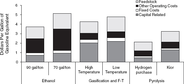
FIGURE 4-6 Breakdown of biomass conversion costs.
The 10-percent after-tax rate of return used in these studies is probably on the low side of returns that would be required to attract capital for a new, high-risk project. The economics also assume that the project is fully equity financed. None of these projects has yet to be demonstrated commercially, implying that they are high-risk investments. High-risk investments usually require higher returns or leveraging (borrowing) of capital to reduce the risk. Either of these would increase the effective cost of capital for at least the early projects, so the total production cost numbers are probably low.
The costs in Table 4-3 and Figure 4-6 are pre-tax wholesale costs at the biorefinery gate. “Drop-in” fuels, such as those produced by pyrolysis and gasification and F-T, can use the existing petroleum infrastructure for delivery to the final consumer. Transportation and distribution costs for drop-in fuels would be similar to current petroleum products transportation costs of $0.02-$0.05 per gallon. Cellulosic ethanol would continue to be shipped by rail, barge, and truck for blending at the final distribution point with costs of $0.10-$0.50 per gallon. Construction of an ethanol pipeline system would reduce transportation costs but would require additional capital investment. Nominal pipeline construction costs typically exceed $1 million per mile (Smith, 2010).
Producing enough biomass to meet RFS2 could require 30-60 million acres of land, excluding the high yield, hydrogen-purchase pyrolysis case in Table 4-3. If all biomass for cellulosic biofuels is produced from dedicated energy crops, the amount of land needed would be at the high end of the estimate. The use of corn stover, wheat straw, other crop residues, and forest residues would reduce the amount of acres needed.
PRIMARY MARKET AND PRODUCTION EFFECTS OF U.S. BIOFUEL POLICY
Because RFS2 creates another market for crops, particularly for corn, and a possible incentive to shift land from food crops to biomass feedstocks, the mandate has repercussions for related commodity markets. The prices of grain and oilseed crops, food, animal feed, and wood products have all experienced upward pressure coinciding with the rapid expansion of the biofuel market. Coproducts from biofuel have also introduced competition in feed
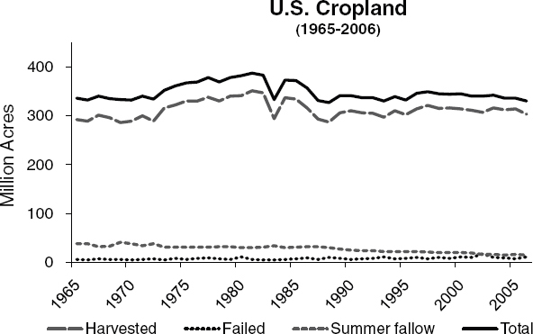
FIGURE 4-7 Allocation and use of U.S. cropland from 1965 to 2006.
DATA SOURCE: USDA-ERS (2007).
markets. Increasing biofuel in the transportation fuel market could affect domestic gasoline and diesel prices. Demand for feedstocks to meet traditional needs and those of the biofuel market increases competition for land. Although several attempts have been made to tie price and resource use effects to biofuel expansion, there is little agreement in the economic literature about the effects that can be attributed to biofuel expansion. Therefore, this section presents what has happened recently to resource prices and use relative to biofuel expansion rather than a cause-and-effect empirical analysis of biofuel expansion.
Agricultural Commodities and Resources
This section reviews the primary feedstuff and food crops, market series, and cropland resource base published by the U.S. Department of Agriculture (USDA) National Agricultural Statistics Service (NASS). Figure 4-7 provides an indication of what has happened over time to total cropland and total harvested cropland. Both series peaked in 1981 and have slowly trended downward through 2006 to about 300 million acres, with reportedly a slight increase since 2006. There has been concern over land-use change associated with the expansion of the biofuel industry. The continuous reallocation of existing cropland along with productivity growth has supported increased output even though overall cropland acres are decreasing in the United States. However, that may not be the case in other parts of the world.
Changes in production levels follow changes in demand for and net returns to certain crops. The major field crops in terms of harvested acreage are corn, soybean, wheat, and hay (Figure 4-8). As Figure 4-8 indicates, domestic acreage for corn and soybean has been increasing, hay acreage has been relatively constant, and wheat acreage has been declining.
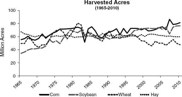
FIGURE 4-8 Harvested acres of corn for grain, soybean (all), wheat, and hay (all) from 1965 to 2009.
DATA SOURCE: USDA-NASS (2010).
These adjustments are in response to differences in relative commodity prices and differences in yield and productivity growth affecting net returns on these crops over time.
When considering agricultural commodity prices over time, media sources frequently refer to nominal prices, abstracting from the temporal impacts of inflation on prices. Although substantial nominal price shocks occurred in the mid-1970s and again in the beginning of 2006, it is important to remove inflationary impacts on prices or to convert from nominal to real prices by using an appropriate deflator as presented in Figure 4-9. Despite short-run price shocks, real commodity prices have been decreasing over the long run as a result of total factor productivity growth in the agricultural sector. Real price shocks for corn, soybean, and wheat were concurrent with higher oil real prices in the mid-1970s. Beginning in 2006, real commodity prices have tended to demonstrate increased fluctuation but modest overall increases.
Several attempts have been made to link real price changes to increased feedstock demand for biofuels, but results vary significantly between studies (see also the section “Food Prices” later in this chapter). U.S. demand for corn as an ethanol feedstock accounts for more than 40 percent of crop use (even though one-third of the grain weight is returned as a feedstuff source in dried distillers grains with solubles [DDGS]). All other things equal, corn prices will increase if there is increased corn demand for ethanol production. However, the magnitude of the price effect is not clearly established (see also “Effect of Short-term Price Spikes on Livestock Producers” in this chapter) and depends on several factors, such as biofuel expansion, drought, flooding, crop failures, exchange rate shifts, government price supports, and trade restrictions. In the short run, increased corn feedstock demand may cause a substantial corn price shock, but, in the long run, production resources will shift to increase corn supply and moderate price increases.
Figures 4-10 and 4-11 provide an indication of how production has shifted in the United States in the three major commodity crops from the 1965 to 2010 crop years. The production
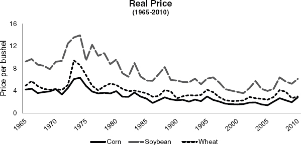
FIGURE 4-9 Real prices for corn, soybean, and wheat from 1965 to 2010 crop year.
NOTE: 1990-1992=100.
DATA SOURCE: Price index for Producer Prices Paid Index from USDA-NASS and USDA-ERS.
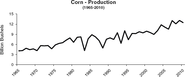
FIGURE 4-10 U.S. corn-grain production from 1965 to 2010 crop year.
DATA SOURCE: USDA-NASS (2010).
of corn and soybean has been increasing significantly over time, while wheat production peaked in 1981 and has been slowly declining, although with significant annual fluctuation up to the 2010 crop year.
At the same time, Figure 4-12 indicates that domestic consumption of corn has increased significantly. The increase in corn production began in 1975 (well before the demand for biofuel). Thus, in addition to the demand for biofuel, the increase in domestic consumption of corn can be attributed to increases in feed and residual use (USDA-NASS, 2010). Domestic consumption of soybean, possibly affected by the demand for soybean
oil as a biodiesel feedstock, has held steady. Domestic wheat consumption has remained relatively flat in recent years.
Another perspective on how biofuel production is affecting the domestic and global markets is to view patterns in U.S. net exports of corn, soybean, and wheat. It could be argued that net exports would decline, especially with increasing domestic consumption of corn, and to a lesser extent of soybean oil, for biofuel feedstock. Figure 4-13 indicates that
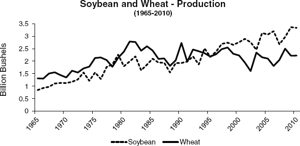
FIGURE 4-11 U.S. soybean and wheat (all) production from 1965 to 2010 crop year.
DATA SOURCE: USDA-NASS (2010).
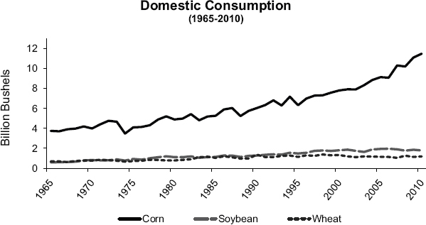
FIGURE 4-12 U.S. domestic consumption of corn, soybean, and wheat from 1965 to 2010 crop year.
DATA SOURCE: USDA-NASS (2010).
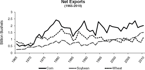
FIGURE 4-13 U.S. net exports of corn, soybean, and wheat from 1965 to 2010 crop year.
NOTE: Total year exports minus total year imports.
DATA SOURCE: USDA-FAS (2010).
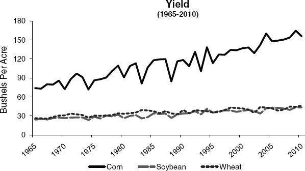
FIGURE 4-14 Annual yields for corn grain, soybean, and wheat from 1965 to 2010 crop year.
DATA SOURCE: USDA-NASS (2010).
net corn exports have held fairly steady, net soybean exports have actually increased, and wheat exports have declined, while yields have been steadily increasing for all three crops, as shown in Figure 4-14.
What accounts for the increase in corn and soybean production and the gradual decline in wheat production? Essentially, market forces determine the allocation of resources.
Producers select the most profitable combination of crops to produce on the cropland acres they farm. The prices, yields, seed technology, and government programs make corn and soybean more profitable than wheat. In addition, income improvement and diet adjustments in developing countries create growing demand for feed grains and oilseeds to produce animal products as well as biofuels.
In summary, the committee made the following observations on what is happening in U.S. agricultural commodity markets and resource use. First, cropland acreage has been declining slowly over time. Second, shifts in acreage for grain and oilseed crops were under way before the advent of biofuel expansion even though biofuel expansion and growing export demand have encouraged the shift in recent years.
Food Prices
The diversion of land to corn production and a greater demand for corn from the biofuel industry discussed in the previous section coincided with an aberrant rise in food prices in the mid-2000s. Between 2004 and 2008, the price of the staple commodities (wheat, corn, soybean, and rice) grew an average of 102 percent (Figure 4-15) (IMF, 2010). Even though real prices had been at an all-time low in the late 1990s and early 2000s (Babcock et al., 2010), the rapid nature of the increase was disruptive to food processors and to households. The Food Consumer Price Index (CPI), calculated by USDA’s Economic Research Service, increased from 2.4 percent in 2006 to 4 percent in 2007 and grew a further 5.5 percent in 2008 (USDA-ERS, 2011b). Food banks and international development organizations expressed
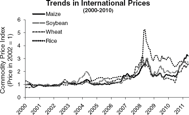
FIGURE 4-15 Trends in real international prices of key cereals: 1960 to May 2008.
SOURCE: Adapted from Abbott et al. (2011).
particular concern for households that allocated a large percentage of income to food (Crompton, 2008; Lustig, 2008; Reinbold, 2008; von Braun, 2008; Wiggins and Levy, 2008).
During this commodity price spike, which peaked between 2007 and 2009, controversy ensued over the role of increased ethanol production in increased food prices. However, much of the debate used the term “food prices” in an imprecise and often contradictory manner. Specifically, some analysis of that period focused on the effect of ethanol production on raw agricultural commodity prices at either the farm level or the international market level. Other analysis focused on the effect of ethanol production on prices of processed food products at the consumer retail level. Frequently, both types of analysis were reported to the public under the label of “the effect on food prices.”
As discussed below, the nature of the U.S. food marketing system implies that changes in agricultural commodity prices and changes in retail food product prices do not correlate on a 1:1 basis. Much of the confusion in that debate, and the wide range of estimated effects of ethanol production on “food prices” during that period, was due to these uses of imprecise terminology. Consequently, the remainder of this section uses specific terminology to discuss the potential price effects of expanded biofuel production. First, the term “agricultural commodity prices” refers to the prices of raw agricultural products at the farm or international market level. Second, the term “retail food prices” refers to the prices of consumer food products at the grocery retail level.
Effects on Agricultural Commodity and Retail Food Prices: Lessons from 2007-2009
Estimates of ethanol’s influence on global agricultural commodity prices during the 2007-2009 period were as high as 70 percent (Table 4-4). Determining the extent to which biofuel production affected agricultural commodity and retail food prices is difficult because most prices at the time were also influenced by the high price of oil, greater speculation activity in commodity markets, the changing value of the dollar relative to other currencies, drought in some major production regions, export restrictions imposed by some countries, and more demand for food from the growth in population and incomes in developing countries (Trostle, 2008; Baffes and Haniotis, 2010). Some combination of these events is likely to continue to influence prices. Though the increase in the Food CPI dropped to historically low levels (1.8 percent for 2009 and 0.8 percent for 2010, the lowest rate since 1962 [USDA-ERS, 2011b]), food prices are still much higher than they were at the beginning of the decade (IMF, 2010), and food inflation in 2011 is projected to return to the historic average of between 2 and 3 percent (USDA-ERS, 2011b).
Furthermore, because of the interrelationships of agricultural commodity markets and the competition for production resources among agricultural commodities, a price change in one agricultural commodity can affect prices in other agricultural commodity markets (see “Agricultural Commodities and Resources” above). Thus, any secondary price effect needs to be taken into account in the analysis of the effects of ethanol on commodity or retail prices. Also, the magnitude of price changes at the farm, international market, or retail level resulting from increased ethanol production is determined by the complex nature of the food marketing system and the transmittal of price changes through that system. Thus, though price changes at each level of the food system are jointly determined, the size of the price changes at each level may differ.
The range of agricultural commodity price increases assigned to increased ethanol production tended to decrease with the passage of time as additional data became available and more accurate analysis could be conducted (Abbott et al., 2009; Baffes and Haniotis,
TABLE 4-4 Estimates of Effect of Biofuel Production on Agricultural Commodity Prices, 2007-2009
| Author | Coverage and Key Assumptions | Key Effects of Biofuels on Agricultural Commodity Prices |
| Banse et al. (2008) | 2001-2010; Reference scenario without mandatory biofuel blending, 5.75% mandatory blending scenario (in EU member states), 11.5% mandatory blending scenario (in EU member states) | Price change under reference scenario, 5.75% blending and 11.5% blending, respectively: Cereals: –4.5%, –1.75%, +2.5% Oilseeds: –1.5%, +2%, +8.5% Sugar: –4%, –1.5%, +5.75% |
| Baier et al. (2009) | 24 months ending June 2008; historical crop price elasticities from academic literature; bivariate regression estimates of indirect effects | Global biofuel production growth responsible for 17%, 14%, and 100% of the rises in corn, soybean, and sugar prices, respectively, and 12% of the rise in the IMF’s agricultural commodity price index. |
| Lazear (2008) | 12 months ending March 2008 | U.S. ethanol production increase accounted for 33% of the rise in corn prices. U.S. corn-grain ethanol production increased global food prices by 3%. |
| IMF (2008) | Estimated range covers the plausible values for the price elasticity of demand | Range of 25-45% for the share of the rise in corn prices attributable to ethanol production increase in the United States. |
| Collins (2008) | 2006/07-2008/09; Two scenarios considered: (1) normal and (2) restricted, with price inelastic market demand and supply | Under the normal scenario, the increase in ethanol production accounted for 30% of the rise in corn price. Under the restricted scenario, ethanol could account for 60% of the expected increase in corn prices. |
| Glauber (2008) | 12 months ending April 2008 | Increase in U.S. biofuels accounted for about 25% of the rise in corn prices; U.S. biofuel production accounted for about 10% of the rise in IMF global agricultural commodity price index. |
| Lipsky (2008) and Johnson (2008) | 2005-2007 | Increased demand for world biofuels accounts for 70% of the increase in corn prices. |
| Mitchell (2008) | 2002–mid-2008; ad hoc methodology: effect of movement in dollar and energy prices on food prices estimated, residual allocated to the effect of biofuels | 70-75% of the increase in agricultural commodities prices was due to world biofuels and the related consequences of low grain stocks, land use shifts, speculative activity, and export bans. |
| Abbott et al. (2009) | Rise in corn price from about $2 to $6 per bushel accompanying the rise in oil price from $40 in 2004 to $120 in 2008 | $1 of the $4 increase in corn price (25%) due to the fixed subsidy of $0.51 per gallon of ethanol. |
| Rosegrant (2008) | 2000-2007; Scenario with actual increased biofuel demand compared to baseline scenario where biofuel demand grows according to historical rate | Increased biofuel demand is found to have accounted for 30% of the increase in weighted average grain prices, 39% of the increase in real maize prices, 21% of the increase in rice prices, and 22% of the rise in wheat prices. |
| Fischer et al. (2009) | (1) Scenario based on the IEA’s WEO 2008 projections; (2) variation of WEO 2008 scenario with delayed 2nd generation biofuel deployment; (3) aggressive biofuel production target scenario; (4) variation of target scenario with accelerated 2nd generation deployment | Increase in prices of wheat, rice, coarse grains, protein feed, other food, and nonfood, respectively, compared to reference scenario: (1) +11%, +4%, +11%, –19%, +11%, +2% (2) +13%, +5%, +18%, –21%, +12%, +2% (3) +33%, +14%, +51%, –38%, +32%, +6% (4) +17%, +8%, +18%, –29%, +22%, +4% |
SOURCE: Timilsina and Shrestha (2010).
2010; Timilsina and Shrestha, 2010).12 In addition, given the wide range of scenarios used by the authors summarized in Table 4-4 and the level of uncertainty about future scenarios, a precise estimate of the effect of expanded biofuel production on agricultural commodity prices is likely to be impossible. Instead, a range of possible price effects during 2007-2009 is probably most instructive in understanding the potential effect of biofuel production on agricultural commodity prices. For purposes of this analysis, a range of 20 to 40 percent increase in agricultural commodity prices is used.
The next step in analyzing the effect of expanded biofuel production on retail food prices is to convert the change in agricultural commodity prices (20-40 percent) into a change in retail grocery prices paid by consumers. This conversion depends critically on the size and nature of the marketing process between the farm level and the retail level. The cost of this process, typically defined as the “marketing margin” of food products, includes the cost of all processing, transportation, and distribution activities that occur between the sale of agricultural commodities at the farm level and the purchase of a consumer food product at the retail level. The marketing margin on an agricultural commodity is typically measured as “the difference between the price paid by consumers and that obtained by [farm-level] producers” for that quantity of the agricultural commodity contained in the consumer food product (Tomek and Robinson, 1983, pp. 120-122). To the extent that an agricultural commodity undergoes a greater degree of processing before reaching the final consumer or is costlier to transport and distribute, that agricultural commodity would have a greater marketing margin when measured as the share of the price paid by the consumer. Only if the marketing margin approaches zero would the full effect of an agricultural commodity price change be transmitted to the final consumer on a one-to-one basis (Gardner, 1975, 1987).
Those agricultural commodities most affected by the production of biofuels in 2007-2009 (primarily corn, soybean, and wheat) typically undergo a high degree of processing before reaching grocery consumers in the United States. Thus, the marketing margin on those agricultural commodities tends to be relatively high. Many corn-based consumer products (for example, corn flakes or corn syrup) had a marketing margin of 95 percent, while wheat-based consumer products (for example, bread or bakery products) had a marketing margin of approximately 90 percent, and soybean-based products (for example, shortening or margarine) had a marketing margin of 84 percent in 2006. On average, including all other food products, the marketing margin for all agricultural products has been approximately 81 percent in recent years (USDA-ERS, 2011c).
Consequently, in determining the increase in the consumer retail price of a food product that results from an increase in the price of the agricultural commodity contained in that food product, both the increase in the price of the agricultural commodity and the marketing margin of the consumer food product have to be considered. In the case of corn, for example, if the range of a 20 to 40 percent price increase for corn is used with a marketing margin of 95 percent, then the retail price of grocery food products containing corn would
______________
12 This section is based on the recent economic literature as of 2011 on the effect of ethanol production on agricultural commodity prices and retail food prices during 2007-2009. Much of the analysis conducted at that time suggested that the price effects of increased ethanol production were larger than the subsequent analysis. This is likely the result of the additional or improved data available to researchers during 2009-2010 and is not a reflection on the quality of the earlier analysis.
be a 1 to 2 percent increase in price at the retail level.13 In the case of animal products, the marketing margin is lower relative to other foods. In 2010, the marketing margins for chickens (broilers), pork, and beef averaged 58, 69, and 54 percent (USDA-ERS, 2011c). Feed is the dominant cost in producing animal products. For broilers, feed costs are 69 percent for the cost of meat production (see “Feed Prices and Animal Production” below). Given that a broiler diet is predominantly corn and that the price of the major ingredients shadows that of corn (Donohue and Cunningham, 2009), the impact of biofuel production on broiler feed prices is likely to be in the range of the 20-40 percent for agricultural commodities summarized in Table 4-4. Considering the marketing margin and the contribution of feed costs to animal production costs, the impact of biofuels on the retail price of broiler meat during 2007-2009 is likely to have been in the range of 5.8 to 11.6 percent.14 The actual increase will vary with the time span and local market conditions.
Livestock product prices also are complicated by the fact that each livestock sector (beef, pork, chicken, eggs, and dairy) has a different cycle (Abbott et al., 2011). Beef has the longest cycle (up to 2 years) followed by pork and poultry. The retail prices of beef and pork rose by 11 and 14 percent, respectively, from 2008 to 2011. The price increases in 2011 began in 2008 to 2009 when livestock producers began reducing herd sizes as a result of lower profitability at the high commodity prices reached in 2008. Reduction in herd sizes takes time and so does the consequent rise in retail prices.
Another measure of the effect of ethanol on retail food prices is the effect on the CPI. As before, such a measure would be determined by the change in the agricultural commodity price at the farm level and the marketing margin of a retail food product containing that commodity. In addition, however, the effect of a change in agricultural commodity price on the CPI also depends on the weight of that retail food product in the “representative market basket” used to measure changes in retail food prices paid by consumers (the sum of all weights in the food basket has to be 100 percent). For example, the weight on purchases of “cereals and products” is 4.5 percent, indicating that consumers spend 4.5 percent of their total food expenditures on those products.15 Thus, the 20 to 40 percent increase in the price of an agricultural product such as corn would result in a 2 to 4 percent increase in the prices of corn-based food products at the retail level. This would result in an increase of 0.045 to 0.090 percentage points in the Food-Consumed-At-Home CPI (Capehart and Richardson, 2008).16
______________
13 Calculated as the percent increase in the price of the agricultural commodity * (1.0 – the marketing margin on corn-based food products) (Gardner, 1975, 1987). Thus, if the increase in the price of the agricultural commodity corn is 20 percent and the marketing margin on corn-based food products is 95 percent, then 20 * (1 – .95) = 1.0 percent increase in retail level prices of corn-based food products. Similarly, using the 20 to 40 percent increase in agricultural commodity prices for wheat and soybean would yield a retail food price increase of 2.0 to 4.0 percent for wheat-based retail food products and 3.2 to 6.4 percent for soybean-based retail food products. Other researchers have come to similar conclusions using different assumptions about agricultural commodity price increases or food product marketing margins or by using different estimation methods (Jensen and Babcock, 2007; Leibtag, 2008; Perrin, 2008; Trostle, 2008; CBO, 2009). It should also be noted that this is a measure of the effect on the prices of food consumed at home. The marketing margin for food consumed away from home is likely to be larger than the marketing margin for food consumed at home. Thus, an increase in a given agricultural commodity price would be expected to result in a smaller percentage increase in the price of food consumed away from home.
14 Calculated as (1 – the marketing margin of 0.58) * 69 percent of production costs due to feed * 20-40 percent increase in the feed costs due to biofuel production.
15 This category includes flour and prepared flour mixes, breakfast cereals, rice, pasta, and cornmeal (Capehart and Richardson, 2008).
16 Calculated as 20 percent * (1 – .95) * .045 = 0.00045. This would be the effect of a change in corn prices on the CPI-Food-At-Home Index. If wheat prices, soybean prices, and meat and poultry prices are affected by the increase in corn prices, then the total effect of an increase in corn prices would be the sum of all of these individual price changes.
This overview of the price effects on U.S. retail food prices from the 2007-2009 increase in agricultural commodity prices provides important lessons in considering the economic consequences between 2011 and 2022. First, at any point in time, a multitude of factors affects movements in agricultural commodity prices. The expansion of ethanol production was not the only cause of the agricultural commodity price increase in 2007-2009 and is not likely to be a major factor determining price movements. For example, substantial increases in demand for livestock products in developing countries witnessing rapid economic growth, such as China, are a major driver of feed grain and meat exports (Roland-Holst, 2010). As incomes increase, the income elasticity of demand for high-valued food products is high, driving feed, livestock, and other food prices higher. Second, the effects on agricultural (farm-level) commodity prices and consumer retail food prices need to be defined clearly in examining the price effects on expanded biofuel production under RFS2. Inaccurate definitions of the effect of biofuel production on “food prices” yield inaccurate and misleading information about economic consequences and an increased likelihood of mistaken policy reactions.
Feed Prices and Animal Production
The price of feed dominates the cost of the production of animal products. For example, in 2008 feed ingredient costs were 69 percent of live-production costs of broiler chickens (Donohue and Cunningham, 2009). Grains are the primary energy feedstuffs, and oilseed meals are the primary protein feedstuffs in concentrates fed to pigs, poultry, dairy cows, and feedlot cattle. Corn accounted for about 94 percent of grains fed to animals in 2009-2010 with sorghum, wheat, oats, and barley making up the remainder (USDA-ERS, 2011a). The reason that corn dominates the energy component of animal feeds is that the yield of usable energy (that is, calories of metabolizable energy) per acre of land is more than double that from other grains.
The relationship between the cost of a feed ingredient, such as corn, and the final cost of a nutritionally complete feed depends on many factors, such as switching to cheaper substitutes, adjusting the nutrient density of the feed, and decreasing product quality (for example, marbling of beef). Animal nutritionists use least-cost feed formulation programs to optimize these adjustments to maximize profits. When actual least-cost complete ration compositions and commodity costs in the Northeastern United States were used to capture the adjustments in feedstuff choices that livestock producers made to maximize returns during the commodity price spike in 2007, it was found that each $1 per ton increase in the price of corn increases feed costs by $0.59, $0.50, $0.67, and $0.45 per ton for dairy, hogs, broilers, and layers, respectively (Schmit et al., 2009).
Actual data from U.S. broiler producers during the period of time that ethanol underwent rapid expansion illustrate the extent to which feed costs increased as a result of increased commodity prices. In May 2005, broiler feed averaged $156 per ton. It increased to $284 per ton in May 2008 and $335 per ton in May 2011 (Collett and Villega, 2005, 2008, 2011). A key question is how much of this increase was due to government mandates and blender tax credits. A recent study (Babcock and Fabiosa, 2011) partitioned the cause of the increase in corn prices during the price spike between 2005 and 2009 into three causes: those due to nonethanol factors, those due to the increase in ethanol production from all other market causes, and those due to the increase in ethanol production caused by mandates and tax credits. That study found that the increase in ethanol production contributed 36 percent to the average increase in corn prices (which is toward the high end of the 20-40 percent bracket used in the report) but found that government policies that resulted from
EISA and RFS2 contributed only 8 percent to the increase. The remaining 28 percent of the increase was due to increases in ethanol production caused by other market forces, including inflated demand from the ban on methyl tertiary butyl ether and from periods of high oil prices that markedly increased ethanol prices. This analysis suggests that only around 8 percent of the increase in livestock feed prices between 2005 and 2009 can be attributed to EISA and RFS2, while the remaining 92 percent was caused by other market forces.
Effect of Corn-Grain Ethanol and Soybean Biodiesel
As of 2010, about 40 percent of the corn used in the United States is fed to animals, and about 40 percent is fermented for fuel ethanol production. One-third of the mass of corn grain used for ethanol comes out as DDGS, which also is fed to animals (USDA-ERS, 2011a). The price of other grains closely tracks the price of corn, and the proportions of various grains fed to livestock have not changed appreciably during the rapid rise in corn use for ethanol. This is largely because corn acreage and yields have increased in concert with higher total demand, resulting in no net decrease in the amount of corn used for animal feeding (see Figures 2-3 and 2-5). When coproducts from ethanol production are included, the total supply of corn-based feedstuffs continues to increase even as greater quantities of corn are diverted to biofuels.
Until 2015, most of the increase in U.S. biofuel production will be conventional, corn-grain ethanol. Between 2006 and 2015, full implementation of the RFS2 mandate, simultaneous with implementation of European Union (EU) biofuel mandates,17 is expected to increase coarse grain prices in the United States by 12.6 percent (Taheripour et al., 2010). Biofuel production also raises returns to cropland, which may in turn encourage conversion of some pastureland to crops or, alternatively, lead to more intensive use of existing cropland coupled with high-yielding varieties to enhance coarse grain production. If pastureland is the primary source of land that supports the increased feedstock production, one study projected 7.55 million hectares (18.7 million acres) of land would be converted from pasture to crop production in the United States between 2006 and 2015 (Taheripour et al., 2010). Loss of pastureland would increase the cost of production of cattle and sheep and likely cause a shift to more intensive production systems, increased fertilization and other input use on remaining pasturelands, and increased time in feedlots.
The demand for feed-grade vegetable and animal fats has increased as a result of their use as biodiesel feedstock and as an energy substitute for corn. This has resulted in price changes for feed fats that mirror that of corn (Donohue and Cunningham, 2009).
Effect of Short-Term Price Spikes on Livestock Producers
As has been discussed, biofuels are only one of many factors influencing commodity prices. However, the biofuel market competes directly with the livestock market for feedstuffs. Because purchasing and investment decisions are based on the production cycle of the animal, short-term spikes in grain prices caused by the competition between markets can place financial stress on livestock producers, particularly those of animals with longer production cycles or less flexible diets.
______________
17 The EU has approved a mandate requiring 10 percent of transportation fuels to be derived from biofuels by 2020. Hertel et al. (2010) estimate that, by 2015, ethanol will be 1 percent of EU transportation and biodiesel will be 5.25 percent.
Demand for corn-grain ethanol is driven by oil prices (especially when oil prices are high), government mandates and environmental regulations, and biofuel incentives. These factors make the demand for corn-grain ethanol production more inelastic and may increase the sensitivity of corn prices to supply side shocks, such as those due to weather or disease, by as much as 50 percent (Hertel and Beckman, 2010). Livestock producers have some capacity to accommodate short-term price spikes by switching to other energy feedstuffs or choosing to feed lower energy diets, but these options vary among livestock species. As costs of grains and other high-energy feedstuffs increase, cattle may be fed an increasing portion of pasture grass, hay, silages, and waste products from human food production. Such diet changes could diminish the grade of meat and fat content of milk. Nonruminants like poultry, swine, catfish, and tilapia are more reliant on grains and have a much more limited ability to use other energy sources than ruminants. Consequently, nonruminants will continue to rely on grains, especially in the short run, even as grain prices increase. For example, a typical U.S. broiler diet is composed of about 60-percent corn and 25-percent soybean meal. This ratio held steady even during the 2 years from October 2006 to October 2008 when feed costs increased by about two-thirds (Donohue and Cunningham, 2009). During this 2-year period, the feed ingredient component of broiler production costs increased from $0.13 per pound to $0.31 per pound live weight produced. This translates into an 80-percent increase in total live-production cost. The cumulative effect of the increased feed costs to the broiler industry exceeded $7.8 billion during those 2 years (Donohue and Cunningham, 2009).
The animal producer’s ability to pass increased production costs in the short run on to consumers is limited because increased prices of animal products decrease the quantity demanded. Furthermore, the reproductive pipeline makes it difficult for producers to quickly respond to increased feed costs by reducing animal numbers. The time between breeding parent stock to retail sales of fresh product from the resulting offspring ranges from 10 weeks for broiler meat to about 10 months for milk and pork to about 30 months for beef. This production lag means that beef products consumed today are based on production decisions made more than 2 years ago, and spikes in the price of corn in the interim markedly affect producers’ profits.
Ethanol Coproducts
Fermentation of a bushel of corn (56 pounds) using the dry-mill process yields about 2.7 gallons of ethanol and about 17.5 lbs of DDGS that contains 10-percent moisture. This coproduct is richer in protein, fat, minerals, and fiber relative to corn. Because of the high fiber content, ruminants can use higher amounts in their diets than poultry or swine. Sales of DDGS account for about 16 percent of the industry’s revenues (Taheripour et al., 2010), and the added-to profit has become critical in maintaining biorefineries’ economic viability during times when ethanol prices are low. The wet-mill process yields 11-13 lbs of corn gluten feed, 2.6 lbs of corn gluten meal, and 1.6 lbs of corn oil, all of which can be used as feed ingredients.
The coproducts from corn fermentation decrease the impact of diverting corn from the livestock feed market to ethanol production by almost one third. The proportion of the concentrate component of livestock diets contributed by DDGS increased from 1.3 to 10.3 percent from 2001 to 2008 (Taheripour et al., 2010). Currently, use in animal feeds is able to absorb all high-quality coproducts produced in the United States, although exports of DDGS have increased as well. Assuming corn-grain ethanol production using dry milling increases to the maximum amount permitted by RFS2 (15 billion gallons in 2015), about 98 billion lbs of DDGS would be produced from 5.6 billion bushels of corn. When priced appropriately, this amount of DDGS can be easily absorbed by the animal feeding industry
in the United States using existing technology. In addition, there is growing demand internationally for DDGS, and the export market has considerable room to expand.
The use of DDGS in livestock feeds has important potential regional economic effects. DDGS has to be dried before it can be transported long distances, adding to feed costs. Feeding DDGS in a wet form to cattle and hogs eliminates this additional expense and improves the economics of using DDGS. Relocation of large-scale livestock producers to the proximity of corn-grain ethanol producers has occurred, and this trend will likely continue.
Biodiesel produced from oilseeds, such as soybean or sunflower, leaves behind a protein-rich meal that is an excellent feedstuff for poultry, pigs, and dairy cattle. The supply, and consequently price, of this coproduct will likely be affected by the combined effect of RFS2 and EU mandates. Oilseed meal prices are also likely to be depressed by rapidly expanding DDGS availability. DDGS averages up to 30-percent protein content and can substitute for oilseed meals in dairy and swine feeds. However, as of 2010, DDGS was priced more closely with corn than oilseed meals.
Effect of Cellulosic Biofuels
The extent to which cellulosic and other second-generation biofuels raise the cost of feedstuffs fed to animals depends greatly on the mix of feedstocks used. Many potential feedstocks (for example, perennial grasses and short-rotation woody crops) will likely be grown on existing pasturelands. The yields of perennial grasses grown specifically for bioenergy feedstocks are considerably higher on the prime agricultural land that is currently used to grow grains and oilseeds. Although a policy goal of RFS2 is to prevent production of cellulosic feedstock from interfering with feedstuffs and food crops, land conversion or land-cover change could happen. Animal feed costs will likely increase in proportion to the extent that the production of second-generation feedstocks occurs on lands that produce feed grains or were previously in pasture. A USDA study (Gehlhar et al., 2010) was undertaken to examine the effect of full implementation of RFS2 on a variety of key economic components using the U.S. applied general equilibrium (USAGE) model modified to capture conventional ethanol production, second-generation ethanol production from dedicated energy crops, other advanced biofuels, and land allocation for feedstock production. This study assumed feedstock production would occur on land that was previously in crops when such a change would be economically advantageous. Although the methodology of this study is not completely documented, the results suggest that full implementation of RFS2 would result in an additional 3-5 percent increase in corn prices by 2022 and would have only a minor impact on the price of concentrate feedstuffs (Gehlhar et al., 2010).
Cellulosic biofuel production does not result in appreciable amounts of coproducts that have feeding value for livestock (Chapter 2). Thus, the significant mitigating effect of coproducts on livestock feed prices observed with DDGS in corn-grain ethanol and soybean biodiesel will not be applicable to these new fuel sources. However, cellulosic dedicated energy crops may take land that previously was used to graze cattle, thereby limiting the availability of that resource for the livestock sector.
Wood Products
Timber prices have risen 2.7-3 percent per year since the early part of the last century (Figure 4-16) (Haynes, 2008). This long-term rise in prices preceded recent policies that support biofuels and suggests continuing scarcity in wood resources over time, although the price increase may have been exacerbated by the depletion of old-growth stocks first
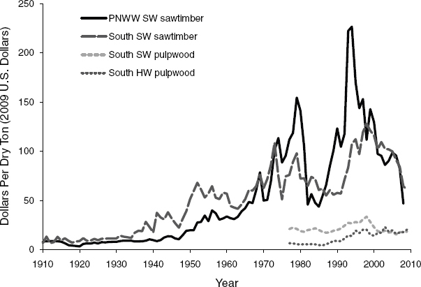
NOTE: Prices are real prices deflated by the all-product producer price index (1982=100). The stumpage price is the value of wood standing in the forest before it is cut.
DATA SOURCES: PNWW SW sawtimber prices from Sohngen and Haynes (1994), Haynes (2008), and Warren (2010); Southern SW sawtimber from Haynes (2008) and Timber-Mart South (2010); Southern SW and HW pulpwood prices from Timber-Mart South (2010).
on private and then on public land in the Pacific Northwest. Nevertheless, given the long time lags between planting trees and harvesting them, continuing changes in the types of products demanded, technological change, and competition with international supplies, it has proven difficult to fully balance supply (for example, investments) and demand in wood resources in the United States over time. Despite the long-term trend upward, timber prices have fallen substantially since their highs in the 1990s and early 2000s.
Current Market for Wood as Energy
In recent years, up to 132 million dry tons (250 million m3) of roundwood equivalent18 have been used to produce energy, though as electricity, not transportation fuel (Figure 4-17). This includes industrial roundwood used directly to produce energy as well as residues, black liquor from the pulping process, and fuelwood harvested from the forest. Industrial energy users in Figure 4-17 are mostly pulp mills and other large integrated wood
______________
18 For definitions of wood products, please see Appendix D.
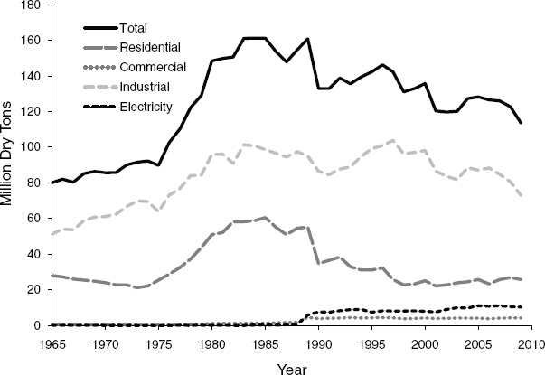
FIGURE 4-17 Wood used in energy.
NOTE: Conversion from Btus assumes 1 Quadrillion Btus = 4 billion ft3, following Howard (2007).
SOURCE: EIA (2010b).
producers that have boilers installed to use residues from the milling or pulping process. These sources of demand for wood were fairly steady from the 1980s to recently. They have declined as overall output in the wood products industry has declined. Wood used in electricity has increased in recent years as energy companies have cofired wood with coal to reduce emissions for air-quality regulations and as additional states have implemented Renewable Portfolio Standards that allow wood to be used for renewable electricity.
Residential wood use for energy initially declined after peaking in the early 1980s but has recently increased. For the most part, residential wood use is in the form of firewood for home heating. Recently, homeowners have increasingly been using wood pellets in wood-burning stoves, and pellets have been used in some industrial processes. Spelter and Toth (2009) estimated that there are about 850,000 heating stoves in the United States and that these and other sources demand more than 2.3 million dry tons of heating pellets. At the time of the publication of this report, pellets were made mostly from sawdust and other residue from milling of lumber and production of plywood. Between 1998 and 2006, the total quantity of sawdust and other residues used in industrial wood production was about 13 million dry tons, and the total supply was about 20 million dry tons. This gap, however, has narrowed in recent years as the supply of residues in the United States has fallen with the decline in wood manufacturing.
Potential Changes Caused by Biofuel Policy
Though many factors beyond biofuel policy affect prices, increased demand for woody biomass due to changes in competition for resources, economic incentives, or technology could have substantial effects on local woody biomass markets and harvesting decisions. Under current conditions, sawtimber is about 3 times more valuable than pulpwood (see Figure 4-16) because of the higher value end-uses it can provide. With any timber harvest, there is a distribution of log sizes. Sawtimber logs typically are the larger logs (more than 7 inches in diameter), and pulpwood logs are the smaller, lower-value logs. Sawtimber products tend to be higher value than pulpwood products and thus are expected to carry higher value. Historically, hardwood pulpwood has been of even lower value than softwood pulpwood, but since the early 2000s, hardwood pulpwood prices have achieved parity with softwood pulpwood as a result of improved technologies for making pulp with hardwoods. Estimates of the value of fuelwood are more difficult to obtain because most of the value lies in the cost of the delivery itself. For example, delivery costs for pulpwood or sawtimber in the southern United States are approximately $35 per dry ton, and fuelwood delivered prices are about $35-$37 per dry ton, according to Delivered Price Benchmark Service from Forest 2 Market, Inc. The difference between the delivery value and the cost of deliver is the stumpage value, which would be about $0-$2 per dry ton. Prices are similar in other parts of the country: for example, New Hampshire reports recent fuel chip stumpage prices of $1-$3 per dry ton (NHDRA, 2010). Pulpwood is the closest marketable commodity that could enter woody biomass markets, and delivered softwood pulpwood prices in the South are substantially higher than fuelwood prices, in the range of $45-$55 per dry ton (Forest2Market, 2010; Timber-Mart South, 2010). These prices represent current conditions. If a commercial woody biomass refinery is built, it would require 1,000-2,000 dry tons of biomass per day to operate efficiently. The competition for resources created by a biorefinery entering the woody biomass market would have profound effects on the local price for woody feedstock.
Economic incentives could raise the profitability of fuelwood and spur additional extraction of residues for market uses, such as cellulosic ethanol production. One way this could be done is by explicitly subsidizing the extraction of residue material (Figure 4-18A). To get a sense for the size of the subsidies necessary, studies in California (Jenkins et al., 2009; Sohngen et al., 2010) found that the cost of removing residues through whole-tree harvesting systems could be as high as $50 per dry ton at the roadside. The costs to deliver 80 or 100 miles (a typical distance for the study site in California by Sohngen et al., 2010) would add $18-$22 per dry ton, suggesting total delivery costs of $72 per dry ton. WTP for this material in California currently is about $30 per dry ton for delivery, suggesting that subsidies would need to be up to $42 per dry ton to induce removals, depending on the region of the country.
A second way in which additional residues may be extracted would be if markets for cellulosic materials began to grow as a result of technological advancement. For example, if the technology for producing cellulosic ethanol improved, then demand for forest-based cellulose would increase from the current low levels, driving up the demand for wood materials in general (assuming that technology does not improve so much that demand for the raw material input falls). This increase in demand for woody biomass in general would influence not only residue recovery but also sawtimber and pulpwood markets. The effect of this increase in demand can be seen in Figure 4-18B, as a shift in the entire demand function. Rising demands for cellulosic materials would have ripple effects through the entire market. Higher values for residues would increase residue collection but would also compete with some lower end pulpwood away from the pulp market. This in turn would
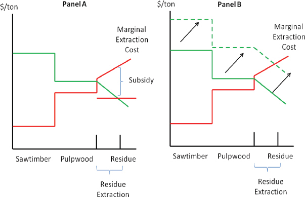
increase pulpwood prices, causing some additional sawtimber at the lower end to be used as pulpwood, which results in higher sawtimber prices. Therefore, though current wood biofuel prices are low compared to pulpwood and sawtimber prices, improving technologies for cellulosic biofuels could raise prices for wood inputs.
The restrictive definition of woody biomass eligible for RFS2 was discussed in Chapters 1 and 2. If technological changes made cellulosic biofuels economically competitive, woody biomass prices could increase because of supply limitations. However, if technologies for cellulosic biofuels do not fully develop and there is no strong demand for cellulosic material, the effects in markets would be modest. In this case, subsidies would be needed to sustain the market (Sedjo, 2010). Figure 4-18, for instance, shows that a subsidy potentially raises the value of the biomass material above the value of pulpwood. Regardless of whether the subsidy is paid to consumers of biomass feedstocks or producers of feedstocks, higher prices for biomass material caused by subsidies could spur conversion of traditional pulpwood supplies to biofuel feedstocks. There is speculation that the initial subsidies in USDA’s Biomass Crop Assistance Program raised the value of pulpwood by subsidizing the use of a wide range of forest materials as bioenergy feedstocks (Box 4-4). Thus, if subsidies are large enough, and not well targeted, they can have unintended consequences and strong implications in markets.
The implications of a demand increase due to RFS2 are large. Sedjo and Sohngen (2009) and Sohngen et al. (2010) used a global timber model to examine a case in which all material needed to produce the cellulosic biofuel mandate would be derived from forests by 2022. Rather than assuming that the material would be derived from residues alone, they assumed that the entire mandate would be derived from existing forest resources within the United
BOX 4-4
Biomass Crop Assistance Program
The Biomass Crop Assistance Program (BCAP) was written into the 2008 farm bill (Section 9001 of the Food, Conservation and Energy Act of 2008 [110 P.L. 234]) as a way to support the establishment of bioenergy crops in selected project areas. The program has two parts. One part provides a subsidy to agricultural producers, individuals, or companies who collect and deliver biomass material to production facilities. The law requires that the biomass is certified to have been collected or harvested with an approved conservation plan. The subsidy amount is $1 per dry ton for every $1 per dry ton paid by production facilities for biomass material, up to a maximum of $45 per dry ton. The payment is limited to 2 years. In an effort to avoid shifting material that already has productive uses into this new “market,” the law defines eligible material for the subsidy restrictively. Eligible material can be forest material from public land that is taken lawfully and does not have a different market use (for example, material from precommercial thinning or invasive plant treatments) or any renewable organic matter from nonfederal land that is not eligible to receive payments from Title I of the farm bill. Animal waste, food waste, yard waste, and algae are not permitted to obtain payments.
The other part of BCAP provides a subsidy for the establishment of biomass energy crops within specific “BCAP Project Areas.” Project areas will be specified by the USDA Farm Services Agency. The payments are for up to 75 percent of the establishment cost and annual payments for up to 5 years for perennial biomass crops and annual payments up to 15 years for woody biomass crops. Most private land qualifies, although land currently in the Conservation Reserve Program (or Wetland or Grassland Reserve Programs) is not permitted to participate.
Between June 2009 and February 2010, enrollment for the part of BCAP that provides payments for collecting, harvesting, storing, and transporting biomass was open and active on a preliminary basis with around $235 million in funding. As of August 2010, these preliminary funds, announced through a Notice of Funds Available, had been spent on around 7.1 million dry tons of material. USDA issued a final rule for BCAP in October 2010.
Many large timber mills registered as BCAP facilities during the enrollment period. Therefore, the bulk of funds has been spent on woody biomass delivered to these facilities. Of the total payments so far, $184 million were spent on woody biomass, $37 million on waste materials, and only about $250,000 on agricultural biomass. Maine, California, Alabama, Georgia, and South Carolina are the top five states, followed closely by Michigan and New Hampshire. With the exception of California, these states tend to be large timber producers and not large crop producers with the types of crops or residues that can be readily harvested for biomass energy. New Hampshire is not a particularly large timber producer, but numerous pellet producers and biomass energy production facilities that use forest inputs for fuel are located there.
To a large extent, the emphasis on the current BCAP payments on forestry activities makes perfect sense, given that forest materials are the most widely available cellulosic bioenergy feedstock. While the technology to convert trees to liquid fuels is costly and not yet commercialized, the technology to convert trees to electricity is available and substantially less costly. Many timber mills already produce electricity with residues from milling operations (including sawdust and black liquor). A number of states now have Renewable Portfolio Standards in place that provide incentives for biomass electricity production. The current data point to the fact that existing boilers using wood for energy have been the largest beneficiary of the subsidies in BCAP so far.
However, there was concern that the subsidy payment for collecting and delivering biomass was creating competition and increasing the price of biomass for other users, such as manufacturers and nurseries. Therefore, it was specified in the final rule that BCAP payments can only be applied to biomass material that cannot be used in higher-value products, such as particle board or composite panels. At the time this report was written, it remained to be seen whether this modification to the payments was implemented effectively (Stubbs, 2010).
Nationally, BCAP subsidies do not appear to have affected timber prices substantially to date. This is largely due to the economic slowdown that has reduced prices for timber in general. Although BCAP is not expected to have substantial effects nationally, some regions could experience important economic effects from increases in fuelwood production. For example, fuelwood stumpage prices have doubled since 2005 in New Hampshire, with the bulk of the increase occurring in 2008 and 2009 as the BCAP program picked up steam (Manomet, 2010).
States (that is, they shift the demand for wood products outward). This is an unlikely scenario in the long run, but it illustrates the potential effects of using only forests to meet the cellulosic biomass mandates. Initially, the cellulosic mandate would use a modest 7.4 million dry tons (14 million m3) of national timber harvest. Given that the United States consumes about 217 million dry tons (410 million m3) per year, this is a small increase. By 2022, however, the cellulosic mandate would use 169 million dry tons (320 million m3) or over 75 percent of the total national timber harvest. Their results indicate that timber prices rise on average by around 5 percent, that U.S. timber production rises by about 7 percent, and that consumption of industrial wood in the United States declines by about 10 percent.
This increase in timber production by 7 percent amounts to only about an additional 15.9 million dry tons (30 million m3) in timber harvests, not nearly enough to match the 169.3 million dry tons (320 million m3) requirement for cellulosic markets. Even though industrial wood consumption declines by 10 percent, or about 21.2 million dry tons (40 million m3), because of higher prices for timber, the United States would have to import additional wood to make up the difference. The model projects that industrial roundwood imports rise 10-fold to meet the timber shortage in the United States caused by the cellulosic biofuel standard.
The Sub-Regional Timber Supply model (SRTS) has also been applied to examine the effects of expanding demand for biomass energy from forest resources in the South (for example, Galik et al., 2009). The SRTS model has substantially more detail than the study by Sedjo and Sohngen (2009) described above and clearly delineates forest residues from other materials; however, the model has not been used explicitly to model cellulosic biofuels. The results for expansion in demand for biomass energy illustrate the implications of rising demand for forest resources.
The specific example considered with the SRTS model is the renewable portfolio standard in North Carolina, which requires 12.5 percent of electricity to be produced with renewable sources, including forests, by 2022 (see Galik et al., 2009). SRTS was used to examine the potential for forest materials, including residues from logging and milling, pulpwood substitution, and new investments in timber resources to be used to meet the renewable portfolio standards.
The authors modeled timber demand and supply in a three-state region, given that supply for the North Carolina market is generated from forests in Virginia, North Carolina, and South Carolina. The wood requirements for this renewable portfolio standard would be as much as 9.4 million dry tons per year from this region, which is nearly as much as the 11.8 million dry tons per year harvested for traditional timber uses (for example, sawtimber and pulpwood). The SRTS model finds that only about 3.5 million dry tons per year (or 38 percent of the total) of this supply could be met with residuals. The rest would have to be met with substitution from other products, higher prices for other products, and increased timber harvesting in the region.
Market Effects Beyond Biofuels
As with food prices, biofuel policy is a complicating factor but not the only force influencing the price of wood products. One example to this effect is the large impact of the economic slowdown in the late 2000s on timber prices in the United States. Although forest output rose globally, timber output fell substantially within the United States (Figure 4-19). The decline in output largely resulted from the precipitous slowdown in housing starts that began in 2006 (U.S. Census Bureau, 2010). After hitting over 2 million in 2005, housing starts fell below 600,000 in 2009. Pulpwood and plywood production also fell, but reductions in these outputs were not as dramatic as lumber output.
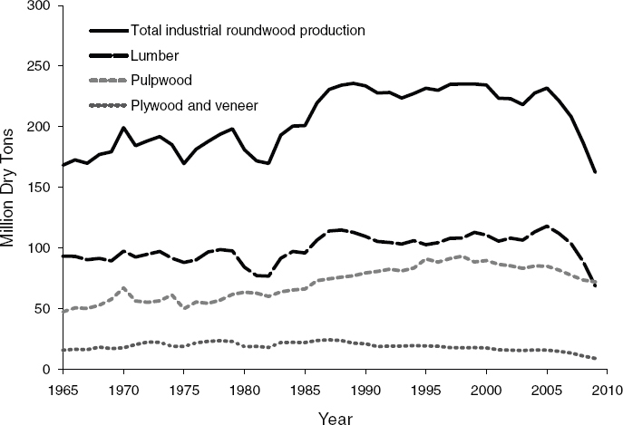
FIGURE 4-19 Industrial wood output in the United States.
SOURCE: Howard (2007); updated data to 2009 as a result of personal communication.
Historically, the United States has been a net importer of industrial wood (Figure 4-20), with about 30 percent of total industrial wood consumption being satisfied by imports in recent years (Howard, 2007). By far, the largest trading partner for the United States is Canada, which provides about 85 percent of total wood imports (Howard, 2007). Imports from Canada grew dramatically after 1990 as output from federal forests in the Pacific Northwest declined, and the closest substitutes in construction were found in Canadian wood (Haynes, 2003). Although Canada is the largest wood products trading partner, the United States is increasingly importing wood from South America. Since 1989, pulpwood imports from South America have risen by about 7 percent per year (USITC, 2010b).
Fossil Fuels
EPA (2010) projected that achieving RFS2 in 2022 will reduce oil imports by 0.9 million barrels per day, a 9.5-percent reduction. Because the United States is the largest consumer of oil, this reduction in demand will lower the world price of oil. According to EPA’s model, meeting RFS2 could decrease the price of oil by $1.05 per barrel in 2022 (EPA, 2010).
USDA’s Economic Research Service (ERS) has also analyzed the effects of introducing 36 billion gallons of biofuels into the transportation economy. It modeled scenarios in 2022 with $80 per barrel oil and $101 per barrel oil. ERS’s results found that, for either price, achieving RFS2 in 2022 would reduce crude oil import prices by about 4 percent, gasoline
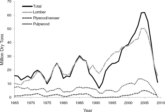
FIGURE 4-20 Net imports of wood into the United States (imports – exports).
SOURCE: Howard (2007); updated data to 2009 as a result of personal communication.
prices by about 8 percent, and the price of motor fuels (gasoline blended with ethanol) by about 12 percent (Gehlhar et al., 2010).
Land Prices
What does the RFS2 mandate mean for land prices? Nearly all the implications of the mandate indicate that land prices will be driven upward. One direct demand factor results from a potential increase in land used for dedicated biofuel crops. For example, if the United States produces 16 billion gallons of cellulosic biofuels by 2022, 30-60 million acres of land might be required for cellulosic biomass feedstock production from forests, pastures, croplands, land from the Conservation Reserve Program, and cropland pasture (land that was once in crops but is not in crops currently) (see Table 4-3). An indirect effect would result from biofuels produced from crop residues because new demand for surplus residue would increase the overall value of land. Thus, although the use of crop residues could reduce that amount of land needed directly for cellulosic feedstock production, the RFS2 mandate still would increase the overall demand for land.
Although it is clear that RFS2 will increase the demand for land and will raise land prices, the exact extent of the effect has not yet been estimated. The use of marginal agricultural land for dedicated bioenergy crops has been proposed as a mechanism to alleviate competition for cropland. Cai et al. (2011) defined marginal agricultural land as land that
has “low inherent productivity for agriculture, is susceptible to degradation, and is high risk for agricultural production.” Based on this definition, they estimated that about 168 million acres of marginal land are available in the United States. However, the availability of marginal land does not imply that bioenergy crops would be grown on those lands. Swinton et al. (2011) analyzed the increase in crop-planted area during the 2006 to 2009 spike in field crop prices. They found that despite an attendant gain in typical profitability of 64 percent, the area of crop-planted area only increased by 2 percent. Even if the profitability doubles, the area of crop-planted area was projected to increase by 3.2 percent, which is about 7.4-10 million acres. Swinton et al. (2011) reasoned that if farmers are reluctant to expand crop-planted area with familiar crops in the short run, they will even be less likely to expand crop-planted area with less familiar perennial dedicated bioenergy crops, which require longer time for crops to establish than annuals. Given the price gap between WTA and WTP for cellulosic biomass, it seems even less likely that farmers would be willing to expand crop-planted area to grow dedicated bioenergy crops. (See also section “Social Barriers” in Chapter 6.) The size of the increase will differ depending on land and crop productivity, other land uses in the region, and the growth of the biofuel sector locally.
EFFECTS OF BIOFUEL PRODUCTION ON THE BALANCE OF TRADE
Effect on Import and Export of Grains
To the extent that biofuel production leads to or has led to increases in the price of corn and other agricultural commodities, the quantity of these commodities exported could be expected to decrease to the extent that export quantity demanded responded to the higher price. The United States is a major exporter of corn, wheat, and soybeans, as well as some animal products. Higher crop prices eventually would lead to higher livestock product prices and reductions in exports of those products. Since 2002, however, while crop commodity prices were rising, exports of many of these commodities held steady or even increased (see Figure 4-13). The main reason for this occurrence is the huge depreciation in the U.S. dollar between 2002 and 2008. With a lower value for the U.S. dollar, commodity prices did not increase nearly so much in other currencies such as the euro or yen. Therefore, exports were not as affected as would have been expected in the absence of the depreciation in the U.S. dollar.
Livestock Production and Trade
Increased animal product costs as a result of the simultaneous implementation of RFS2 and EU biofuel mandates are expected to decrease the global value of livestock industries by about $3.7 billion (2006$) cumulatively between 2006 and 2015 (Taheripour et al., 2010). Most of this decrease would occur outside the United States, which would observe only a minor reduction ($0.9 billion) in its livestock and processed livestock products. The effect in the United States is buffered by the increasing availability of coproducts from corn-grain ethanol production, especially DDGS (see earlier section “Ethanol Coproducts”). Changes in livestock production are not predicted to occur evenly across species. Ruminants are better adapted to use DDGS than nonruminants and would be affected less. This is reflected in an expected increase in the trade balance for ruminant products of $135 million but a decrease for nonruminant products of $40 million (in 2006$) (Taheripour et al., 2010).
Effect on Import and Export of Wood Products and Woody Biomass
As discussed earlier (see section “Wood Products”), the United States imports a large quantity (over 30 percent) of its wood resources from outside the country (Howard, 2007). Most imports come from Canada, but in recent years, other countries have increased their exports of wood products to the United States. Although the United States is a net importer of wood, it exports some products. One example is wood pellets, which are currently made most often from sawdust obtained from milling operations. This market is relatively small at present but is growing and could continue expanding if demand remains strong in other countries that use pellets for industrial heating (Spelter and Toth, 2009).
Current estimates suggest that the RFS2 mandate would likely increase wood imports into the United States. Wood is the most widely available cellulosic bioenergy feedstock in the United States at present, and it will be an important source of supply for cellulosic biofuel refineries as RFS2 is implemented in the next 11 years. Sedjo and Sohngen (2009) suggested that up to 75 percent of wood currently used by wood producers could shift into biofuel production if the RFS2 mandate pushes supply prices high enough. A shift in industrial wood from traditional uses to biofuels in turn would cause the United States to import more industrial wood from elsewhere. The scale of this effect, however, cannot be precisely estimated at this time.
Effect on Import and Export of Petroleum
Between 2010 and 2022, imports of crude oil are projected to decline slightly, due in part to increased fuel efficiency standards in vehicles and to the RFS2 mandate. As mentioned earlier, EPA (2010) projected that achieving RFS2 in 2022 will reduce oil imports by 0.9 million barrels per day, a 9.5-percent reduction that would save $41.5 billion that year. EPA also estimated that 2 billion gallons of ethanol will be imported to meet RFS2; therefore, the estimated net savings would be $37.2 billion (2010).
BUDGET, WELFARE, AND SOCIAL VALUE EFFECTS OF RFS2
Government policies that support biofuels interact with each other and other federal subsidy programs, particularly those involving farming, conservation, and nutrition. Because they involve tax credits and tariffs, these policies also affect federal government revenue. Government programs are shaped, in part, by public opinion of the value of biofuels, particularly as they pertain to the environment.
Distribution of Benefits and Costs
An economic analysis of the U.S. biofuel policy must consider the three elements that support that policy: (a) the consumption mandate requiring the use of biofuels as an input in the production of transportation fuels, (b) the federal tax credit for biofuels used in the production of transportation fuels, and (c) the import tariff on ethanol used in the production of transportation fuels. This section considers the likely welfare consequences of each of the three elements both in isolation and in combination with the other two.
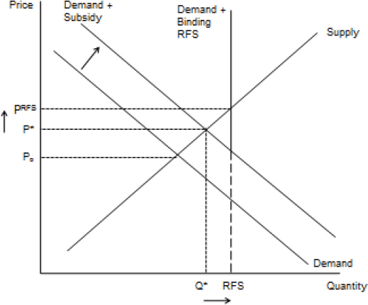
NOTE: PO = price of biofuel without tax credit; P* = price of biofuel with tax credit; Q* = quantity of biofuel with tax credit; RFS = mandate quantity; PRFS = price with tax credit and RFS2 mandate.
Consumption Mandate
The consumption mandate for RFS2 is described in Chapter 1 (see section on “Renewable Fuel Standard”). Under a consumption mandate, if the price of renewable biofuel is greater than the price of gasoline, the mandate would have the effect of raising the price of transportation fuels. Such an increased input cost would cause an increase in the cost of transportation fuels and a kink in the biofuel demand curve as shown in Figure 4-21. In essence, the biofuel demand curve becomes totally insensitive (inelastic) to the biofuel price because that level of consumption is required by the mandate. The higher price of biofuel as a result of the mandate would lead to a higher price of blended fuel and, consequently, reduced blended fuel consumption because of this higher price. Because the price elasticity of demand for transportation fuels is inelastic, the reduction in consumption would be small. Thus, the consumption mandate would result in the following effects, assuming no changes in technology, vehicle fuel-use efficiency, use of flex-fuel vehicles, and transportation fuel infrastructure:
1. With an increase in the price and a decrease in the quantity of transportation fuels consumed, the welfare of fuel consumers will decrease;
2. With an increase in the price and a decrease in the quantity of transportation fuels consumed, the welfare of biofuel producers will increase;19
3. With an increase in the quantity of biofuel demanded, the demand for biofuel feedstock will increase;
4. With an increase in the price and quantity of biofuel feedstock demanded, the welfare of feedstock producers will increase;
5. With an increase in the price and quantity of feedstock demanded, the demand for resources used to produce feedstock (for example, land, labor) will increase;
6. With the increase in the demand for resources used to produce feedstock, an increase in the price and quantity of resources used will increase the welfare of owners of resources used in the production of feedstock (for example, landowners);
7. With the increase in the price of resources used to produce feedstock, competing users of those resources will pay a higher price to retain those resources and the quantity of those resources used for production of other products will decrease;
8. As the quantity of resources used in the production of feedstock increases, the quantity of those resources used in the production of other goods (for example, food, livestock feed) decreases;
9. As the quantity of resources used in the production of other goods decreases, the quantity supplied of these other goods will decrease and their prices will increase;
10. As the price of these other goods increases and the quantity decreases, the welfare of consumers of these goods will decrease and the change in the welfare of producers of these goods will be determined by the price elasticity of demand for these goods; and
11. Though the mandate has no direct effect on federal government expenditures, the indirect effects could include:
a. To the extent that RFS2 increases the prices of agricultural commodities that receive commodity program support payments, the size and cost of those payments will decrease;
b. To the extent that RFS2 increases the prices of agricultural commodities and, therefore, the price of food and expenditures for those federal programs whose payments are related to the food price level (that is, expenditures that are increased to reflect the Consumer Price Index such as the Supplemental Nutrition Assurance Program [SNAP], the Special Supplemental Assistance Program for Women, Infants, and Children [WIC], or Social Security programs) will increase.
Tax Credit for Blended Biofuels
A second policy tool to support biofuels is the tax credit provided to blenders for using biofuels. As discussed in Chapter 1, tax credits exist to encourage the blending of corn-grain ethanol, biodiesel, and cellulosic biofuel into transportation fuel. Because the credit for corn-grain ethanol has been in place the longest and much more corn-grain ethanol has been consumed in the U.S. transportation market, this section will focus on the economic effect of the tax credit for corn-grain ethanol.
______________
19 The effect on the welfare of transportation fuel producers will depend upon the price elasticity of the demand for fuel. If the price elasticity of demand for fuel is inelastic, the percentage increase in price will be greater than the percentage decrease in quantity. Thus, the welfare of fuel producers will increase. Most studies of the price elasticity of demand for fuel have concluded that the demand for fuel is inelastic with regard to price (Espey, 1996, 1998; Graham and Glaister, 2002; Goodwin et al., 2004).
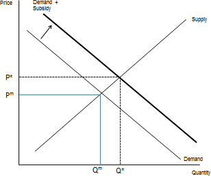
FIGURE 4-22 Effect of the Volumetric Ethanol Excise Tax Credit on price and quantity of ethanol.
NOTE: Pm = market price of ethanol without tax credit; P* = market price of ethanol with tax credit; Qm = quantity of ethanol without tax credit; Q* = quantity of ethanol with tax credit.
Under the legislation in action when this report was written, fuel blenders received a tax credit of $0.45 per gallon of corn-grain ethanol blended with gasoline, known as the Volumetric Ethanol Excise Tax Credit (VEETC). As illustrated in Figure 4-22, the effect of VEETC is to shift the demand for biofuel up and to the right because the blender is willing to pay more for every gallon of ethanol that receives the tax credit. In Figure 4-22, Pm and Qm are the market price and quantity without the tax credit and P* and Q* those values with the tax credit.
The demand curve for ethanol is derived from the demand for gasoline transportation fuel. Therefore, the impact of the tax credit is to increase the price of ethanol and the quantity of ethanol produced relative to the absence of the tax credit. The impact on consumers is difficult to predict as the tax credit would be shifted among the blender, biofuel producer, and consumer depending on market supply and demand conditions.
This increased use of ethanol would result in an increase in the demand for biofuel feedstock, as noted in item 3 in the list of effects in the previous section. Following this change in the market for biofuel feedstock, the welfare consequences of a tax exemption would be identical to those noted in items 4 to 10 of the previous section, given no other changes.20 For item 11 (the effect on the budget of the federal government), however, the
______________
20 The size of these welfare changes, however, would depend on the relative size of the change in biofuel consumption caused by the mandate versus the tax exemption.
tax credit policy would also result in the loss of federal tax revenue equal to the volume of gasoline displaced by biofuel multiplied by the VEETC ($0.45 per gallon) (see “Federal Fuel Tax Revenue” below). Thus, this results in either less funding available for government projects or higher taxes elsewhere to compensate for the shortfall in revenue.
Import Tariff
The third policy instrument to support the production and use of domestic biofuels is a tariff on imported ethanol. The current tariff is $0.54 per gallon plus 2.5 percent of import value; at recent ethanol prices, the total tariff equals about $0.59 per gallon. However, imported ethanol receives the same blender’s tax credit as domestic ethanol ($0.45 per gallon), so the net tariff is about $0.14 per gallon. An import tariff on ethanol (considered in isolation from the consumption mandate and the tax credit) normally causes a decrease in the quantity of ethanol imports. Reduced imports would lead to increased domestic production. Given that imported sugarcane ethanol can be used to fulfill the other advanced biofuels category once that category of RFS2 becomes binding, it is not clear that the tariff at that point would reduce imports substantially.
Policy Interactions
Though the analysis above is indicative of each policy’s effect, the use of these policies in combination can result in consequences that can be similar or, in particular circumstances, offsetting in nature (de Gorter and Just, 2010). If, for example, the consumption mandate policy is used in combination with the import tariff policy, the results of the mandate policy would be identical to those outlined above for the quantity of biofuel used to fulfill the consumption mandate (regardless of the domestic or foreign source of the biofuel).21 However, RFS2 has four categories of biofuels, each with separate GHG rules. If the imports are based on sugarcane, they can be used for the “advanced biofuel” category, which has its own criteria, so the markets would be segregated. Beyond that point, any additional consumption of biofuel would be determined by the price of biofuel (including the import tariff) relative to the price of gasoline. If the price of biofuel (mileage-adjusted) is less than the price of gasoline, then a quantity of biofuel beyond the mandate would be consumed (up to any technical limit or “blend wall”). If the price of biofuel is greater than the price of gasoline, then no biofuel beyond the mandated level would be consumed.
If the import tariff policy is used in combination with the tax credit policy, then the welfare effects identified above would be the same, but the size of the anticipated welfare effects would be determined by the relative sizes (on a per gallon basis) of the import tariff and the tax credit. The net effect of these two policies would then determine the price of biofuel and its use as a substitute for gasoline in the production of transportation fuels. As before, if the price of biofuel (on a mileage-adjusted basis) resulting from the net effect of the combined policy is less than the price of gasoline, then the quantity of biofuel used would increase (until reaching any technical limitation).
______________
21 Though the direction of any welfare changes of a combined mandate and tariff policy would be identical to those identified for the mandate policy, the magnitude of the combined policies would likely be greater than those of a consumption mandate policy used in isolation. This result would occur because the combined policy is likely to increase the magnitude of any price changes that occur (i.e., the price of biofuel is likely to be greater under the combined policy). In addition, if the tariff applied to the price of imported biofuel is prohibitive (i.e., the cost of imported biofuel is greater than the cost of domestic biofuel), then a zero quantity of biofuel would be imported and the welfare consequences would be the same as if the consumption mandate had been used in isolation.
A combination of the consumption mandate policy and the tax credit policy can result in a wider variety of consequences. Once the consumption mandate is filled (that is, the quantity of biofuel consumed equals the quantity of biofuel required by the consumption mandate), any additional use of biofuel in the production of transportation fuel will be determined by the relative prices of biofuel and gasoline. If the price of biofuel is less than the price of gasoline, then the quantity of biofuel consumed would be greater than the mandated level. In this case, the welfare effects of a combined policy would be the same as indicated above, but the magnitude of these changes would be larger for a combined policy than for a mandate policy alone. In addition to the welfare effects noted above, a combined policy would also result in a loss of federal fuel tax revenue equal to the quantity of gasoline consumption displaced by biofuel multiplied by the level of the tax credit. In the case of corn-grain ethanol, the Government Accountability Office (2011) found the existence of both policies to be redundant because the infrastructure for the ethanol industry has been developed and no longer needs the additional incentive of the VEETC to create capacity to meet the RFS2 mandate. If, on the other hand, the price of biofuel is greater than the price of gasoline, then no additional biofuel would be consumed beyond the mandated quantity. However, if the cost difference is less that the level of the tax credit, then the blender’s credit could still induce additional biofuel production.
Finally, if all three policies are used in combination, then the welfare effects of the combined policy would be determined by (a) the mandated consumption quantity and (b) the net price effect of the tax credit and the import tariff policy. The import tariff would increase the price of biofuel. The net effect of these two policies would then determine the price of biofuel and its use as a substitute for gasoline in the production of transportation fuel. If the price of biofuel (on a mileage-adjusted basis) resulting from the net effect of the combined tax credit and tariff policy is greater than the price of gasoline, then the quantity of biofuel consumed would equal the quantity of biofuel required by the mandate. If the net price of biofuel is less than the taxed price of gasoline, then the quantity consumed would exceed the mandated quantity. All of these projections are based on no other changes in the biofuel system.
State-Level Policies
In addition to the federal-level policies affecting biofuel consumption and production, state government policies also affect the biofuel market. These policies include a varying combination of incentives (construction grants, capital cost subsidies, tax incentives, loans and leases, rebates, exemptions) and regulations that influence the consumption of biofuel (mandates, air quality, carbon intensity, climate change initiatives). Because such policies vary widely across states, it is difficult to determine the level of subsidy or mandate that would be created by these state-level policies when considering their effects on a nationwide basis (Tyner, 2008). Comparing the magnitudes of federal and state policies, however, suggests that the welfare effects of federal policies are of greater magnitude than state-level policies (Box 4-5) (Steenblik, 2007; Koplow, 2009). For example, state tax credits often are in the range of $0.20 per gallon but can be as high as $1.00 per gallon (Kentucky). At the same time, state subsidies “add substantially to the profitability of production from existing facilities [but] they are often provided up to an annual limit” (Steenblik, 2007, p. 25). In some states, mandates or tax credits are contingent on the use of feedstock produced in the same state (Steenblik, 2007). Local levels of government sometimes provide production subsidies in the form of property tax abatements, economic development loans, infrastructure subsidies, or free use of land (Steenblik, 2007). In addition, such state-level policies are likely to
BOX 4-5
State and Federal Subsidy Expenditures on Energy in Texas
In 2008, the Comptroller of the State of Texas produced an extensive report examining the existing and potential resources Texas can employ to meet its energy demands (TCPA, 2008). This report included a chapter on the subsidies that various energy sources received in 2006, the last year with complete data when the report was being prepared.
According to the report, governments provide subsidies in the form of tax incentives (such as depletion allowances, accelerated depreciation, and reductions in excise taxes), direct spending for government services, the assumption of certain types of liability or risk by the government, government ownership of energy production, access to resources on government land, and tariffs.
The report breaks down the subsidies into two categories, those coming from the federal government and those coming from the State of Texas. Texas is a large consumer and producer of energy of many kinds. As such, its support of various energy industries through incentives for increased production is probably higher than most states. The state subsidies are for the energy used in Texas alone. Table 4-5 shows federal and state subsidies for various energy types as a percent of total consumer spending for the sources.
TABLE 4-5 Energy Subsidies as Percentage of Consumer Spending on That Source
| Energy Source | Federal Subsidies | Texas Subsidies |
| Oil and Gas | 0.5 | 1.5 |
| Coal | 6.9 | 0 |
| Nuclear | 20.9 | 0 |
| Ethanol | 26.5 | 0 |
| Biodiesel | 9.9 | 3.1 |
| Wind | 11.6 | 0.2 |
| Solar | 12.3 | 9.2 |
| Other Renewable | 0.5 | <0.1 |
SOURCE: TCPA (2008).
Total federal subsidies for corn-grain ethanol and biodiesel sold in 2006 were $4.71 billion and $92 million on 4.8 billion gallons of ethanol and 250 million gallons of biodiesel. These subsidies totaled $0.98 per gallon for ethanol and $0.38 per gallon for biodiesel.
Substituting corn-grain ethanol or biodiesel, the only current alternatives for liquid transportation fuel for gasoline and diesel, will have a substantial effect on government tax revenues. RFS2 requires the inclusion of an additional approximately 20 to 25 billion gallons per year of biofuels in the transportation fuels sold in the United States by 2022. With the current tax structure, this would reduce state and federal excise tax revenues by over $10 billion per year.
have their greatest effect on the location of biofuel refineries among states rather than the total national biofuel production capacity (Cotti and Skidmore, 2010).
Federal Budget Effects
The net effect of RFS2 on the federal budget would be determined by changes in the following:
- The cost of farm commodity program payments;
- The cost of other USDA programs, including conservation programs;
- The cost of nutrition and income transfer programs that are affected by changes in the price of food through the CPI;
- The cost of biofuel production subsidy programs;
- The federal fuel tax revenue forgone due to tax credits, in particular the VEETC for corn-grain ethanol; and
- The tariff revenue generated or forgone by the tariff on imported ethanol.
Though these budget changes can be difficult to estimate with precision, the provisions of RFS2, the tax credits, and the import tariff and past experience with biofuel production can suggest the direction and general magnitude of the changes that would occur for each budget component.
Agricultural Commodity Programs
An increase in biofuel production encouraged by the RFS2 mandate can indirectly produce savings in federal payment programs that support agricultural commodities; however, the circumstances under which such savings are realized is rather specific and limited. Under the Food, Conservation, and Energy Act of 2008, commodity support programs consist of a direct payment program, a countercyclical payment program, and a marketing assistance loan or equivalent loan deficiency program.22 To determine the effect of RFS2 on the budget cost of these programs, each program is considered. The first type of payments—direct payments—are fixed payments provided to crop producers regardless of the market price received by crop producers. As noted earlier, if an increase in the production of biofuel feedstocks results in an increase in competition for those resources (for example, land) that produce other crops, the prices of those other crops would be expected to increase. This increase in crop prices would not affect the budget cost of the direct payment program, however, because direct payments are paid to crop producers regardless of the price level. Thus, under no circumstances would meeting the RFS2 mandate generate savings in the budget cost of the direct payment program.
The second type of payments—countercyclical payments—are paid when the market price for a crop is less than the effective target price of that crop. The effective target price of a crop is calculated as the legislated target price of that crop minus the direct payment of that crop. For example, under the Food, Conservation, and Energy Act of 2008, the target price for corn is $2.63 per bushel and the direct payment for corn is $0.28 per bushel in the 2012 crop year. The effective target price for the 2012 crop year will be $2.35. If the market price, without the implementation of RFS2, is $2.35 per bushel or more, the budget savings of RFS2 will be zero (that is, no countercyclical payment would be made because the market price is greater than the effective target price even without the price effect of RFS2). Thus, only if the market price would be less than $2.35 without the implementation of RFS2, and then increases to above $2.35 with RFS2, can any budget savings in the countercyclical payment program be realized. Similarly, the marketing assistance loan program establishes a marketing loan rate of $1.95 per bushel in 2012. If the market price of corn is less than $1.95, corn producers would be eligible for a loan deficiency payment equal to the difference between the marketing loan rate and the market price. Thus, only if the market price would
______________
22 Crops included in these programs include corn, wheat, soybean, rice, cotton, peanuts, grain sorghum, barley, oats, and other oilseeds. The Food, Conservation, and Energy Act also established the Average Crop Revenue Election program (ACRE) as an alternative to the Direct and Countercyclical Payment program (DCP). Since a large majority of commodity producers have chosen to remain enrolled in the DCP program, this analysis will examine the budget consequences of biofuel production on the budget cost of the DCP program.
be less than $1.95 without the implementation of RFS2, and then increases to above $1.95 with RFS2, can any budget savings in the marketing loan assistance program be realized.23
Long-term projections of U.S. agricultural commodity prices from 2011 to 2021 suggest that market prices will exceed effective target prices during that period. For example, USDA projections of corn (ranging from $4.10 to $5.20), soybean ($10.25 to $11.45), and wheat prices ($5.45 to $6.50) would exceed the existing effective target prices during the period (USDA, 2011). If such projections hold true, then the change in the budget cost of commodity programs attributable to an expansion of biofuel production (which presumably would result in price levels higher than these levels) would be zero because market prices would exceed effective target prices (thus, no countercyclical payments would be made) and direct payments would be unchanged (paid regardless of market price levels). Similarly, long-term price projections from the Food and Agricultural Policy Research Institute (FAPRI, 2010) also suggest that market prices of these three agricultural commodities would exceed effective target prices during the period, again supporting a conclusion that expanded biofuel production would likely result in no change in the budget cost of commodity programs.24
Conservation Programs
The Conservation Reserve Program (CRP)—a conservation program in which farmers sign contracts with the federal government to take land out of crop production for a period of time for which they receive payment—is the largest federal conservation program directed at agricultural land. Under the 2008 farm bill, CRP is limited to 32 million acres, down from 39.2 million acres under the previous farm bill. Only land that was planted to an agricultural commodity in four of the previous 6 years from 1996 to 2001 or land that is suitable as a riparian buffer is eligible for CRP. Land is typically enrolled for 10-15 years, and, at the time this report was written, participants received an average payment of $44 per acre. In the summer of 2010, 31.3 million acres were enrolled. The program was estimated to cost $1.7 billion in fiscal year 2010, $250 million less than fiscal year 2009 (Cowan, 2010).
The effects of biofuel policy regarding expenditures on CRP are uncertain. Higher commodity prices, to which biofuel may be a contributing factor, could entice growers to remove acres from the program. CRP costs would decrease if further acres were not enrolled to replace acres leaving the program. The likelihood of declining acres is unknown: In the previous two general sign-ups for CRP (2006 and 2010), the number of acres bidding for the program exceeded the number of acres accepted (Cowan, 2010). However, if acres left the program and were not replaced by other enrollments and if keeping maximum enrollment is an important objective of CRP, then payment rates would have to increase to compete with commodity prices. Likewise, competitive CRP payment rates could incentivize producers to keep the most sensitive land in the program. This action could increase
______________
23 Thus, if the market price is below $1.95, a corn producer would be eligible for a target price of $2.63 that would consist of the market price (below the loan rate of $1.95) plus the loan deficiency payment (equal to $1.95 minus the market price) plus the countercyclical payment (equal to $2.35 minus the loan rate of $1.95) plus the direct payment ($0.28), thereby providing the target price of $2.63.
24 The assumptions regarding biofuel production policies used in each of these studies should be noted. USDA assumes that all tariff and tax credit policies for ethanol will remain in place for the entire 2011-2021 period. Similarly, the FAPRI projections incorporate the mandates contained in EISA but assume the mandate regarding use of cellulosic ethanol is waived (i.e., only the EISA mandate of 15 billion gallons of conventional ethanol is continued) and that all tariffs and tax credits for biofuels are extended for the entire period.
the cost of the program, depending on the new payment rate and the number of acres that remain in CRP.
Harvest and grazing are allowed on CRP land under certain conditions. For example, if the government has defined a drought as a disaster, the harvesting of hay or grazing of cattle may be permitted under the 2008 farm bill. Routine harvesting may also be allowed to manage invasive species (Cowan, 2010). It has been suggested that bioenergy feedstocks could be cultivated on CRP land as long as certain criteria were met, such as requiring the harvest to occur after the bird-nesting season. CRP payments would be reduced in accordance with the revenue generated from harvesting biomass. With appropriate environmental restrictions, such compromise would allow conservation and biomass production to coexist while also reducing government CRP payments. However, an attempt in 2008 to classify some CRP land as eligible for haying and grazing for animal feed purposes was suspended by a lawsuit requesting further environmental review, and similar authorization was not made in 2009 or 2010 (Cowan, 2010). At the time this report was written, it appeared unlikely that cultivating biomass would be permissible on CRP land.
Nutrition and Income Transfer Programs
As noted earlier (see “Food Prices”), assessment of any change in food prices resulting from expanded biofuel production would have to consider the effect on agricultural commodity prices and the transmission of that commodity price effect through the food system to the retail level. Similarly, those two factors have to be considered in assessing the effect of an expansion of biofuel production on the budget cost of nutrition and income transfer programs. The experience of the 2007-2009 period provides useful examples for understanding the likely impact of expanded biofuel production under RFS2.
Nutrition and other income assistance programs are often adjusted for changes in the general price level as a means of protecting the real purchasing power of program recipients. This adjustment is based on the annual change in the CPI. If an increase in the production of biofuel feedstocks results in increased competition for resources (such as land) used to produce agricultural commodities for food, crop prices would be expected to increase, thereby increasing food prices and the food component of the CPI. In turn, the budget cost of those programs tied to the CPI would increase. For example, two programs would be affected by changes in food prices—SNAP and WIC. As discussed earlier (see section “Primary Market and Production Effects of U.S. Biofuel Policy” in this chapter), the role of biofuels in the increase in commodity prices is extensively debated in the literature. The Congressional Budget Office (2009) conducted a study that examined the effect of corn-grain ethanol use on food retail prices and GHG emissions between April 2007 and April 2008. It assumed that 10-15 percent of the increase resulted from biofuels. This translated to an increase in annual expenditures on SNAP of $500 to $800 million and less than $75 million on WIC in the 2009 fiscal year.
To the extent that ethanol production is now a permanent part of the commodity market through the RFS2 mandate, these increases could become a permanent increase in the annual cost of these programs. At the same time, because other programs are also adjusted according to changes in the CPI, these estimates are likely to be lower-end estimates of past and future budget costs for such programs. For example, programs such as Social Security, military or civilian retirement programs, and Supplemental Security Income are adjusted for changes in the CPI, while such items as food purchases for military personnel are affected directly by the prices of food purchased. The budget cost of such programs, and thus the increase in the budget cost of these programs attributed to expanded biofuel
production, would likely dwarf the estimated budget costs of the SNAP or WIC programs. For example, the SNAP program had a projected total budget cost of $54.4 billion in 2009. This compares to an annual budget cost of Social Security and Supplemental Security Income payments of $709.6 billion in 2009 (OMB, 2010). These programs are also adjusted by changes in the CPI to protect the real purchasing power of program recipients. Thus, any calculation of the effect of expanded biofuel production on budget cost of Social Security and other federal programs would likely be much larger than the estimated cost for the SNAP program or other similar programs. However, an increase in raw commodity prices such as corn translates into a much smaller increase in food prices (see earlier section “Food Prices” in this chapter).
These estimates suggest the likely direction and magnitude of changes in budget costs that would be observed with an increase in biofuel production under RFS2. The primary effect on budget costs for nutrition and income transfer programs would be through the increase in retail food prices that would be related to a possible increase in competition for production resources (such as land) resulting from increased production of biofuel feedstock. In particular, the production of crops dedicated to cellulosic biofuel production could result in increased agricultural commodity prices if the production of those crops displaces production of crops devoted to food. For those crops that could be used for both food (for example, corn for grain) and for cellulosic feedstock (for example, corn stover), such joint products could compete more favorably for production resources at the farm level. For example, in the case of corn, producers might find it profitable to continue corn production for food, corn-grain ethanol, and cellulosic biofuel, rather than producing a crop devoted only to biofuel production. In such a case, the shift of acreage from food crops to crops devoted only to biofuel might be limited. Therefore, the effect of expanded biofuel production on agricultural commodity production and on retail food prices could be small.
Federal Fuel Tax Revenue
Another effect of expanded biofuel production on the federal budget is through the federal tax credits for biofuels blended with motor fuel. An estimate of the revenue forgone by the federal government is determined by the size of the federal tax credit provided to blenders of biofuels, the energy equivalence of biofuels and gasoline, and the quantity of biofuel receiving the tax credit (CBO, 2010). The federal tax credit for corn-grain ethanol, the VEETC, has had a nominal value of $0.45 per gallon since 2005. Considering all of the factors noted above, however, this tax credit by some calculations has had a gasoline-equivalent value of $1.78 per gallon in forgone revenue for the federal gasoline excise tax (CBO, 2010). The federal tax credit for ethanol is estimated to be a tax expenditure (that is, forgone revenue for the federal gasoline excise tax) of about $2.9 billion in the 2007 fiscal year, compared to $921 million in 1999 (EIA, 2008b). GAO (2011) found that the VEETC resulted in $5.4 billion in forgone revenue in 2010, which would grow to $6.75 billion in 2015 with increased ethanol production (GAO, 2011).
Because the monetary cost of cellulosic biofuel and other advanced biofuel is expected to be substantially greater than the cost of corn-grain ethanol, the nominal value of the federal tax credit is $1.01 for cellulosic biofuel. When all of the factors noted above are included, however, the cost of this tax credit, in terms of federal gasoline excise tax revenue forgone, could be $3.00 per gallon of cellulosic biofuel (CBO, 2010).
Import Tariff Revenue
The impact of expanded biofuel production on changes in tariff revenue also would affect the federal budget. The potential budget effects of a tariff on ethanol imports depends on the tariff rate charged on imports of ethanol and the quantity of ethanol imports. The effect of these trade restrictions will be determined by the “restrictiveness” of the trade restraint (or “size” of the import tariff) and the responsiveness of market participants (producers and consumers of ethanol in both domestic and foreign markets) to changes in market prices (USITC, 2009).25
As noted above, the tariff on imported ethanol has two parts—the 2.5 percent tariff on all ethanol, and the $0.54 per gallon duty on all ethanol imported for use as transportation fuel. Since the $0.54 per gallon duty is the only portion of the restriction applied specifically to ethanol used as transportation fuel, this analysis considers only this portion in analyzing the tariff revenue from ethanol imports. Under two circumstances, the revenue generated by a tariff can be equal to zero or very near zero.
On the one extreme, a tariff can be so small that the revenue generated by the tariff is near zero. In this case, the tariff multiplied by the value or quantity of the good imported is near zero because the tariff is near zero. At the other extreme, a tariff can be so large that it is prohibitive for exporters of the good. In other words, when the tariff is applied to the value or price of the good, the cost of the imported good exceeds the cost of domestically produced goods. Thus, the quantity of the good imported is now zero (or near zero), so the tariff revenue will equal zero (the large tariff multiplied by a zero quantity imported will equal zero tariff revenue). This issue is particularly important when considering the import tariff on ethanol used as transportation fuel. On the one hand, the general tariff of 2.5 percent on all ethanol is near zero. Thus, the revenue generated by this general tariff would be nearly zero. On the other hand, the $0.54 per gallon duty on ethanol is nearly prohibitive at present on imports of ethanol for transportation fuel. Thus, the tariff revenue generated by this duty also is close to zero. The removal of the $0.54 import duty on ethanol, while leaving the 2.5 percent tariff in place, would move the market from one extreme to the other. That is, the tariff revenue generated by the $0.54 duty would be nearly zero because the imported quantity is nearly zero. If that duty is removed, the tariff revenue generated after that duty is removed would again be zero because the remaining 2.5 percent general tariff is near zero while the quantity imported would likely increase.
Analysis of the effect of removing the $0.54 duty on corn-grain ethanol after the Renewable Fuel Standard under the Energy Policy Act of 2005 went into effect but before RFS2 under EISA was enacted suggests that more ethanol would be imported (USITC, 2009). This analysis found that elimination of the duty would reduce the price of imported ethanol by 25 percent and increase the value of imports by 205 percent annually. This increase in imports would reduce domestic production of ethanol by 2 percent below the level produced under the $0.54 duty (USITC, 2009).26
______________
25 In particular, the change in imports resulting from a removal of trade restraints (tariffs) is likely to be determined by (a) the elasticity of substitution between imported and domestic goods, measuring the ability of users to substitute imported goods for domestic goods, (b) elasticity of import supply, measuring the responsiveness of domestic producers and consumers to changes in the price of that good, (c) elasticity of export demand, measuring the responsiveness of foreign producers and consumers to changes in the price of that good, (d) elasticity of substitution between inputs in production, measuring the ability of domestic and foreign producers of that good to substitute alternative inputs in the production of that good, and (e) income elasticity of domestic and foreign consumers, measuring the responsiveness of consumer demand to changes in consumer income (USITC, 2010a).
26 The value of corn production would decrease by 0.6 percent and the value of corn exports would increase by 0.6 percent annually with the removal of the $0.54 duty (USITC, 2009).
Other Federal Programs Related to Biofuel Production
An additional category of budget costs related to RFS2 is that set of programs that provide subsidies for the production of cellulosic biofuel. Such subsidies take a variety of forms, and similar programs have been provided for the production of corn-grain ethanol, often on an intermittent basis, since 1980 (Duffield et al., 2008). In recent years, such subsidies have increased as part of the policy objective of increasing biofuel production.
The two largest costs associated with a biorefinery are the capital cost of the refinery facility and the cost of the feedstock processed in the facility (see Figure 4-6). Thus, federal biofuel production subsidies have taken a variety of forms, but most programs are designed to subsidize the production cost of the biofuel refining industry by lowering the capital cost of the construction of biorefinery facilities, reducing the variable cost of biofuel feedstock paid by biofuel refiners, providing implicit subsidies to the purchase price of cellulosic biofuel, or decreasing the total cost of biofuel production through the improvement of biofuel processing technology.
Subsidies to reduce the capital investment cost of constructing cellulosic biofuel refineries are typically provided in the form of tax credits, grants, loans, or loan guarantees that provide a rate of interest below that which investors could obtain from alternative financing sources (Table 4-6). For example, the Food, Conservation, and Energy Act of 2008 and the Energy Policy Act of 2005 included a variety of provisions to subsidize the capital cost of constructing cellulosic biofuel refineries. Some of these programs provided subsidies aimed at refineries using a particular form of biofuel feedstock (for example, municipal solid waste) while others provide capital subsidies for refineries without specifying the form of biofuel feedstock.
The second form of biofuel production subsidies, those that reduce the cost of feedstock purchased by cellulosic biofuel refineries, are typically provided in the form of payments per unit of feedstock purchased (Table 4-6). Such payments reduce the purchase price of biomass feedstock for biofuel refineries and, therefore, the production cost of biofuel products. The payment through BCAP for collecting, harvesting, storing, and transporting biomass is an example of this type of subsidy (see Box 4-4). By offsetting a portion of the variable cost of producing cellulosic biofuel, such subsidies transfer a portion of the production cost of biofuel from consumers to taxpayers.
A third form of subsidy for cellulosic biofuel production can be provided through the purchase price of biofuel produced by refiners. For example, Section 942 of the Energy Policy Act of 2005 establishes a “reverse auction” mechanism for the purchase of cellulosic biofuel (Table 4-6). This program provides an implicit subsidy to biofuel refineries by permitting refiners to submit bids to sell cellulosic biofuel to the federal government. Bids from refiners would specify the production incentive payment by the federal government that would be required for the refinery to supply a given quantity of cellulosic biofuel to the federal government. Bids would be accepted in reverse order (that is, from lowest incentive payment to highest) until a given quantity of biofuel is supplied. Because such payments would reflect the difference between the price of gasoline and the price of cellulosic biofuel and the variations in production costs across refineries with higher cost refineries receiving larger incentive payments until the desired quantity is reached, the incentive payments would constitute a subsidy of the total production cost of each refinery.
The final form of subsidy for cellulosic biofuel production is provided through research, development, and outreach programs designed to reduce the total production cost of cellulosic biofuel. Such programs can have a wide variety of effects on technical relationships in biofuel production. For example, research that increases the yield of biofuel
TABLE 4-6 Selected Federal Programs to Reduce Production Costs of Cellulosic Biofuel Refineries
| Programs | Millions of U.S. Dollars Authorized Annually, Unless Noted |
| Programs to Offset Total Production Cost of Cellulosic Ethanol | |
| Production Incentives for Cellulosic Biofuels Program (EPAct Section 942): Provides for federal purchase of biofuel via reverse auction format (producer supplies bid for production incentive payment needed to supply biofuel). | $100 million annually for 10 years. |
| Programs to Subsidize Capital Costs of Biorefineries | |
| Biorefinery Assistance Program (FCEA, Section 9003): Grants to assist in paying the costs of the development and construction of demonstration-scale biorefineries. | $150 million annually for 2009-2012. |
| Biorefinery Assistance Program (FCEA, Section 9003): Guarantees for loans made to fund the development, construction, and retrofitting of commercial-scale biorefineries. | $75 million in 2009 and $245 million in 2010. |
| Repowering Assistance Program (FCEA, Section 9004): Grants to existing biorefineries to replace fossil fuels used to produce heat or power for operation of biorefinery. | Available to any existing biorefinery, $35 million in 2009 and $15 million annually for 2009-2012. |
| Integrated Biorefinery Demonstration Projects (EPAct, Section 932(d)): Grants to demonstrate the commercial application of integrated biorefineries for producing biofuels or biobased chemicals. | $100 million to $150 million annually for 2007-2009. |
| Biomass Research and Development Initiative (EPAct, Sections 941(e) and (g)): Grants for demonstration of technologies and processes necessary for producing biofuels and other biobased products. | $100 million annually for 2006-2015. |
| Commercial Byproducts from Municipal Solid Waste and Cellulosic Biomass Loan Guarantee Program (EPAct, Section 1510): Provides loan guarantees for construction of facilities for converting municipal solid waste and cellulosic biomass to ethanol. | Such sums as needed by Department of Energy. |
| Cellulosic Biomass Ethanol and Municipal Solid Waste Loan Guarantee Program (EPAct, Section 1511): Provides loan guarantees for cellulosic biomass and sucrose-derived ethanol demonstration projects. | Loan guarantee of $250 million for no more than 4 plants. |
| Conversion Assistance for Cellulosic Biomass, Waste-Derived Ethanol, Approved Renewable Fuels (EPAct, Section 1512): Grants to producers of cellulosic ethanol derived from agricultural residues, wood residues, municipal solid waste, or agricultural byproducts. | $100 to $400 million during 2006-2008. |
| Sugar Ethanol Loan Guarantee Program (EPAct, Section 1516): Guarantees loans for construction of facilities to produce biofuel using sugarcane or byproducts of sugarcane. | $50 million per project. |
| Incentives for Innovative Technologies (EPAct, Section 1703): Provides loan guarantees for advanced energy projects, including advanced biofuels. | Such sums as needed. |
| Programs to Subsidize Feedstock Costs of Biorefineries | |
| Bioenergy Program for Advanced Biofuels (FCEA, Section 9005): Payment to producers of biofuel for proportion of feedstock purchased for biofuel production. | $300 million during 2009-2012. |
| Feedstock Flexibility Program for Bioenergy Producers (FCEA, Section 9010): Purchases sugar for use as biofuel feedstock and to prevent accumulation of government-owned sugar stocks. | Such sums as needed by USDA Commodity Credit Corporation. |
| Programs | Millions of U.S. Dollars Authorized Annually, Unless Noted |
| Biomass Crop Assistance Program (FCEA, Section 9011): Payments to support establishment, production, and/or transportation of biomass feedstock crop and forest products. | Such sums as needed from USDA Commodity Credit Corporation. |
| Research Programs to Reduce Total Biofuel Production Costs | |
| Biomass Research and Development Program (FCEA, Section 9008): Research, development, and demonstration projects for biofuels and biobased chemicals and products. | $20 to $40 million mandatory annually for 2009-2012 and $35 million appropriated annually for 2009-2012. |
| Forestry Biomass for Energy Program (FCEA, Section 9012): Research and demonstration for use of forest biomass feedstock. | $15 million annually for 2009-2012. |
| Agricultural Bioenergy Feedstock and Energy Efficiency Research and Extension Initiative (FCEA, Section 7207): Grants to enhance biomass feedstock crops and on-farm energy efficiency. | $50 million annually for 2009-2012. |
| Sugar Cane Ethanol Program (EPAct, Section 208): Study production of ethanol from cane sugar, sugarcane, and sugarcane byproducts. | $36 million until expended. |
| Biomass Research and Development Initiative (EPAct, Sections 941(e) and (g)): Grants for applied fundamental research and innovation of technologies and processes necessary for production of biofuels and other biobased products. | $100 million annually for 2006-2015. |
| Regional Bioeconomy Development Grants (EPAct, Section 945): Grants to support growth and development of the bioeconomy through coordination, education, and outreach. | $1 million in 2006, such sums as needed thereafter. |
| Pre-Processing and Harvesting Demonstration Grants (EPAct, Section 946): Grants for demonstration of cellulosic biomass harvesting and preprocessing innovations for fuel or other energy. | $5 million annually for 2006-2010. |
| Education and Outreach on Biobased Fuels and Products (EPAct, Section 947): Education and outreach program for biomass feedstock producers or consumer education about biofuels and biobased products. | $1 million annually for 2006-2010. |
| Integrated Bioenergy Research and Development (EPAct, Section 971(d)): Funding for integrated bioenergy research and development programs, projects, and activities with federal agencies other than Department of Energy. | $49 million annually for 2005-2009. |
| Advanced Biofuels Technology Program (EPAct, Section 1514): Grants to demonstrate advanced technologies for alternative biomass feedstocks. | $110 million annually for 2005-2009. |
| Resource centers to further develop bioconversion technology using low-cost biomass for production of ethanol (EPAct, Section1511(c)). | $4 million annually for 2005-2007. |
| Renewable Fuel Production Research and Development Grants (EPAct, Section 1511(d)): Grants for research on renewable fuel production. | $25 million annually for 2006-2010. |
| Advanced Biofuel Technologies Program (EPAct, Section 1514): Grants to demonstrate advanced technologies for the production of alternative transportation fuels, including cellulosic ethanol. | $110 million annually for 2005-2009. |
| Bioenergy Research Centers (EISA, Section 233): Centers established to accelerate basic transformational research and development of biofuels, including biological processes. | Funding determined by the Department of Energy. Over $300 million a year in 2007. |
NOTE: All years refer to Fiscal Years (October to September). “EPAct” refers to the Energy Policy Act of 2005. “FCEA” refers to the Food, Conservation, and Energy Act of 2008. “EISA” refers to the Energy Independence and Security Act of 2007.
SOURCES: 109 P.L. 58, 110 P.L. 140, 110 P.L. 234. Adapted from Koplow (2009).
obtained from a given unit of biomass can reduce either the capital cost of biofuel production (that is, the capital cost of producing a unit of biofuel) or the variable cost of biomass purchases (that is, the number of units of biomass feedstock purchased). Similarly, research that increases the on-farm yield of biomass feedstock crops (that is, units of feedstock produced per acre) would reduce the cost of feedstock purchased by biofuel refineries. To the extent that such programs reduce the cost of biofuel feedstock inputs, the benefits of such subsidies are likely to accrue to consumers of biofuel in the long run, not refiners of biofuel.27 Three observations about the data reported in Table 4-6 were made in assessing the budget effects of biofuel policy. First, most of the programs listed are scheduled to end during the 2011-2012 time period and would not be in effect during the 2012-2022 period included in the RFS2 mandate. Because it is impossible to project the types of policies that could be in effect during the 2012-2022 period, the programs reported in Table 4-6 can only be considered as the type of programs that might be continued if RFS2 is to be met by 2022.
Second, federal budget expenditures arise in a three-step process. First, “enabling” or “organic” legislation is “legislation that creates an agency, establishes a program, or prescribes a function,” such as an aspect of biofuel policy. Second, “appropriation authorization legislation” is legislation that “authorizes the appropriation of funds to implement the organic legislation” (GAO, 2004, p. 40 of Chapter 2). Organic and authorizing legislation may be combined in a single legislative action or may be separate legislation. Finally, appropriations legislation provides “legal authority for federal agencies to incur obligations and to make payments out of [the U.S.] Treasury for specified purposes” established in the organic and authorization legislation (GAO, 1993, p. 16). Thus, the dollar values reported in Table 4-6 are the funding authorized by the organic legislation, not the funding appropriated.
Because the funding appropriated is often much less than the funding authorized, the amounts reported in Table 4-6 can be assumed to be higher than the actual amount appropriated (that is, actual expenditures) for each program. For example, Koplow (2009) discounted these authorized funding levels by 50 percent to arrive at an estimate of the appropriated funding. Schick (2000) noted that the appropriated funding level for many programs “typically exceeds 90 percent of the authorized level” if authorization and appropriation was completed in the same fiscal year (that is, year one of a program). Schick also found that “there is often a widening gap between the authorized and the appropriated resources” if the program has a multi-year authorization as the overall budget environment continues to change with the passage of time (Schick, 2000, p. 171). Thus, no particular discount factor is applied to the authorized funding levels provided in Table 4-6, and the authorized amount can be considered as the upper-bound estimate of the total budget resources devoted to cellulosic biofuel programs.
Third, some of the programs listed in Table 4-6 could create a significant budget exposure if the mandate of RFS2 is accomplished by 2022. For example, BCAP provides an incentive payment of $45 per dry ton for the collection, harvest, storage, and transportation of each ton of biomass used for the production of cellulosic biofuel. Given an assumed refinery yield of 70 gallons per dry ton of biomass, fulfilling the RFS2 mandate of 16 billion gallons of ethanol-equivalent cellulosic biofuel in the year 2022 would require 229 million dry tons of biomass. Under the current rules of the BCAP program, payments can only be
______________
27 Economists have found, for example, that the long-run benefits from improvements in agricultural productivity primarily accrue to consumers of food products in the form of lower prices, not to farm producers or food processors (Ruttan, 1982). Since many of the economic characteristics of the agricultural sector (for example, inelastic demand) are similar to the energy sector, it is probably reasonable to conclude that in the long run the benefits of most forms of productivity-improving research on biofuel will accrue to the consumers of biofuel.
made for 2 years from a given source. Thus, with an incentive payment rate of $45 per dry ton of biomass, about 48 million dry tons of material would be paid for the incentive in 2022, and this would create a total budget cost of $2.1 billion for BCAP in 2022. Similarly, the achievement of RFS2 will require the expansion of biorefinery capacity. The existing budget resources devoted to grants, loans, and loan guarantees will likely be inadequate to support the launching of this industry. Thus, unless the economic viability of cellulosic biofuel production improves dramatically, the private investment needed to achieve such an expansion could be difficult to obtain without the availability of substantially larger capital-cost subsidies.
Social Value Effects Related to RFS2
Though difficult to monetize, Americans place a value on the environment. The expansion of the U.S. biofuel sector to meet RFS2 could have negative or positive environmental effects on a variety of resources that are highly appreciated by the American public. This section describes the basis for U.S. public support for first-generation and second-generation biofuel development, which is often grounded in concerns about climate change (Dietz et al., 2007; Solomon and Johnson, 2009; Johnson et al., 2011). It also reviews how people value environmental effects, such as water resources, forests and landscapes, and biodiversity, that interact with biofuel policy.
Role of the RFS Renewable Biomass Definition
While the Energy Policy Act of 2005 and EISA provide a great deal of the impetus for the push toward rapid biofuels development, in particular such as cellulosic biofuel, in other ways EISA was intentionally written to minimize negative greenhouse-gas emissions (for the definition in RFS2, see Chapter 1). The inclusion of the highly detailed and restrictive renewable biomass definition effectively limits woody feedstocks that can be used toward the cellulosic biofuel portion of RFS2 to forest residues from state and private forest plantations (timber stands composed of trees, usually of one species, that were physically planted by humans) or woody energy crops harvested from land that was not forested in 2007 (110 P.L. 140). Given the high level of fire risk many federal forests face due to overstocked stands and forest health issues (Becker et al., 2009), excluding all federal forests prevents the usage of an additional market that could facilitate thinning or residue removal.
Forestry professionals, organizations, industries, and some environmental groups have pushed for a relaxation of the definition to allow more forest types and materials to qualify, including residues and fire-control thinnings from managed federal forests and nonplantation forests. It is therefore important to acknowledge potential for the definition to be relaxed and outline the implications for effects on public values. Although the cost of harvesting “natural” forests for feedstock material and higher-value timber and paper may preclude substantial increases in natural forest harvesting in the short run (see Box 4-3) (Solomon et al., 2007), future markets could support such harvesting. Relaxing the definition could increase the value of harvesting and mill residues as coproducts, and thus enhance the marketability of pulp and timber, as well as provide environmental benefits.
Environmental Values and the American Public
Although environmental protection values are widely held by Americans, those values may be discussed in different terms and may be prioritized more or less highly in
comparison to other values, such as economic development, national defense, or crime prevention.28 Similarly, simply because individuals highly value their natural environment does not mean that their behavior, including support for policies such as climate-change mitigation, will always be consistent with the protection of these values. Many variables, such as knowledge, perceived norms, and structural barriers (for example, the lack of convenient public transportation leading to people driving personal vehicles more frequently), intervene between values and behavior. Environmental problems are usually complex, as are their solutions, and understanding any one problem and solution in detail requires a level of attention to that problem that is unlikely to be afforded by most Americans who do not rank environmental protection as a top concern.
Increasingly, environmentally related values are being discussed using the rubric of “ecosystem services” (de Groot et al., 2002; Kløverpris et al., 2008). The concept of ecosystem services describes components of the environment in terms of their value to humans and the larger ecosystem. For instance, temperate and tropical forests provide ecosystem services that include biodiversity preservation, watershed protection, and carbon sequestration. Insofar as biofuel development may influence incentives to maintain, for example, wetlands or forests in their natural species mixes, biofuel development could reduce or enhance the ability of these lands to provide ecosystem services.
Given that biological carbon sequestration is currently a goal primarily because it can assist with climate-change mitigation, concern exists that woody biofuels development could decrease overall carbon sequestration and impede efforts at mitigating climate change, thus putting mitigation through advanced biofuel development on a collision with mitigation through biological sequestration (see section “Interaction of Biofuel Policy with Possible Carbon Policies”).
Climate Change and Public Values
Being able to link climate-change mitigation to bioenergy development requires a fairly detailed and sophisticated understanding of these problems and solutions.29 This
______________
28 Widely recognized and cited research on public environmental values has been conducted by Dunlap and Van Liere (1978). Dunlap and Van Liere introduced the concept of the New Environmental Paradigm (NEP) (as opposed to the more conservative, less environmentally oriented Dominant Social Paradigm) operationalized through the NEP scale (Dunlap and Van Liere, 1978). NEP has become the gold standard for measuring environmental values, and the questions therein are frequently used or adapted to be included as a portion of a survey where one of the variables that the authors aim to measure is environmental orientation.
However, some critics argue that instead of reflecting the breadth of values held by the “general” American public, NEP instead is based in the philosophy, concepts, and terms of the environmental movement as represented by well-established groups like the Sierra Club and Greenpeace (Kempton et al., 1996). The critics argue that environmental values are widely shared and deeply held among the American public, even among political conservatives, but Dunlap and Van Liere’s work suggests those are not shared values. Kempton et al. (1996) argue that many people hold environmental values but may not self-identify as “environmentalists” and may use different terms to present their concerns than those used by the more established environmental movement. They did not find a countervailing, antienvironmental “Dominant Social Paradigm” when they assessed environmentally related cultural models held by Americans.
29 There is a growing field of literature that links support for climate-change mitigation policies to understandings of climate-change causes and effects (Kempton et al., 1996; Dietz et al., 2007; Solomon and Johnson, 2009; Dunlap, 2010; Johnson et al., 2011). Kempton et al. (1996) demonstrated that the American public’s understanding of climate-change causes was confused and problematic—for example, many confused the hole in the ozone layer with climate change. At the time those articles were written, the authors suggested that this lack of understanding would likely reduce support for effective climate-change mitigation strategies because people would not understand how the solutions work. More than ten years later, researchers found that
need for in-depth understanding is also true of potential effects related to biofuel development. Being able to understand how biofuel development might affect water quality or biodiversity requires a level of attention to the details of environmental problems and solutions that is unlikely to be paid by average Americans, whether or not they consider themselves concerned about environmental protection. Instead, concerns about some of the more obscure issues, such as water-quality effects, will tend to be held by individuals who devote significant time to understanding environmental problems, including staff and members of national and local environmental groups. Other effects, such as the concern of biofuel development indirectly leading to increased timber harvesting and thus to biodiversity reductions or increased incentives to expand forest investments and biodiversity benefits, are complex and depend on many assumptions. Because the level of understanding required to see all of these linkages may not be common, studies assessing overall concern regarding particular values, independent of linkages to climate change or biofuel effects, are needed.
Water Quality and Public Values
The water quality-related effects of conventional corn production are discussed in the next chapter. Less documented are the conditions under which other biofuels such as soybean biodiesel and cellulosic biofuel can result in substantial benefits. Nonetheless, negative effects are conceivable under some scenarios such as one in which poorly executed timber harvesting to produce ethanol feedstock takes place on steep slopes proximate to coldwater fishery streams. On the other hand, to the extent that cellulosic biofuel market can reduce the rate of loss of America’s farms and forests to industry and suburban sprawl, they may generate positive effects on water supplies, habitats, and viewscapes. Therefore, insofar as biofuel development alters water quality, it has the potential to affect highly valued resources, including aquatic habitats, drinking water sources, and recreationally valuable water bodies (Wilson and Carpenter, 1999).
Wilson and Carpenter (1999) performed a meta-analysis of the literature on public values and freshwater ecosystem services in the United States. They focused on studies using economic tools to attempt to establish dollar values for mostly nonmarket goods. Although they argued that many methods and approaches failed to establish consensus regarding specific value levels, they agreed that these services are highly valued. In addition, their findings support the notion that biofuel development can affect hydrologic services that are highly valued by the American public.
Forests and Public Values
Like hydrologic systems, forested systems have the potential to provide a wide variety of goods and ecosystem services highly valued by the American public. Although the EISA renewable biomass definition currently precludes the most highly valued “natural” forest ecosystems from usage for biofuel production, the relaxation of this definition to allow feedstock from a wider set of forest types could affect highly valued forests (Bengston and Xu, 1995; Xu and Bengston, 1997; Bengston et al., 2004). Xu and Bengston (1997) tracked forest-related values over time and found decreases in expressions of concern for
______________
misconceptions are still common (Solomon and Johnson, 2009; Johnson et al., 2011). However, the same work showed that individuals with accurate understanding of causes and effects supported accurate understandings of appropriate solutions.
product-oriented values (such as timber and paper pulp) and increases in “life support” values, such as ecosystem services. Bengston et al. (2004) reanalyzed changes in American forest-related values over time and found declines in overall concern for product-oriented values and continued increases in concern for life-support values.
Increased public support for the protection of forests, among other environmental concerns, has translated over the past 40 years into a series of federal laws that specifically target forests or have broader environmental protection goals, of which one is forest protection. These 1970s-era laws include the National Environmental Policy Act (NEPA), the Endangered Species Act, and the National Forest Management Act (NFMA). In addition to including a variety of mechanisms designed to help ensure the protection of landscapes like forests, these laws provide tools for outside groups to challenge federal forest management through allowances for administrative appeals of federal decisions, public notice requirements related to important federal agency decisions, and public information mandates (for example, NFMA’s publicly available forest planning documents and NEPA’s Environmental Impact Statements) that are open to public comment and challenge. In some ways, federal forests may be the U.S. landscape type where management decisions are most open to outside challenge because tort law has become a part of the history of management of these forests. One outcome has been increased public awareness of forest protection goals and the inclusion in RFS2 of a definition of renewable biomass intended to protect those goals in preventing the use of federal forest materials as feedstock for RFS-compliant biofuels.
EFFECTS OF ADJUSTMENTS TO AND INTERACTIONS WITH U.S. BIOFUEL POLICY
As discussed in Chapter 1, biofuel policy exists to address three challenges faced by the U.S. economy: energy security, GHG emissions reduction, and rural development. However, because biofuels are not cost-competitive with fossil fuels, supporting their development and commercialization has direct costs, such as the tax credits, and possible indirect costs, such as the repercussions of any upward pressure on food prices. Although the committee was asked to recommend means by which the federal government could prevent or minimize adverse effects of RFS2 on the price and availability of animal feedstuffs, food, and forest products, it refrained from making policy recommendations. Policies have tradeoffs among goals and objectives. As such, policy recommendations reflect the recommenders’ values of which tradeoffs are acceptable. This committee is not in the position of passing judgment on which tradeoffs are acceptable to society, but it can provide an assessment to inform decision-makers of the potential effects of several policy options. Therefore, some policy options that have been proposed to reduce or mitigate direct and indirect costs are discussed in this section without endorsement or criticism. This section also examines how biofuel policy may interact with a federal policy on reducing carbon because both policies have or would have GHG emissions reduction as an objective. Depending on how a carbon policy is implemented, it could reinforce GHG emissions reductions from biofuels; alternatively, it could compete with biofuels for land.
Potential Policy Alternatives
Though tax incentives for biofuels have been in place for over 30 years, securing funding for them in federal legislation is increasingly precarious. At the end of 2009, for example, the $1 per gallon tax credit for biodiesel was allowed to expire. It was eventually retroactively reinstated in legislation passed in December 2010, but the expiration had
created uncertainty and caused production to stagnate (Abbott, 2010; Neeley, 2010; Stebbins, 2011). Furthermore, the biodiesel credit was only extended until the end of 2011. The tax credit for corn-grain ethanol and the tariff on imported ethanol also are scheduled to expire at the end of 2011. The credit for cellulosic biofuel is in place until the end of 2012.
Tax credits have almost always been extended—the need to reinstate the biodiesel credit is the exception rather than the rule. However, the uncertainty related to whether and for how long the credits will be extended deters long-term investors. Moreover, under the stress of a weaker economy, GAO (2011) has identified the VEETC as a redundant policy that could be eliminated to reduce pressure on the federal budget. GAO, some policymakers, and biofuel proponents have proposed amended or different forms of support to biofuels.
One option would be to link a biofuel subsidy with the price of crude oil or gasoline (GAO, 2011). This type of support mechanism would provide a payment when fossil fuel prices are low but decrease or cease when fossil fuel prices are high and biofuels are, thus, more competitive. The payment could be in the form of a blender’s tax credit, or it could be paid directly to the producer, provided that the product is not subsequently exported.30 This approach has the potential to reduce government spending on biofuel subsidies and diminish any upward pressure on agricultural commodity prices that could be caused by competition with biofuels when oil prices are high. However, like the other options discussed here, it is not tied directly to policy objectives such as reduction of GHG emissions.
Another possibility would be to direct the subsidy to the producer and to divide the payments into two parts. The first part would be a constant, per-gallon (or energy-equivalent) support payment. The second part would be a function of the GHG emissions reduction achieved by the producer. The policy objective would be to provide an incentive for biofuel producers to reduce GHG emissions as much as possible. The industry proposal for this option calls for accounting for emissions based on direct GHG emissions, not emissions that may occur through land-use change.
A subsidy could also be structured that favored the energy content of the fuel rather than the volume of fuel produced. For example, because drop-in fuels contain 1.5 times the energy of ethanol, they would receive a subsidy 1.5 times that of ethanol. Subsidies based on energy content instead of volume effectively level the playing field among competing technologies. RFS2 has already been converted from a volumetric standard to an energy standard as EPA has interpreted the standard as gallons of ethanol equivalent. Thus, if the mandate for 16 billion gallons of cellulosic biofuel were filled with drop-in fuels, only 10.7 billion gallons would be required. The subsidy payment could be in the form of a blender’s tax credit or a payment to the producer.
A proposal has also been made to change the blender’s credit to a production tax credit that would be applied to the producing firm. However, if the subsidy is redirected in this way, there would have to be a restriction on exporting the product to avoid violating agreements under the World Trade Organization related to export subsidies.
Instead of paying producers, processors, or blenders to make and use biofuels, another option would be to eliminate the need for the types of subsidies discussed above. This could be done by investing in research and development to make biofuel production and commercialization more cost-competitive with fossil fuels.
Subsidies in any form have a negative impact on the federal budget. An alternative is to increase taxes on fuels made from petroleum. The federal tax on gasoline was last increased in
______________
30 If the product were exported, the subsidy would essentially act as an export subsidy, which is a violation of World Trade Organization regulations.
1993. Inflation has decreased the real tax rate by one third between 1993 and 2011. Fuel taxes are dedicated to maintaining transportation infrastructure, of which biofuels could be a part.
Interaction of Biofuel Policy with Possible Carbon Policies
Because RFS2 was motivated in part by GHG emissions concerns, other governmental policies enacted to reduce carbon emissions will interact with the mandate. To the extent that biofuels result in liquid fuels with lower carbon intensity than fossil fuels, they would be favored in the carbon marketplace. Therefore, returning to the construct of the BioBreak model, carbon-reduction policies could encourage biofuel production by acting as a subsidy to close the price gap between a processor’s WTP and a supplier’s WTA. The mechanism for such a policy could take different forms, which are discussed below. However, carbon prices could also lead to shifts in land use that may favor carbon sequestration over the harvest of biomass (Wise et al., 2009), potentially favoring certain types of feedstocks or reducing the amount of feedstock available for fuel, and possibly food, production.
Biomass Costs with a Carbon Market
In addition to the subsidy options outlined above, another possible government intervention to encourage biomass production is to eliminate the price gap between the processor’s WTP and the supplier’s WTA by placing a price on carbon. The price would come from a carbon tax or carbon credit. The question is: What price would be required to establish a viable biomass fuel market? To derive the implicit price of carbon, a policy intervention in the cellulosic biofuel market that is motivated solely by the environmental benefits from GHG emissions reductions from biofuel relative to conventional fuel is assumed. Alternatively, the implicit price can be viewed as attributable to energy security and rural development benefits in addition to GHG reduction benefits.
BioBreak extends the breakeven analysis by using GREET31 1.8d GHG emissions savings from cellulosic ethanol relative to conventional gasoline along with the price gap to derive a minimum carbon credit or carbon price necessary to sustain a feedstock-specific cellulosic ethanol market. This carbon price can be thought of as either a carbon tax credit provided to the ethanol producer (or feedstock supplier) per dry ton of cellulosic feedstock refined or as the market price for carbon credits if processors are allocated marketable carbon credits for biofuel GHG reductions relative to conventional gasoline. Given the parameter assumptions of 2010 biorefining technology and 23.4 miles per gallon gasoline-equivalent (mpgge) fuel economy in the U.S. fleet of conventional and flex-fuel vehicles (E85), Figure 4-23 provides the carbon price needed to sustain each feedstock-specific biofuel market at an oil price of $111 per barrel. Only three feedstocks are considered: corn stover, wheat straw, and forest residue. The dedicated bioenergy crop feedstocks considered earlier in this chapter using BioBreak (that is, alfalfa, switchgrass, Miscanthus, and short-rotation woody crops) are not reported in this analysis because of the high degree of uncertainty surrounding their potential to reduce carbon emissions relative to petroleum-derived fuels. (See Chapter 5 for further discussion on life-cycle GHG emissions of biofuels produced from dedicated bioenergy crop feedstocks.) For the three feedstocks considered, the carbon price ranges between $118 and $138 per metric ton carbon dioxide equivalent (CO2 eq). This carbon price can be interpreted as the carbon price needed to sustain feedstock-specific
______________
31 The Greenhouse Gases, Regulated Emissions, and Energy Use in Transportation Model by Argonne National Laboratory.
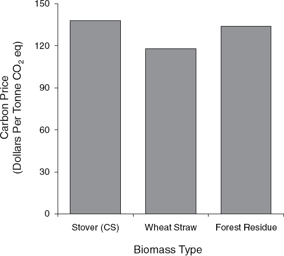
NOTE: No policy incentives ($111 per barrel oil, 70 gallons per dry ton, 23.4 mpgge, 2010 biorefinery).
cellulosic ethanol production if carbon credits for GHG reductions were the only policy incentive. The reported carbon prices should not be interpreted as the carbon price needed to meet RFS2. Additional biomass feedstocks beyond corn stover, wheat straw, and forest residue will likely be needed to meet the RFS2 consumption mandate for cellulosic ethanol. Therefore, the carbon price needed to meet the mandate will depend on the price gap and the reductions in carbon emissions from additional feedstocks.32
Advancements in technology and efficiency will decrease the price gap. If biorefinery efficiency increases to GREET 2020 default assumptions, the ethanol conversion rate increases to 80 gallons per dry ton of feedstock, and the fuel economy increased to 25.4 mpgge for conventional and flex-fuel vehicles, then the carbon price drops by $18 to $24 per
______________
32 With the exception of short-rotation woody crops, dedicated bioenergy feedstocks considered earlier in this chapter have a significantly larger price gap than the three feedstocks considered in the carbon pricing analysis. If carbon emissions reductions from (more expensive) dedicated bioenergy crops are compared to the emissions reductions from corn stover, wheat straw, or forest residue, the carbon price needed to meet the RFS2 mandate will be significantly higher than the crop and woody residue values reported in Figure 4-23. Lower emissions reductions would only exacerbate this effect and result in a significantly higher carbon price while higher emissions reductions would reduce the carbon price needed to meet RFS2.
tonne for a resulting carbon price between $100 and $120 per tonne CO2 eq.33 The estimated carbon price is sensitive to technological progress, such as biorefinery and fuel efficiency, and to the parameter values influencing breakeven values for the biomass processor and supplier, including the oil price, regional biomass productivity, and parameter variability.
Interaction with Agricultural and Forestry Offsets
Under a national carbon policy, biofuels would not be the only way to reduce carbon. Another means that could be encouraged is using agricultural land or forestry to supply carbon credits to carbon markets. These credits have come be to known as “offsets,” given that they are often assumed to be used to offset emissions of carbon dioxide from the energy sector. Offsets work by reducing GHG emissions from some activity in the agricultural or forestry sector or by increasing the carbon stored in soils or forest biomass. Examples of activities that potentially generate offsets include conversion of land to forests (afforestation), extending timber rotations, increasing forest management, shifting from conventional tillage to no tillage, reducing methane (CH4) emissions from livestock operations, reducing fossil fuel use associated with agriculture, and reducing nitrogen oxide emissions from production agriculture (EPA, 2005). The amount of carbon offset by feedstocks differs with the type of crop, previous land uses, crop management, and agrichemical use.
Environmental policies that encourage carbon offsets in agriculture or forestry will have important interactions with biofuel policies because they could influence the total amount of land devoted to forest or agricultural production. A number of studies have examined the implications of offsets for land use in the United States. One of the most important effects relates to the potential for land-use change, and specifically for conversion of land into forests. A model by EPA (2005) suggested that up to 90 million acres of crop and pastureland could be converted to forestland if carbon prices are in the range of $15-$50 per tonne of CO2 eq. Results from Sohngen (2010) suggest similarly large changes in land use, around 100 million acres of new forestland by 2050 with carbon prices of $30 per tonne CO2 eq.34 These studies assume one of two types of carbon payment regimes, either a carbon rental regime that makes rental payments as carbon is stored in forests and a payment for storage in wood products or a subsidy for storage and a tax for the net emission at harvest. Note that these two payment schemes are equivalent in present value terms for newly planted forests. In both these studies, the changes in land use described above are net of all underlying changes. New forests are derived from a combination of crop, pasture, and rangeland. Additional land-use changes outside the United States are captured by the global study by Sohngen (2010) but not by the EPA (2005) study. The scale of the changes in land use associated with carbon policies suggests that the overall value for land would increase dramatically if carbon policies were implemented.
Such large shifts in land use occur with carbon offset policies because offsets in forestry are particularly valuable. Consider a typical acre of cropland in the Eastern Corn Belt. The accumulation of carbon if land is converted to mixed hardwoods could be as much as 4 tonnes CO2 eq per acre per year (Figure 4-24). Further, the carbon in the mixed hardwoods
______________
33 Further, if fuel cell vehicle technology operating on pure ethanol (E100) is available by 2020, the carbon price would decrease to range between $54 to $68 per tonne CO2eq assuming a fuel economy of 44.3 mpgge for fuel cell vehicles and a conversion yield of 80 gallons per dry ton of feedstock.
34 Those model projections must be interpreted in the context of recent changes in land-use patterns in the United States. From 1982 to 2007, cultivated cropland declined by 70 million acres (from 375 million to 305 million acres), developed land increased by 40 million acres (from 71 million to 111 million acres), and there was little change in forestland, pastureland, rangeland, and noncultivated cropland (USDA, 2009).
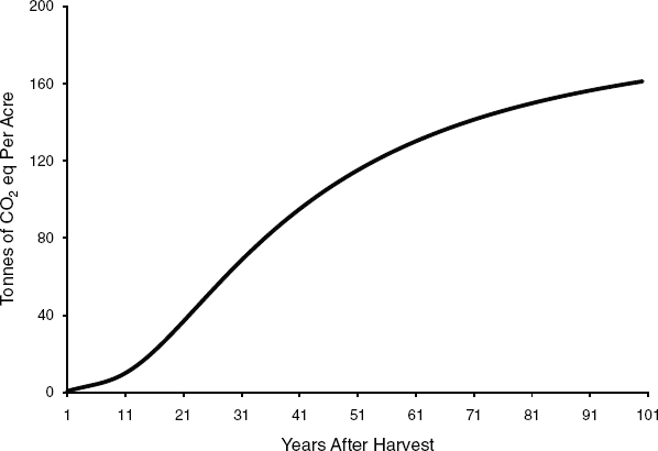
can be observed, as it is stored in trees growing on the landscape. The value of the carbon asset in an acre of trees with a carbon price of $15 per tonne CO2 eq would be $1,350 per acre, assuming a discount rate of 5 percent. Compared to a timber value of about $250 per acre with current timber prices, carbon markets could provide strong incentives for land conversion. Note that these calculations of land value assume that timber is harvested with and without carbon values, although when carbon is valued, the economically optimal rotation age increases from 52 to 63 years of age.
Other types of offsets, such as those that reduce CH4 emissions and nitrogen oxide emissions, are also valuable, but they do not have a strong influence on the competitive balance between cropland, pasture, and forestland. CH4 recovery in livestock operations is done mainly in confined livestock operations where it makes economic sense to recover the CH4. If the value of carbon offsets is to increase, such systems could influence the returns to animal operations so that the total number of animals could increase, thereby increasing the demand for feed. However, with current values for natural gas, CH4 recovery is not profitable enough to have a large effect on projections of animal units.
In addition to afforestation, forest carbon offsets credits may be developed for other activities in forests, including increasing the rotation age in forests or for increasing the intensity of management in order to increase the total carbon stored on site. For example, in the Midwestern hardwood case examined above, a carbon price of $15 per tonne CO2 eq increased the optimal rotation age from 52 years to 63 years. A number of studies have now shown that these actions are relatively low-cost options for storing carbon in forests
Unlike annual agricultural crops, forests produce output periodically. In North America, rotations can be fairly long, ranging from 8-10 years for short-rotation woody crops to 20-30 years for Southern pines to 40-50 years for Douglas Fir in the Pacific Northwest. An interesting question from the perspective of providing a stable supply of biomass relates to determining the optimal timber rotation. Optimal timber rotations are most often determined in terms of maximizing the value of the land and not in terms of maximizing timber supply. Due to discounting, maximizing value implies less output than maximizing output.
Southern pine and poplar, two alternatives for a productive site in the Southern United States, were compared to show the effect of maximizing value. For this example, it was assumed that productivity of the site is the same for both tree types, so they will have approximately the same maximum annual growth. Growth functions of the following functional form were developed for these two tree types:
Southern pine: Volume (dry tons/acre) = exp(5.19 – 25.39/AGE)
Poplar: Volume (dry tons/acre) = exp(4.76 – 16.44/AGE)
These growth functions are shown in Figure 4-25. To compare the two types of trees, several measures of growth are of interest. One measure of growth is the maximum periodic, or annual, growth. This is the maximum amount of biomass accumulated in a single year. Because the two types of trees have different growth characteristics, they accumulate biomass at different rates over time, and the maximum accumulation occurs at different time periods (Table 4-7). As noted above, the two tree types are assumed to be grown on the same site and thus subjected to the same soil and climatic conditions. As a result, the maximum rates of growth are constrained to be roughly the same.
Another measure of growth is the average annual growth, which is measured as the total volume divided by the age. This calculation provides a measure of the average annual material harvested per year if the stand were cut at the given age. The maximum average amount of material that could be harvested per year is 2.6 dry tons per acre per year. Because the growth functions have a different shape, the year at which the average annual harvest is maximized is different for each type. For Southern pine, the average annual growth is maximized at 25 years and for hybrid poplar it is maximized at 16 years.
As a landowner, maximizing annual flow is less important than maximizing the value of the land. The value of the land is maximized when the net present value of the stand is maximized. For this analysis, planting costs were assumed to be $243 per acre, and additional management costs were ignored to simplify the analysis. At rotation age, 90 percent of the growing stock biomass was assumed to be removed. For the Southern pine stand, 60 percent is used for sawtimber and is valued at $19.31 per dry ton ($36.50 per m3). The remainder is used for pulp and is valued at $5.15 per dry ton ($9.73 per m3). For hybrid poplar, all the material can be used for sawtimber, although the value of the sawtimber is assumed to be $14.81 per dry ton ($28 per m3). Land value is maximized in 24-year rotations with Southern pine and 14-year rotations with hybrid poplar. Despite lower value for the harvested material, the hybrid poplar has a larger stand value due to the shorter rotations and the ability to produce more solidwood in that shorter time period.
Interestingly, if all this material were converted to biomass feedstock supply at $4.76 per dry ton ($9 per m3), or roughly the pulpwood price, land value would be $277 per acre, or only about 25 percent of the potential value. Lower planting costs could increase the land value, but it is not clear if these lower planting costs could achieve the same stocking densities and biomass production.ea
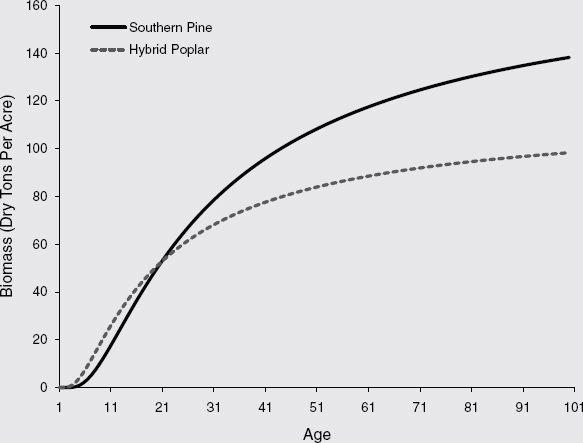
FIGURE 4-25 Growth of growing stock biomass.
TABLE 4-7 Growth Characteristics of Alternative Timber Types
| Southern Pine | Hybrid Poplar | |
| Maximum annual growth in dry tons per acre (age maximized) | 3.82 (13) | 3.84 (9) |
| Average annual growth at year 10 in dry tons per acre | 3.48 | 3.76 |
| Maximum average annual growth in dry tons per acre per year (age maximized) | 2.6 (25) | 2.61 (16) |
| Maximum Net Present Value (NPV) | $854 | $1,123 |
| Rotation age that maximizes NPV | 24 | 14 |
| Average annual flow of biomass at the rotation age that maximizes NPV in dry tons per acre per year | 2.6 | 2.57 |
in the United States, and they could constitute 30 to 50 percent of the total carbon sequestered in the next 30 years (EPA, 2005; Sohngen, 2010). Payments for these activities can be provided to owners with standing timber stocks in order to generate carbon offset credits. Since these incentives value the standing stock of timber, they would serve to increase the value of forests and make standing forests more competitive with other types of land uses, including feedstock production for biofuels. In other words, comprehensive carbon offset policies that pay for offsets through management and increasing timber rotation ages will increase the value of land and make the provision of tons of biomass for bioenergy markets more expensive.
It is difficult at this time to determine what the net effect of both carbon offsets and RFS2 would be on land use. Market studies of carbon offsets imply that additional land converts from livestock and crops to forests under most carbon price scenarios and that the returns to all types of land uses increase, though these studies do not account for the expansion of developed land. The recent EPA study on RFS2 suggests that the area of land used for dedicated bioenergy crops, such as switchgrass, increase, while forestland and rangeland decline. The combination of these results suggests that carbon offsets would compete with cellulosic biofuel production for the same land; thus, environmental policies that encourage carbon offsets could raise the costs of producing cellulosic biofuel feedstocks. Considered a different way, however, this also implies that carbon offsets could limit the negative externalities associated with converting natural forests to dedicated bioenergy crops.
An important caveat to this conclusion occurs if cellulosic biofuel feedstocks are increasingly derived from forest sawtimber and pulpwood supplies rather than residues. In this case, the demand for wood products would increase, timber prices would rise, and land returns in forestry would increase. Because long-term, sustained increases in timber prices raise timber rotation ages over time, and an increase in rotation age expands the supply of timber, in some cases, biofuel outputs and carbon offsets may be complementary.
An additional possible response of markets to increasing biofuel demands is to shift land towards shorter rotation species. Shorter rotations can increase land values, but they do not necessarily increase timber supplies, as discussed in Box 4-6. The key way in which shorter rotations can increase timber supplies occurs if managers are able to manage them better to produce the desired outputs. For instance, there has been a long history of conversion of hardwoods to softwoods in the Southern United States. The key gain here has been an increase in value on the landscape as managers have been better able to control conditions on softwood plantations, and they have been able to obtain higher value output per acre with softwoods than hardwoods. However, net production of biomass on hardwoods is typically greater, but less of it is suitable for high-value market products on a per acre basis (Sohngen and Brown, 2006).
Because cellulosic biofuel is not yet commercially viable, the economics of this type of fuel and its economic effects on other commodities and government programs are speculative. However, with the data that are available and the present state of technology, cellulosic biofuel is not cost-competitive with fossil fuels without government support. Unless more subsidies are used, the RFS2 mandate is enforced rigidly, taxes on petroleum products are increased, or rapid technological advancements are made, cellulosic biofuel will not substantially affect other commodity markets, though it could have repercussions for the federal budget. If cellulosic biofuel becomes commercially viable, land prices will increase due to competition with other agricultural or forestry uses, though the extent of the increase
due to biofuels will depend on the productivity of the land used for biomass production as well as demand for other uses of the land. Fossil fuel prices may decline slightly and imports will decrease, but this will also be influenced by improved fuel efficiency in the U.S. vehicle fleet and the capacity of the U.S. fleet to use biofuels. Because of its scarcity and its density, more woody biomass may be imported to meet the demand for biofuels and traditional uses.
Corn-grain ethanol and, to a lesser extent, soybean biodiesel are closer to being competitive with fossil fuels, particularly when combined with the tax credit and encouraged by RFS2. They have contributed to upward price pressure on agricultural commodities, food, and livestock feed; however, they are just one factor among many, including the growing global population, crop failures in other countries, decline in the value of the U.S. dollar, and speculative activity in the marketplace. The greater use of DDGS in animal feed to some extent has muted the unfavorable effects on the livestock industry.
If policies that were in place at the time this report was written are continued, it is extremely likely that meeting RFS2 will increase the federal budget, particularly in terms of subsidies spent on grants, loans, and loan guarantees to encourage cellulosic biofuel production and in terms of tax revenue forgone by the tax credits for blending biofuel with fossil fuels. To the extent that biofuel policy has raised food-related prices, it has affected federal spending in programs related to agriculture and food. Deciphering biofuels’ contribution to increases or decreases in these programs is difficult, though, because of the number of variables. The effect of RFS2 on federal spending on conservation programs is uncertain. It remains to be seen whether biofuel feedstock production competes with acres or payments for CRP.
Abbott, C. 2010. U.S. Biofuels Hurt if 2010 Tax Break Expires—Report. Available online at http://www.reuters.com/article/2010/03/09/biofuels-usa-taxbreak-idUSN0924548320100309. Accessed February 10, 2011.
Abbott, P.C., C. Hurt, and W.E. Tyner. 2009. What’s Driving Food Prices? March 2009 Update. Oak Brook, IL: Farm Foundation.
Abbott, P.C., C. Hurt, and W.E. Tyner. 2011. What’s Driving Food Prices in 2011? Oak Brook, IL: Farm Foundation.
Aden, A., M. Ruth, K. Ibsen, J. Jechura, K. Neeves, J. Sheehan, B. Wallace, L. Montague, A. Slayton, and J. Lukas. 2002. Lignocellulosic Biomass to Ethanol Process Design and Economics Utilizing Co-Current Dilute Acid Prehydrolysis and Enzymatic Hydrolysis for Corn Stover. Golden, CO: National Renewable Energy Laboratory.
Anex, R.P., A. Aden, F.K. Kazi, J. Fortman, R.M. Swanson, M.M. Wright, J.A. Satrio, R.C. Brown, D.E. Daugaard, A. Platon, G. Kothandaraman, D.D. Hsu, and A. Dutta. 2010. Techno-economic comparison of biomass-to-transportation fuels via pyrolysis, gasification, and biochemical pathways. Fuel 89(Supplement 1):S29-S35.
Babcock, B., S. Marette, and D. Treguer. 2011. Opportunity for profitable investments in cellulosic biofuels. Energy Policy 39:714-719.
Babcock, B.A., and J.F. Fabiosa. 2011. The Impact of Ethanol and Ethanol Subsidies on Corn Prices: Revisiting History. Ames: Iowa State University - Center for Agricultural and Rural Development.
Babcock, B.A., K. Barr, and M. Carriquiry. 2010. Costs and Benefits to Taxpayers, Consumers, and Producers from U.S. Ethanol Policies. Ames: Iowa State University - Center for Agricultural and Rural Development.
Baffes, J., and T. Haniotis. 2010. Placing the 2006/08 Commodity Price Boom into Perspective. Washington, DC: The World Bank.
Baier, S., M. Clements, C. Griffiths, and J. Ihrig. 2009. Biofuels Impact on Crop and Food Prices: Using an Interactive Spreadsheet. Washington, DC: Board of Governors of the Federal Reserve System.
Banse, M., H. van Mejil, A. Tabeau, and G. Woltjer. 2008. Will EU biofuel policies affect global agricultural markets? European Review of Agricultural Economics 35(2):117-141.
Becker, D., P. Jakes, D. Abbas, K.E. Halvorsen, P.J. Jakes, S.M. McCaffrey, and C. Moseley. 2009. Characterizing Lessons Learned from Federal Biomass Removal Projects. Boise, ID: Joint Fire Science Program.
Bengston, D.N., and Z. Xu. 1995. Changing National Forest Values: A Content Analysis. St. Paul, MN: U.S. Department of Agriculture - Forest Service.
Bengston, D.N., T.J. Webb, and D.P. Fan. 2004. Shifting forest value orientations in the United States, 1980–2001: A computer content analysis. Environmental Values 13(3):373-392.
Cai, X., X. Zhang, and D. Wang. 2011. Land availability for biofuel production. Environmental Science & Technology 45(1):334-339.
Capehart, T., and J. Richardson. 2008. Food Price Inflation: Causes and Impacts. Washington, DC: Congressional Research Service.
CBO (Congressional Budget Office). 2009. The Impact of Ethanol Use on Food Prices and Greenhouse-Gas Emissions. Washington, DC: Congressional Budget Office.
CBO (Congressional Budget Office). 2010. Using Biofuel Tax Credits to Achieve Energy and Environmental Policy Goals. Washington, DC: Congressional Budget Office.
Collett, S., and P. Villega, eds. 2005. The Poultry Informed Professional. Issue 85:July/August. Athens: The University of Georgia.
Collett, S., and P. Villega, eds. 2008. The Poultry Informed Professional. Issue 99:May/June. Athens: The University of Georgia.
Collett, S., and P. Villega, eds. 2011. The Poultry Informed Professional. Issue 118:May/June. Athens: The University of Georgia.
Collins, K. 2008. The Role of Biofuels and Other Factors in Increasing Farm and Food Prices: A Review of Recent Developments with a Focus on Feed Grain Markets and Market Prospects. Northfield, IL: Kraft Food Global, Inc.
Cotti, C., and M. Skidmore. 2010. The impact of state government subsidies and tax credits in an emerging industry: Ethanol production 1980-2007. Southern Economic Journal 76(4):1076-1093.
Cowan, T. 2010. Conservation Reserve Program: Status and Current Issues. Washington, DC: Congressional Research Service.
Crompton, J. 2008. Food Bank Crisis: Funding Cutbacks Cripple Efforts to Feed the Hungry. Available online at http://www.post-gazette.com/pg/08104/872253-58.stm. Accessed November 2, 2010.
Cubbage, F., S. Koesbandana, P. Mac Donagh, R. Rubilar, G. Balmelli, V.M. Olmos, R. De La Torre, M. Murara, V.A. Hoeflich, H. Kotze, R. Gonzalez, O. Carrero, G. Frey, T. Adams, J. Turner, R. Lord, J. Huang, C. MacIntyre, K. McGinley, R. Abt, and R. Phillips. 2010. Global timber investments, wood costs, regulation, and risk. Biomass and Bioenergy 34(12):1667-1678.
de Gorter, H., and D.R. Just. 2010. The social costs and benefits of biofuels: The intersection of environmental, energy and agricultural policy. Applied Economic Perspectives and Policy 32(1):4-32.
de Groot, R.S., M.A. Wilson, and R.M.J. Boumans. 2002. A typology for the classification, description and valuation of ecosystem functions, goods and services. Ecological Economics 41(3):393-408.
Dietz, T., A. Dan, and R. Shwom. 2007. Support for climate change policy: Social psychological and social structural influences. Rural Sociology 72(2):185-214.
Donohue, M., and D.L. Cunningham. 2009. Effects of grain and oilseed prices on the costs of U.S. poultry production. Journal of Applied Poultry Research 18(2):325-337.
Duffield, J.A., I. Xiarchos, and S.A. Halbrook. 2008. Ethanol policy: Past, present, and future. South Dakota Law Review 53(3):425-456.
Dunlap, R.E. 2010. Climate change and rural sociology: Broadening the research agenda. Rural Sociology 75(1):17-27.
Dunlap, R.E., and K.D. Van Liere. 1978. The “new environmental paradigm”: A proposed measuring instrument and preliminary results. Journal of Environmental Education 9(4):10-19.
EIA (U.S. Energy Information Administration). 2008a. Annual Energy Outlook 2008. Washington, DC: U.S. Department of Energy - Energy Information Administration.
EIA (U.S. Energy Information Administration). 2008b. Federal Financial Interventions and Subsidies in Energy Markets 2007. Washington, DC: U.S. Department of Energy - Energy Information Administration.
EIA (U.S. Energy Information Administration). 2010a. Annual Energy Outlook 2010—With Projections to 2035. Washington, DC: U.S. Department of Energy - Energy Information Administration.
EIA (U.S. Energy Information Administration). 2010b. Annual Energy Review 2009. Washington, DC: U.S. Department of Energy - Energy Information Administration.
EIA (U.S. Energy Information Administration). 2010c. Petroleum and other liquids: Cushing, OK WTI spot price FOB (Dollars per Barrel). Available online at http://www.eia.doe.gov/dnav/pet/hist/LeafHandler.ashx?n=PET&s=RWTC&f=D. Accessed September 20, 2011.
EPA (U.S. Environmental Protection Agency). 2005. Greenhouse Gas Mitigation Potential in U.S. Forestry and Agriculture. Washington, DC: U.S. Environmental Protection Agency.
EPA (U.S. Environmental Protection Agency). 2010. Renewable Fuel Standard Program (RFS2) Regulatory Impact Analysis. Washington, DC: U.S. Environmental Protection Agency.
Espey, M. 1996. Explaining the variation in elasticity estimates of gasoline demand in the United States: A meta-analysis. Energy Journal 17(3):49-60.
Espey, M. 1998. Gasoline demand revisited: An international meta-analysis of elasticities. Energy Economics 20(3):273-295.
FAPRI (Food and Agricultural Policy Research Institute). 2010. U.S. Baseline Briefing Book: Projections for Agricultural and Biofuel Markets. Columbia: University of Missouri-Columbia.
Fight, R.D., B.R. Hartsough, and P. Noordijk. 2006. Users Guide for FRCS: Fuel Reduction Cost Simulator Software. Portland, OR: U.S. Department of Agriculture - Forest Service.
Fischer, G., E. Hizsnyik, S. Prieler, M. Shah, and H. van Velthuizen. 2009. Biofuels and Food Security. Vienna, Austria: OPEC Fund for International Development / International Institute for Applied Systems Analysis.
Forest2Market. 2010. Delivered Price Benchmark Service. Available online at http://www.forest2market.com/. Accessed February 14, 2011.
French, B.C. 1960. Some considerations in estimating assembly cost functions for agricultural processing operations. Journal of Farm Economics 42(4):767-778.
Galik, C.S., R. Abt, and Y. Wu. 2009. Forest biomass supply in the southeastern United States—Implications for industrial roundwood and bioenergy production. Journal of Forestry 107(2):69-77.
GAO (U.S. General Accounting Office). 1993. A Glossary of Terms Used in the Federal Budget Process. Washington: U.S. General Accounting Office.
GAO (U.S. General Accounting Office). 2004. Principles of Federal Appropriations Law. Washington: U.S. General Accounting Office.
GAO (U.S. Government Accountability Office). 2011. Opportunities to Reduce Potential Duplication in Government Programs, Save Tax Dollars, and Enhance Revenue. Washington: U.S. Government Accountability Office.
Gardner, B.L. 1975. Farm retail price spread in a competitive food-industry. American Journal of Agricultural Economics 57(3):399-409.
Gardner, B.L. 1987. The Economics of Agricultural Policies. New York: Macmillan.
Gehlhar, M., A. Winston, and A. Somwaru. 2010. Effects of Increased Biofuels on the U.S. Economy in 2022. Washington, DC: U.S. Department of Agriculture - Economic Research Service.
Glauber, J. 2008. Full Committee Hearing to Receive Testimony on the Relationship between U.S. Renewable Fuels Policy and Food Prices before the Senate Committee on Energy and Natural Resources, June 12.
Goodwin, P., J. Dargay, and M. Hanly. 2004. Elasticities of road traffic and fuel consumption with respect to price and income: A review. Transport Reviews 24(3):275-292.
Graham, D.J., and S. Glaister. 2002. The demand for automobile fuel: A survey of elasticities. Journal of Transport Economics and Policy 36(1):1-25.
Haynes, R.W. 2003. An Analysis of the Timber Situation in the United States: 1952 to 2050. Portland, OR: U.S. Department of Agriculture - Forest Service.
Haynes, R.W. 2008. Emergent Lessons from a Century of Experience with Pacific Northwest Timber Markets. Portland, OR: U.S. Department of Agriculture, Forest Service.
Heaton, E.A., S.P. Long, T.B. Voigt, M.B. Jones, and J. Clifton-Brown. 2004. Miscanthus for renewable energy generation: European Union experience and projections for Illinois. Mitigation and Adaptation Strategies for Global Change 9(4):433-451.
Hertel, T.W., and J.F. Beckman. 2010. Commodity price volatility in the biofuel era: An examination of the linkage between energy and agricultural markets. Paper read at the 2010 Annual Agricultural and Applied Economics Association Meeting, July 25-27, Denver, CO.
Hertel, T.W., W.E. Tyner, and D.K. Birur. 2010. The global impacts of biofuel mandates. Energy Journal 31(1):75-100.
Howard, J.L. 2007. U.S. Timber Production, Trade, Consumption, and Price Statistics 1965 to 2005. Madison, WI: U.S. Department of Agriculture - Forest Service.
Huang, H.-J., S. Ramaswamy, W. Al-Dajani, U. Tschirner, and R.A. Cairncross. 2009. Effect of biomass species and plant size on cellulosic ethanol: A comparative process and economic analysis. Biomass and Bioenergy 33(2):234-246.
IMF (International Monetary Fund). 2008. Is inflation back? Commodity prices and inflation in World Economic Outlook, October 2008: Financial Stress, Downturns, and Recoveries. Washington, DC: International Monetary Fund.
IMF (International Monetary Fund). 2010. IMF primary commodity prices. Available online at http://www.imf.org/external/np/res/commod/index.asp. Accessed September 22, 2010.
ISUE (Iowa State University Extension). 2010. Decision Tools—Crop Decisions. Available online at http://www.extension.iastate.edu/agdm/decisionaidscd.html. Accessed February, 1, 2011.
Jenkins, B.M., R.B. Williams, N. Parker, P. Tittmann, Q. Hart, M.C. Gildart, S. Kaffka, B.R. Hartsough, and P. Dempster. 2009. Sustainable use of California biomass resources can help meet state and national bioenergy targets. California Agriculture 63(4):168-177.
Jensen, H.H., and B.A. Babcock. 2007. Do biofuels mean inexpensive food is a thing of the past? Iowa Ag Review 13(3):4-5, 11.
Jiang, Y., and S.M. Swinton. 2009. Market interactions, farmer choices, and the sustainability of growing advanced biofuels: A missing perspective? International Journal of Sustainable Development and World Ecology 16(6):438-450.
Johnson, D.M., K.E. Halvorsen, and B.D. Solomen. 2011. Upper midwestern U.S. consumers and ethanol: Knowledge, beliefs and consumption. Biomass and Bioenergy 35(4):1454-1464.
Johnson, S. 2008. Commodity Prices: Outlook and Risks. Washington, DC: International Monetary Fund.
Kempton, W., J.S. Boster, and J.A. Hartley. 1996. Environmental Values in American Culture. 1st MIT Press, pbk. ed. Cambridge, MA: MIT Press.
Khanna, M. 2008. Cellulosic biofuels: Are they economically viable and environmentally sustainable? Choices 23(3):16-23.
Khanna, M., and B. Dhungana. 2007. Economics of alternative feedstocks. Pp. 129–146 in Corn-Based Ethanol in Illinois and the U.S.: A Report from the Department of Agricultural and Consumer Economics, University of Illinois. Urbana-Champaign: University of Illinois.
Khanna, M., B. Dhungana, and J. Clifton-Brown. 2008. Costs of producing Miscanthus and switchgrass for bioenergy in Illinois. Biomass and Bioenergy 32(6):482-493.
Khanna, M., X. Chen, H. Huang, and H. Onal. 2010. Supply of cellulosic biofuel feedstocks and regional production patterns. American Journal of Agricultural Economics 93(2):472-280.
Kior. 2011. SEC Filings. Available online at http://investor.kior.com/sec.cfm. Accessed August 1, 2011.
Kløverpris, J., H. Wenzel, and P. Nielsen. 2008. Life cycle inventory modelling of land use induced by crop consumption. The International Journal of Life Cycle Assessment 13(1):13-21.
Koplow, D. 2009. State and federal subsidies to biofuels: Magnitude and options for redirection. International Journal of Biotechnology 11(1/2):92-126.
Lazear, E. 2008. Hearing on Responding to the Global Food Crisis before the Senate Foreign Relations Committee, May 14.
Leibtag, E. 2008. Corn prices near record high, but what about food costs? Amber Waves 6(February):11-15.
Lipsky, J. 2008. Commodity Prices and Global Inflation: Remarks to the Council on Foreign Relations, May 8, New York City.
Lustig, N. 2008. Thought for Food: The Challenges of Coping with Soaring Food Prices. Washington, DC: Center for Global Development.
Manomet (Manomet Center for Conservation Sciences). 2010. Massachusetts Biomass Sustainability and Carbon Policy Study: Report to the Commonwealth of Massachusetts Department of Energy Resources. Brunswick, ME: Manomet Center for Conservation Sciences.
Miranowski, J., and A. Rosburg. 2010. Using cellulosic ethanol to “go green”: What price for carbon? Paper read at the 2010 Annual Agricultural and Applied Economics Association, July 25–27, Denver, CO.
Miranowski, J., M. Khanna, and J.R. Hess. 2011. Economic of feedstock production, harvest, storage, and transport. Proceedings of the Sustainable Feedstocks for Advanced Biofuels Workshop.
Mitchell, D. 2008. A Note on Rising Food Prices. Washington, DC: The World Bank.
NAS-NAE-NRC (National Academy of Sciences, National Academy of Engineering, National Research Council). 2009a. America’s Energy Future: Technology and Transformation. Washington, DC: National Academies Press.
NAS-NAE-NRC (National Academy of Sciences, National Academy of Engineering, National Research Council). 2009b. Liquid Transportation Fuels from Coal and Biomass: Technological Status, Costs, and Environmental Impacts. Washington, DC: National Academies Press.
Neeley, T. 2010. Biodiesel industry asks for reinstatement of tax credit before election. Available online at http://www.dtnprogressivefarmer.com/dtnag/view/blog/getBlog.do;jsessionid=6798D52B11E8AD50A8797C9AD6AB4F3A.agfreejvm2?blogHandle=ethanol&blogEntryId=8a82c0bc2a8c8730012b445bc23e08ec. Accessed February 10, 2011.
NHDRA (New Hampshire Department of Revenue Administration). 2010. Average Stumpage Value List. Concord: New Hampshire Department of Revenue Administration.
OMB (Office of Management and Budget). 2010. Budget of the U.S. Government: Fiscal Year 2011—The Budget. Available online at http://www.whitehouse.gov/omb/budget/Overview. Accessed October 26, 2010.
Perlack, R.D., and B.J. Stokes (Leads). 2011. U.S. Billion-Ton Update: Biomass Supply for a Bioenergy and Bioproducts Industry. Oak Ridge, TN: Oak Ridge National Laboratory.
Perlack, R.D., L.L. Wright, A.F. Turhollow, R.L. Graham, B.J. Stokes, and D.C. Erbach. 2005. Biomass as Feedstock for a Bioenergy and Bioproducts Industry: The Technical Feasibility of a Billion-Ton Annual Supply. Washington, DC: U.S. Department of Energy and U.S. Department of Agriculture.
Perrin, R.K. 2008. Ethanol and food prices: Preliminary assessment. Lincoln: University of Nebraska.
Reinbold, D. 2008. Price Increases Keep Local Food Banks Busy. Available online at http://voicesweb.org/node/1674. Accessed November 2, 2010.
Roland-Holst, D. 2010. Will emerging markets decide the food-fuel debate? Presentation to the Committee on Economic and Environmental Effects of Increasing Biofuels Production on October 7.
Rosegrant, M.W. 2008. Hearing on Biofuels and Grain Prices: Impacts and Policy Responses before the Senate Committee on Homeland Security and Governmental Affairs, May 7.
Ruttan, V.W. 1982. Agricultural Research Policy. Minneapolis: University of Minnesota Press.
Schick, A. 2000. The Federal Budget: Politics, Policy, Process. Revised ed. Washington, DC: Brookings Institution Press.
Schmit, T.M., R.N. Boisvert, D. Enahoro, and L.E. Chase. 2009. Optimal dairy farm adjustments to increased utilization of corn distillers dried grains with solubles. Journal of Dairy Science 92(12):6105-6115.
Sedjo, R.A. 2010. The Biomass Crop Assistance Program (BCAP): Some Implications for the Forest Industry. Washington, DC: Resources for the Future.
Sedjo, R.A., and B. Sohngen. 2009. The Implications of Increased Use of Wood for Biofuel Production. Washington, DC: Resources for the Future.
Smith, C.E. 2010. Special Report; Pipeline construction plans slow for 2010. Available online at http://www.ogj.com/articles/print/volume-108/issue-6/technology/special-report-pipeline.html. Accessed March 8, 2010.
Sohngen, B. 2010. Forestry carbon sequestration. Pp. 114-141 in Smart Solutions to Climate Change: Comparing Costs and Benefits, B. Lomborg, ed. Cambridge: Cambridge University Press.
Sohngen, B., and S. Brown. 2006. The influence of conversion of forest types on carbon sequestration and other ecosystem services in the south central United States. Ecological Economics 57(4):698-708.
Sohngen, B.L., and R.W. Haynes. 1994. The “Great” Price Spike Of ’93: An Analysis of Lumber and Stumpage Prices in the Pacific Northwest. Portland, OR: U.S. Department of Agriculture - Forest Service.
Sohngen, B., J. Anderson, S. Petrova, and K. Goslee. 2010. Alder Springs Biomass Removal Economic Analysis. Arlington, VA: Winrock International and U.S. Department of Agriculture - Forest Service.
Solomon, B.D., and N.H. Johnson. 2009. Valuing climate protection through willingness to pay for biomass ethanol. Ecological Economics 68(7):2137-2144.
Solomon, B.D., J.R. Barnes, and K.E. Halvorsen. 2007. Grain and cellulosic ethanol: History, economics, and energy policy. Biomass and Bioenergy 31(6):416-425.
Spelter, H., and D. Toth. 2009. North America’s Wood Pellet Sector. Madison, WI: U.S. Department of Agriculture - Forest Service.
Stebbins, C. 2011. Analysis: U.S. biodiesel on life support, but smiling. Available online at http://www.reuters.com/article/2011/02/04/us-usa-bi0diesel-idUSTRE7130H920110204?feedType=RSS&feedName=GCA-GreenBusiness. Accessed February 10, 2011.
Steenblik, R. 2007. Biofuels—At What Cost? Government Support for Ethanol and Biodiesel in Selected OECD Countries. Winnipeg, Canada: International Institute for Sustainable Development.
Stubbs, M. 2010. Biomass Crop Assistance Program (BCAP): Status and Issues. Washington, DC: Congressional Research Service.
Swanson, R.M., J.A. Satrio, R.C. Brown, and D.D. Hsu. 2010. Techno-Economic Analysis of Biofuels Production Based on Gasification. Golden, CO: National Renewable Energy Laboratory.
Swinton, S.M., B.A. Babcock, L.K. James, and V. Bandaru. 2011. Higher US crop prices trigger little area expansion so marginal land for biofuel crops is limited. Energy Policy 39:5254-5258.
Taheripour, F., T.W. Hertel, and W.E. Tyner. 2010. Implications of biofuels mandates for the global livestock industry: A computable general equilibrium analysis. Agricultural Economics 10.1111/j.1574-0862.2010.00517.x:1-18.
TCPA (Texas Comptroller of Public Accounts). 2008. Government financial subsidies. Pp. 367-402 in The Energy Report 2008. Austin: Texas Comptroller of Public Accounts.
Timber-Mart South. 2010. South-wide Average Prices Available online at http://www.tmart-south.com/prices.html. Accessed February 14, 2011.
Timilsina, G.R., and A. Shrestha. 2010. Biofuels: Markets, Targets and Impacts. Washington, DC: The World Bank.
Tomek, W.G., and K.L. Robinson. 1983. Agricultural Product Prices. Ithaca, NY: Cornell University Press.
Trostle, R. 2008. Global Agricultural Supply and Demand: Factors Contributing to the Recent Increase in Food Commodity Prices. Washington, DC: U.S. Department of Agriculture - Economic Research Service.
Tyner, W.E. 2008. The U.S. ethanol and biofuels boom: Its origins, current status, and future prospects. BioScience 58(7):646-653.
U.S. Census Bureau. 2010. New Residential Construction: Building Permits, Housing Starts, and Housing Completions. Available online at http://www.census.gov/const/www/newresconstindex.html#. Accessed November 9, 2010.
USDA (U.S. Department of Agriculture). 2009. Summary Report: 2007 National Resources Inventory. Washington, DC, and Ames, Iowa: U.S. Department of Agriculture - Natural Resources Conservation Service and Center for Survey Statistics and Methodology.
USDA (U.S. Department of Agriculture). 2011. USDA Agricultural Projections to 2020. Washington, DC: U.S. Department of Agriculture.
USDA-ERS (U.S. Department of Agriculture - Economic Research Service). 2007. Major Land Uses: U.S. Cropland Used for Crops. Available online at http://www.ers.usda.gov/Data/MajorLandUses/. Accessed February 14, 2011.
USDA-ERS (U.S. Department of Agriculture - Economic Research Service). 2011a. Feed Grains Database: Custom Queries. Available online at http://www.ers.usda.gov/Data/Feedgrains/CustomQuery/. Accessed August 29, 2011.
USDA-ERS (U.S. Department of Agriculture - Economic Research Service). 2011b. Food CPI and Expenditures: Analysis and Forecasts of the CPI for Food. Available online at http://www.ers.usda.gov/Briefing/CPIFoodAndExpenditures/consumerpriceindex.htm. Accessed February 10, 2011.
USDA-ERS (U.S. Department of Agriculture - Economic Research Service). 2011c. Price Spreads from Farm to Consumer: Marketing Bill and Farm Value Components of Consumer Expenditures for Domestically Produced Farm Foods. Available online at http://www.ers.usda.gov/Data/FarmToConsumer/Data/marketingbilltable1.htm. Accessed February 20, 2011.
USDA-FAS (U.S. Department of Agriculture - Foreign Agricultural Service). 2010. Data: Current and Archived Reports. Available online at http://www.fas.usda.gov/data.asp. Accessed February 8, 2011.
USDA-NASS (U.S. Department of Agriculture - National Agricultural Statistics Service). 2007a. Agricultural Prices. Washington, DC: U.S. Department of Agriculture - National Agricultural Statistics Service.
USDA-NASS (U.S. Department of Agriculture - National Agricultural Statistics Service). 2007b. Agricultural Prices: 2006 Summary. Washington, DC: U.S. Department of Agriculture - National Agricultural Statistics Service.
USDA-NASS (U.S. Department of Agriculture - National Agricultural Statistics Service). 2010. Data and Statistics: Quick Stats. Available online at http://www.nass.usda.gov/Data_and_Statistics/Quick_Stats/index.asp. Accessed February 14, 2011.
USITC (U.S. International Trade Commission). 2009. The Economic Effects of Significant U.S. Import Restraints. Sixth Update, 2009. Washington, DC: U.S. International Trade Commission.
USITC (U.S. International Trade Commission). 2010a. Harmonized Tariff Schedule of the United States (2010) (Rev. 2). Washington, DC: U.S. International Trade Commission.
USITC (U.S. International Trade Commission). 2010b. USITC Interactive Tariff and Trade DataWeb. Available online at http://www.dataweb.usitc.gov/. Accessed February 14, 2011.
von Braun, J. 2008. High and rising food prices: Why are they rising, who is affected, how are they affected, and what should be done? Paper read at the U.S. Agency for International Development Conference on Addressing the Challenges of a Changing World Food Situation: Preventing Crisis and Leveraging Opportunity, April 11, Washington, DC.
Warren, D.D. 2010. Production, Prices, Employment, and Trade in Northwest Forest Industries, All Quarters 2009. Portland, OR: U.S. Department of Agriculture - Forest Service.
Wiggins, S., and S. Levy. 2008. Rising Food Prices: A Global Crisis. London: Overseas Development Institute.
Wilson, M.A., and S.R. Carpenter. 1999. Economic valuation of freshwater ecosystem services in the United States: 1971-1997. Ecological Applications 9(3):772-783.
Wise, M., K. Calvin, A. Thomson, L. Clarke, B. Bond-Lamberty, R. Sands, S.J. Smith, A. Janetos, and J. Edmonds. 2009. Implications of limiting CO2 concentrations for land use and energy. Science 324(5931):1183-1186.
Wright, M.M., and R.C. Brown. 2007. Comparative economics of biorefineries based on the biochemical and thermochemical platforms. Biofuels, Bioproducts and Biorefining 1(1):49-56.
Wright, M.M., J.A. Satrio, R.C. Brown, D.E. Saugaard, and D.D. Hsu. 2010. Techno-Economic Analysis of Biomass Fast Pyrolysis to Transportation Fuels. Golden, CO: National Renewable Energy Laboratory.
Xu, Z., and D.N. Bengston. 1997. Trends in national forest values among forestry professionals, environmentalists, and the news media, 1982-1993. Society and Natural Resources: An International Journal 10(1):43-59.


