
3
Climate Transitions, Tipping Points, and the Point of No Return
Because of the extended timescale—several centuries—necessary for climate to adjust to an increase in atmospheric CO2, the current icehouse climate is out of equilibrium with long-term CO2 forcing (Hansen et al., 2008). As the planet continues to warm, it may be approaching a critical climate threshold beyond which rapid (decadal-scale) and potentially catastrophic changes may occur that are not anticipated—because of complex feedback dynamics and existing computational limitations—by climate models that are tuned to modern conditions. This chapter focuses on the insights that can be gleaned from the deep-time geological archive of climate change concerning such thresholds, with particular focus on the major societal questions noted in Chapter 1: How soon, abrupt, and dramatic will climate change be, and how long will the new climate states persist?
Climate modeling efforts and the geological record provide plenty of evidence for climate system thresholds, or “tipping points” (Box 3.1), beyond which rapid changes can occur without any additional forcing (Hansen et al., 2008; Lenton et al., 2008). Components of the climate system that are particularly vulnerable to being forced by increasing atmospheric CO2 across a threshold into a new state include the loss of Arctic summer sea ice, the stability of the Greenland and West Antarctic ice sheets, the vigor of the meridional overturning circulation in the North Atlantic and around Antarctica, the extent of Amazon and boreal forests, and the variability of the El Niño-Southern Oscillation (ENSO) (Lenton et al., 2008). The changes in state across such “tipping points” are typically accelerated relative to the apparent rate of forcing, are accompanied by large-scale
BOX 3.1 Tipping Points and the Point of No Return
There are sound theoretical reasons to think that tipping points across climatic thresholds exist (Gladwell, 2000; NRC, 2002). Examples of threshold behaviors include thermohaline circulation modifications, ice sheet instabilities, sea ice instabilities, soil-moisture feedbacks, and the onset of high-latitude convection and associated high-level cloud forcing. Hansen et al. (2008) introduced the term “tipping element” to describe subcontinental-scale subsystems of the Earth system that are susceptible to being forced into a new state by small perturbations. Tipping level—the magnitude of climate forcing beyond which, if sustained, abrupt climate change will eventually occur—is differentiated from “point of no return.” If the tipping level is exceeded for only a brief period of time, the original state of the system can be restored. More persistent forcing can push the system to the “point of no return,” where a reduction of the forcing below the tipping level is ineffective in halting the climate shift (Figure 3.1). This irreversibility of the system response is referred to as hysteresis (NRC, 2002).
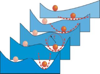
FIGURE 3.1 Equilibrium states of a “system” (valleys) in response to gradual anthropogenic CO2 forcing (progressing from dark to light blue). The curvature of the valley is inversely proportional to the system’s response time (τ) to small perturbations. A threshold is reached when the valley becomes shallower and finally vanishes causing the ball to abruptly roll to a new state (to the left).
SOURCE: Lenton et al. (2008), ©National Academy of Sciences, U.S.A.
impacts on ecological systems, and typically involve hysteresis (Lenton et al., 2008).
ICEHOUSE-GREENHOUSE TRANSITIONS
The following sections describe four periods of past climate change—icehouse-to-greenhouse or greenhouse-to-icehouse transitions—that were driven by slow (long-term) climate forcing across a critical threshold that led to abrupt and highly variable climate responses, as examples of what can be gleaned from the deep-time geological record of climate change and the scientific challenges that persist.
Initiation of the Cenozoic Icehouse
The early Cenozoic greenhouse Earth was plunged from a protracted state of warmth into its current glacial state 33.7 million years ago (Ma), at the Eocene-Oligocene boundary. The transition from a relatively deglaciated climate state to one in which the Antarctic ice sheet grew to between 40 and 160 percent of its modern size occurred within ~200,000 to 300,000 years (Coxall et al., 2005; Liu et al., 2009b). A long-term decrease in CO2, commencing after the Early Eocene Climate Optimum at 52 Ma, has been proposed as the main cause of this cooling trend (Box 3.2) (Edmond and Huh, 2003; Kent and Muttoni, 2008). A CO2 decrease through yet another apparent threshold (from as high as 415 ppmv [parts per million by volume] in the early Pliocene to ~280 ppmv; Pagani et al., 2010; Seki et al., 2010) most probably accounted for the initiation and growth of northern hemisphere ice sheets at around 3 Ma (DeConto et al., 2008; Lunt et al., 2008).
All of the elements of a tipping point climate transition are recorded by this greenhouse-to-icehouse turnover (Kump, 2009). As the climate system reorganized itself, it experienced an overshoot (the Oi-1 climate event) into a deep glacial, which was colder and with larger ice sheets than would be sustained during the less extreme conditions of the glaciated Oligocene (Zachos et al., 1996). The calcium carbonate compensation depth in the oceans deepened substantially in two 40-thousand-year (ky) long steps (separated by 200 ky) that occurred synchronously with the stepwise onset of major permanent ice sheets in Antarctica (Coxall et al., 2005). This instability in the climate system persisted for ~200 to 300 ky (Zachos et al., 2001b) and caused major changes in ocean and atmosphericic circulation with widespread effects on most marine and terrestrial ecosystems (Pearson et al., 2008). Such a characteristic response of a homeostatic feedback system implies an underlying dynamic that still remains to be fully understood but could result from changes in, and the interplay between,
BOX 3.2 Separating the Influence of Ice Volume and Temperature
The gradual cooling from the hothouse of the Early Eocene Climate Optimum (52 Ma) to the onset of Oligocene glaciation in Antarctica (~34 Ma) was first inferred from a long-term global trend of increasing benthic foraminiferal δ18O values (Figure 3.2). The temperature of the deepest water in the oceans—an indication of global climate—was at least 10°C higher in the early Eocene than it is today. The cooling trend was disrupted several times by transient warming events in the Eocene and also by an abrupt shift toward heavier isotopic values (~1 to 1.5‰ [parts per thousand] increase in δ18O in all records) at the Eocene-Oligocene boundary (referred to as the “Oi-1 overshoot”; Zachos et al., 2001b), with this transient cooling a result of some combination of rapid East Antarctic ice sheet growth and global cooling (Zachos et al., 2001a; Coxall et al., 2005). Marine carbon isotope compositions and CaCO3 accumulation rates also exhibit the distinctive “overshoot,” suggesting teleconnections between the southern hemisphere high latitudes and the tropical ocean (Coxall et al., 2005).
A number of additional proxies have been used to separate, or deconvolve, the effects of ice sheet growth from cooling—sequence stratigraphy to assess sea level change (e.g., Kominz and Pekar, 2001); marine geochemical proxies of temperature, including Mg/Ca ratios of foraminiferal calcite (e.g., Lear et al., 2000; Katz et al., 2008) and biomarkers (spores and pollen) in marine sediments (e.g., Liu et al., 2010); as well as terrestrial climate reconstructions based on oxygen isotopes in teeth and bones (e.g., Zanazzi and Kohn, 2008). The latest assessments indicate that the greenhouse-to-icehouse transition occurred in a series of steps with increasing influence of ice volume (Lear et al., 2008) and that cooling preceded ice sheet expansion, with maximum ice sheet size perhaps as much as 15 percent greater than today’s Antarctic ice sheet (Pälike et al., 2006a; Liu et al., 2009b). A threshold was likely reached through a combination of orbitally driven changes in summer insolation and declining atmospheric CO2 levels (DeConto and Pollard, 2003), although oceanic gateway opening and the thermal isolation of Antarctica may have played a role (Barker et al., 2007; Jovane et al., 2007).
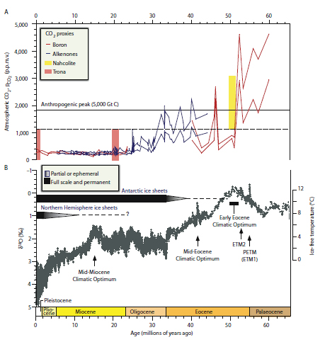
FIGURE 3.2 Relationship between atmospheric CO2 (A) and climate (B) through the Cenozoic. The upper panel shows reconstructed pCO2 from marine and lacustrine proxy records; the dashed line is maximum pCO2 for the Neogene estimated by equilibrium calculations using lacustrine mineral phases (Lowenstein and Demicco, 2006). The climate curve in the lower panel is a composite of deep-sea benthic foraminiferal oxygen-isotope records, smoothed using a five-point running mean (Zachos et al., 2001a, 2008). The temperature scale on the right axis was calculated for an “ice-free ocean,” and is thus applicable solely to the pre-Oligocene portion of record.
SOURCE: Zachos et al. (2008), reprinted by permission of Macmillan Publishers Ltd.
global silicate weathering rates, the global burial rates of marine CaCO3 and siliceous plankton, atmospheric CO2 levels, and ice sheet growth and ablation paced by changes in Earth’s orbit (Coxall et al., 2005; Zachos and Kump, 2005; Pälike et al., 2006a).
The CO2 threshold behavior exhibited by the Eocene-Oligocene onset of Antarctic glaciation and the Neogene initiation of the Greenland ice sheet suggests that multiple equilibrium states exist in the climate system. To the extent that the ice sheet climate system exhibits hysteresis, the CO2 threshold identified for the cooling path may be substantially lower than that for the reverse warming path. Simulations of the modern climate system (DeConto and Pollard, 2003) and empirical proxy records (Pearson et al., 2009) have suggested a substantial delay (up to several millennia) in ice sheet response to increased atmospheric CO2 due to hysteresis. Such studies indicate that polar ice sheet decay may require CO2 levels well above those that existed during the initiation of Cenozoic glaciation (Pollard and DeConto, 2005). Recent evidence, however, indicates the potential for subdecadal response times of ice sheets and much more rapid melting (Das et al., 2008; van de Wal et al., 2008). The response of the Neogene polar ice sheets to the atmospheric CO2 levels during the Middle Miocene climatic optimum (~500 ppmv at 16 Ma; Küerschner et al., 2008) and the early Pliocene (up to 415 ppmv at 4.5 Ma; Pagani et al., 2010)—values not too different from modern (2010) concentrations—warrants further exploration to resolve the uncertainties in ice sheet response times to global warming. If CO2 forcing is sustained at levels through the point of no return, then rapid meltdown of glaciers can be anticipated in the future even if carbon emissions to the atmosphere ultimately decrease (Hansen et al., 2008).
If hysteresis is characteristic of ice sheet melting dynamics, then such a delay in ice sheet response to elevated CO2 guarantees a future transition into a warm world that is abrupt, extreme, and with possibly irreversible catastrophic effects (Hansen et al., 2008; Kump, 2009). Presumably, the long-term processes that drove the climate system into the glacial state during the Cenozoic (enhanced silicate weathering and mountain building, reduced subduction of carbonates and volcanism, and thus low atmospheric CO2 levels) will persist through the anthropogenic perturbation, so it is reasonable to anticipate that the climate—following the current transient warming—will cool over the subsequent few tens of millennia. Eventually, conditions for the reinitiation of the Antarctic and Greenland ice sheets will be achieved, but these may require atmospheric pCO2 levels similar to preindustrial values and a favorable orbital state (Berger et al., 2003; Pollard and DeConto, 2005). Thus, the trip “forward to the past” may be quite prolonged, perhaps approaching the evolutionary timescales of species, including Homo sapiens.
Paleocene-Eocene Thermal Maximum (PETM)
One of the best-known examples of an ancient global warming event, with potential parallels to the near future, is the Paleocene-Eocene Thermal Maximum (PETM). This abrupt climate change occurred at ~56 Ma with repeated, rapid (millennial-scale), massive releases of “fossil” carbon and major disruption of the carbon cycle (Kennett and Stott, 1991, 1995; Dickens et al., 1995; Zachos et al., 2003). The oxygen isotopic compositions of planktonic and benthic foraminifera record rapid warming of ~5°C in tropical surface and deep oceans, and as much as 9°C warming at the poles, that persisted for ~170 ky (Sluijs et al., 2006; Zachos et al., 2006; Röhl et al., 2007) (Figure 3.3). Greenhouse gas-forced global warming was accompanied by extreme changes in hydroclimate and accelerated weathering (Bowen et al., 2004; Pagani et al., 2006; Schmitz and Pujalte, 2007), deep-ocean acidification (Zachos et al., 2005), and possible widespread oceanic hypoxia (Thomas, 2007; Zachos et al., 2008). Whereas regional climates in the mid- to high latitudes became wetter and were characterized by increased extreme precipitation events, other regions, such as the western interior of North America, became more arid (Schmitz and Pujalte, 2007). With this intense climate change came ecological disruption, including the immigration of modern mammalian orders (including primates) into North America, large-scale floral and faunal ecosystem migration (e.g., see Box 2.8), and widespread extinctions of benthic foraminifera in the deep ocean (Thomas and Shackleton, 1996; Bains et al., 1999; Wing et al., 2003, 2005). Carbon isotope records indicate that although the onset occurred within a few millennia, the recovery was much slower, taking well over 100 ky (Figure 3.3).
Dissociation (melting) of methane hydrates as their stability field crossed a threshold, triggered by a warming trend in the early Eocene (Dickens et al., 1995), is the most widely cited source of fossil carbon for the PETM. However, methane’s isotopically light carbon requires that less carbon (~2000 petagram [Pg]) be added to account for the observed isotopic excursion than required by some models to account for the degree of inferred seafloor carbonate dissolution (Zachos et al., 2005; Panchuk et al., 2008). Some other suggested hypotheses to account for the abundant fossil carbon include sustained burning of accumulated Paleocene terrestrial organic peats and coals (Kurtz et al., 2003; Huber, 2008), although conclusive evidence in support of this hypothesis is lacking (Moore and Kurtz, 2008); increased terrestrial methane cycling (Pancost et al., 2007), although this may not generate a whole-system isotopic shift; desiccation and oxidation of organic matter in large epicontinental seaways (Higgins and Schrag, 2006), although the paleogeographic changes and their timing remain poorly resolved; and more speculatively, the impact of a volatile-rich comet (Cramer and Kent, 2005), although others have argued that the
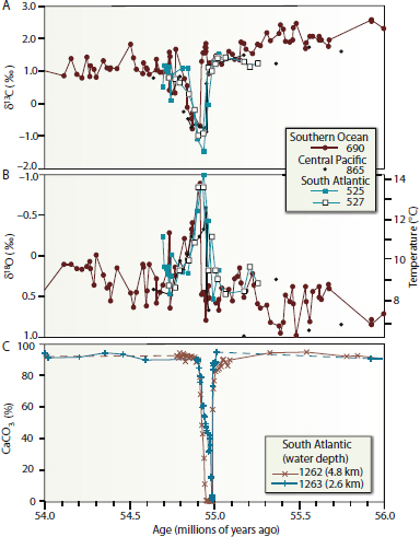
FIGURE 3.3 Marine stable isotope and seafloor sediment CaCO3 records compiled using several ocean drilling sites for the PETM, a hyperthermal with some parallels to modern greenhouse gas-driven global change. (A) δ13C time series developed from benthic foraminifera illustrating ~2.5 part per thousand (‰) excursion at ~55 Ma. (B) δ18O time series and inferred temperatures record the prolonged period of ocean warming (~70-80 ky) and its large magnitude. There may have been several events of greenhouse gas release during the PETM that produced the large, abrupt changes in ocean temperatures. (C) Record of seafloor calcium carbonate content from the South Atlantic documents the significant reduction due to dissolution and deep-ocean acidification during the PETM. The apparent onset of CaCO3 dissolution prior to the onset of the carbon isotope excursion reflects the extensive dissolution of uppermost Paleocene sediments by acidic waters during the PETM.
SOURCE: Zachos et al. (2008), reprinted by permission of Macmillan Publishers Ltd.
putative cometary particles were actually produced by bacteria (Kopp et al., 2007; Lippert and Zachos, 2007; Schumann et al., 2008). Clearly, there is no single fully satisfactory source to account for the carbon, and multiple carbon releases may have occurred in response to an initial warming. A likely trigger for the initial warming during the PETM is igneous intrusion into organic-rich sediments of the North Atlantic, which generated thermogenic methane and CO2 (Svensen et al., 2004; Storey et al., 2007). Notably, the sudden release of carbon into the atmosphere-ocean system occurred at rates that vastly exceeded typical rates in Earth history, activating components of the climate system that can be triggered by accelerated warming. The PETM serves as an important base level showing the effect on the biosphere of a rapid rate of addition of fossil carbon to the atmosphere (~3,000 to 4,500 Pg—on the order of that anticipated if we burn through all fossil fuels)—yet dwarfed by the present rate of ~1 percent per year CO2 increase in Earth’s atmosphere (Zeebe et al., 2009).
Transient warming episodes, such as the PETM, were a recurring phenomenon of the early Eocene warm world. Many of the short-lived hyperthermals were associated with abrupt and extreme climate change, an accelerated hydrological cycle, and ocean acidification (Nicolo et al., 2007; Stap et al., 2009) (Box 3.3). Short-term positive feedbacks active during the hyperthermals magnified the climatic effects of the initial carbon influx. Climate amelioration with each transient warming event would have been substantially delayed as the rates of short-term feedbacks far outpaced the negative feedbacks (e.g., weathering) capable of restoring the global carbon cycle to a steady state (Zachos et al., 2008; Zeebe et al., 2009).
The PETM, and other hyperthermals of the early Cenozoic, occurred when the Earth was virtually ice-free. This is certainly significantly different from modern and near-future conditions, which are expected to maintain unipolar glaciation at a minimum. The ice sheets of the Neoproterozoic Snowball Earth and the Late Paleozoic Ice Age were far more extensive than those of the Cenozoic icehouse, recording repeated major glacial-interglacial transitions and including terminal epic deglaciation. Despite substantially different land mass-height distributions, ocean circulation patterns, and marine and terrestrial ecosystems from those of today, the geological record of these deglaciations—specifically the repeated major transitions between glaciations and glacial minima including their terminal epic deglaciations—provide the only “icehouse” perspective of the response of the climate system and ecosystems to perturbation beyond the range archived in the more recent glacial records.
The Late Paleozoic Deglaciation
Much of the scientific understanding of feedbacks and thresholds in the current glacial climate system, and their influence on the biosphere,
BOX 3.3 Deep-Time Insights into Ocean Acidification
The early Cenozoic hyperthermals, and in particular the PETM, provide a natural laboratory to study climate sensitivity to pCO2, the interplay of short- and long-term feedbacks in the climate system, and ocean acidification under magnitudes of atmospheric pCO2 increases that are comparable to present and projected future increases. Clear evidence of deep-ocean acidification exists for the PETM (Zachos et al., 2005; Zeebe and Zachos, 2007), with corrosive waters completely dissolving calcium carbonate on the Atlantic seafloor at water depths below 2.5 km; today, this calcium carbonate compensation depth (CCD) occurs below 4 km in most ocean basins.
Whether surface waters became undersaturated is less clear since carbonate producers such as planktonic foraminifera and coccolithophorids persisted during the event. However, whereas shallow water reefs composed of corals, calcareous red and green algae, and larger benthic foraminifera were abundant prior to the PETM, metazoan reefs nearly vanished between 56 million and 55 million years ago (Scheibner and Speijer, 2008; Kiessling and Simpson, 2010). Widespread coral reefs did not reappear until the middle Eocene, at ~49 Ma. It appears that a combination of persistent warming from the late Paleocene to early Eocene, punctuated by deep-ocean acidification at the PETM, defined a threshold for coral-algal reefs that led to rapid loss and only gradual recovery. Notably, the lack of evidence for surface water acidification probably indicates that the rate of carbon addition was slower—perhaps by an order of magnitude—than projected fossil fuel emission rates under the least optimistic scenarios for the future (e.g., the A1 family of scenarios considered by IPCC [2007]) which, in box models, generates surface and deep-water acidification (Zeebe et al., 2008, 2009).
Over the past two centuries, the ocean has absorbed 40 percent of anthropogenic CO2 emissions (Zeebe et al., 2008). If fossil fuel emissions continue unabated and minimal development is put into carbon sequestration technologies, by the time humans burn through estimated fossil fuel reserves (at ~A.D. 2300 to A.D. 2400), ~5,000 gigatonnes of carbon will have been released to the atmosphere (Zachos et al., 2008). Because the rate of anthropogenic carbon input to the atmosphere greatly exceeds the mixing time of the oceans (1,000-1,500 years), CO2 will build up in the atmosphere (perhaps to ~2,000 ppmv) and the surface ocean (Kump, 2002; Zachos et al., 2008). What could be in store for this millennium? As the ocean continues to absorb CO2, carbonate ion (CO32–) concentration will fall leading to decreases in surface water pH and saturation states, a condition that is already apparent and will continue over the next century (Figure 3.4). Acidic surface waters are expected to massively affect ocean ecosystems, including the widespread loss of coral reefs. With time, acidic
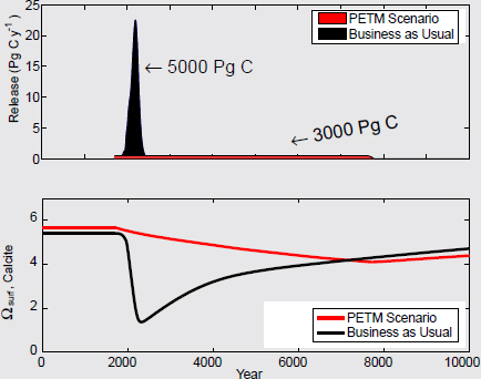
FIGURE 3.4 Initial carbon pulse for the PETM (red curves), estimated to be 3,000 Pg carbon using published carbon isotope and observed deep-sea carbonate dissolution records, and a carbon cycle model (LOSCAR; Zeebe et al., 2008, 2009). The magnitude of the input carbon mass was inferred from carbonate dissolution records, with the δ13C of the carbon pulse (≤ –50‰) constrained by requiring the model outcome to match observed deep-sea δ13C records. The model assumes a large initial input of carbon over 5 ky, followed by further smaller pulses and a low continuous carbon release (an additional 1,500 Pg) throughout the PETM main event. Changes in calcite saturation in the surface ocean (lower diagram) are estimated for the PETM (red curve) and for the future (black curve), based on the inferred magnitude of the carbon pulse to atmosphere.
SOURCE: Courtesy of R.E. Zeebe, personal communication (2010).
water will penetrate to the deep ocean where it will dissolve carbonate sediments and begin to be neutralized. In response, the saturation horizon of the deep ocean will shoal on a decadally observable timescale. Calcification rates of corals will slow noticeably and may become negligible in the next 100-150 years. At first, the rise in the saturation horizon will be slow, but as the area of seafloor above the saturation horizon declines (following the seafloor hypsometric curve), the shoaling rate will accelerate, bringing it to as shallow as the depth of the shelf-slope break (~130 m) in the next several centuries. At this point, barrier reefs, having long since lost their reef-building biota, will erode through dissolution and disintegrate. This history of carbonate dissolution will result in a carbonate-poor layer in the deep ocean, much like sediments associated with past hyperthermals such as the early Cenozoic PETM.
has been elucidated by studies of climate transitions of the past few million years—in particular the moderate-scale glacial-interglacial fluctuations of the Pleistocene. The demise of the Late Paleozoic Ice Age (LPIA; between 290 and 260 Ma) provides an opportunity to evaluate climate stability and climate-biota interactions during a major climate transition coupled to changing CO2 contents. For example, climate models indicate that climate-driven biome changes at high latitudes may have factored strongly in controlling LPIA glacial-interglacial changes (e.g., Horton et al., 2010). For the final stages of this protracted ice age, covariance between shifts in pCO2 and continental and marine surface temperatures inferred from isotopic proxies of soil-formed minerals and marine fossil brachiopods, and ice sheet extent reconstructed from southern Gondwanan glacigenic deposits, indicates a strong linkage of pCO2-climate-ice-mass dynamics that is consistent with greenhouse gas forcing (Montañez et al., 2007). A pattern of progressively more extensive and long-lived ice sheets through the Late Carboniferous (340 to 310 Ma; Fielding et al., 2008) was reversed in the Early Permian—under rising atmospheric CO2 levels—as climate ameliorated and conditions shifted toward a protracted greenhouse climate state (Montañez et al., 2007). The trend of gradually increasing surface temperatures and increasing atmospheric pCO2 is punctuated by larger but shorter-term fluctuations associated with each discrete glaciation. Surface temperatures and CO2 levels never returned to the earliest Permian minima associated with the apex of Gondwanan continental ice sheets. Intermittent warmings—characterized by CO2 levels
above the simulated threshold for glaciation (Horton et al., 2007; Horton and Poulsen, 2009)—heralded the more permanent change to an ice-free world to come. This pattern of episodic changes in atmospheric CO2 and surface temperatures in step with transient glaciations, superimposed on a longer-term warming trend during the demise of the Late Paleozoic Ice Age, shares characteristics in common with the Eocene-Oligocene greenhouse-to-icehouse transition (Coxall et al., 2005; Liu et al., 2009a,b). The similarity in behavior of these very different transitions suggests that turnovers in climate states are most probably characterized by large-scale episodic change. Future study of the deep-time record of the Earth’s last epic deglaciation should shed light on how the cryosphere, hydrosphere, chemosphere, and biosphere responded to such episodic change under rising CO2 levels.
Deglaciation During the Neoproterozoic
A phase of rapid global warming is recorded in the late Neoproterozoic (~635 Ma), abruptly terminating what was probably the longest-lived (~135 Ma; Macdonald et al., 2010) and coldest icehouse period of Earth history, where at times ice sheets extended to sea level in equatorial latitudes—a climate state popularly referred to as the “Snowball Earth” (Hoffman et al., 1998). Carbon isotope trends provide evidence for substantial, but poorly understood, disruption of the carbon cycle during the ice age itself, including the possibility that the high albedo of a global-scale ice sheet dominated climate (Hoffman et al., 1998). The terminal deglaciation in the Neoproterozoic offers an intriguing deep-time archive of how major changes in long-term processes that regulate climate, such as silicate weathering and carbon burial and productivity, have been triggered when a threshold in the climate system has been reached through CO2 forcing. Abrupt and rapid increase in CO2 at the end of the Neoproterozoic glaciations is recorded by the presence of thin calcium carbonate deposits, interpreted to have been deposited on a millennial timescale, immediately overlying Neoproterozoic glacial sediments across the globe (Kennedy et al., 1998; Hoffman and Schrag, 2002). These carbonate deposits are a physical record of rapid release of CO2 to the atmosphere calculated at a rate of ~1 percent CO2 increase per year (Kennedy et al., 2001), similar to the current rate of CO2 increase of 0.8 to 1 percent per year (IPCC, 2007). While the analogy is imperfect because of the very different biosphere and continental configuration in the Neoproterozoic, deglaciation under this strong greenhouse gas forcing imparted a record unique from that of subsequent deglaciations. Most notably, the abrupt transition to greenhouse conditions associated with this complete deglaciation appears to have involved a dominating rapid-warming feedback (Fairchild and Kennedy, 2007) that
involved the massive release of CO2 (Hoffman and Schrag, 2002) and/or the destabilization of methane clathrates and the release of methane gas from permafrost and marine reservoirs (Kennedy et al., 2001, 2009). It appears that the dominance by warming feedbacks during the termination of this ice age precluded the damping effects of other feedbacks that governed climate oscillations during Phanerozoic ice ages. Consequently, the late Neoproterozoic deglaciation provides an excellent example of the long-term feedbacks that can be triggered—and likely accelerated—when a threshold in a strongly forced climate system is reached.
HOW LONG WILL THE GREENHOUSE LAST?
The potential for climatic consequences with severe impact on humans resulting from the buildup of fossil fuel CO2 has inevitably resulted in questions not only of “How bad will it get and how fast?” but also “How long will it last?” The answers to these questions depend heavily on the global warming potential of the greenhouse gas release, which accounts not only for its immediate impact on the planetary radiative energy balance but also on the longevity of the greenhouse gas in the atmosphere (Archer et al., 2009).
Economic forecasts suggest that conventional fossil fuel resources will largely be used up in the next 200-400 years, leading to atmospheric CO2 levels that could reach ~2,000 ppmv by A.D. 2300 to 2400 (Marland et al., 2002; Caldeira and Wickett, 2003). However, models of the global carbon cycle and the geologic record both show that CO2 produced from fossil fuels and other reservoirs will continue to impact global climate and atmospheric chemistry for tens to hundreds of thousands of years. Although CO2 produced by fossil fuel burning is taken out of the atmosphere within decades of its production, the oceans, soils, and vegetation continue to exchange greenhouse gases back into the atmosphere for far longer. Greenhouse gases continue to affect climate and ocean acidity until they are buried as organic matter or converted to mineral forms of inorganic carbon through rock weathering (Box 3.4).
Simple box models (Figure 3.6) have been used to make long-term projections of future climate to capture the “recovery” from the fossil fuel-induced greenhouse state (Walker and Kasting, 1992; Archer, 2005). Although box model calculations should not be considered definitive, they do suggest that the fossil fuel perturbation may interfere with the natural glacial-interglacial oscillation driven by predictable changes in Earth’s orbit (Berger et al., 2003), perhaps forestalling the onset of the next northern hemisphere “ice age” by tens of thousands of years. A more convincing exposition of the central question of “how long” requires more comprehensive models. Scientific confidence in those models will be high
BOX 3.4 CO2 Sweepers and Sinks in the Earth System
The carbon fluxes in and out of the surface and sedimentary reservoirs over geological timescales are finely balanced, providing a planetary thermostat that regulates Earth’s surface temperature. Initially, newly released CO2 (e.g., from the combustion of hydrocarbons) interacts and equilibrates with Earth’s surface reservoirs of carbon on human timescales (decades to centuries). However, natural “sinks” for anthropogenic CO2 exist only on much longer timescales, and it is therefore possible to perturb climate for tens to hundreds of thousands of years (Figure 3.5). Transient (annual to century-scale) uptake by the terrestrial biosphere (including soils) is easily saturated within decades of the CO2 increase, and therefore this component can switch from a sink to a source of atmospheric CO2 (Friedlingstein et al., 2006). Most (60 to 80 percent) CO2 is ultimately absorbed by the surface ocean, because of its efficiency as a sweeper of atmospheric CO2, and is neutralized by reactions with calcium carbonate in the deep sea at timescales of oceanic mixing (1,000 to 1,500 years). The ocean’s ability to sequester CO2 decreases as it is acidified and the oceanic carbon buffer is depleted. The remaining CO2 in the atmosphere is sufficient to impact climate for thousands of years longer while awaiting sweeping by the “ultimate” CO2 sink of the rock weathering cycle at timescales of tens to hundreds of thousands of years (Zeebe and Caldeira, 2008; Archer et al., 2009). Lessons from past hyperthermals suggest that the removal of greenhouse gases by weathering may be intensified in a warmer world but will still take more than 100,000 years to return to background values for an event the size of the Paleocene-Eocene Thermal Maximum.
In the context of the timescales of interaction with these carbon sinks, the mean lifetime of fossil fuel CO2 in the atmosphere is calculated to be 12,000 to 14,000 years (Archer et al., 1997, 2009), which is in marked contrast to the two to three orders of magnitude shorter lifetimes commonly cited by other studies (e.g., IPCC, 1995, 2001). In addition, the equilibration timescale for a pulse of CO2 emission to the atmosphere, such as the current release by fossil fuel burning, scales up with the magnitude of the CO2 release. “The result has been an erroneous conclusion, throughout much of the popular treatment of the issue of climate change, that global warming will be a century-timescale phenomenon” (Archer et al., 2009, p. 121).
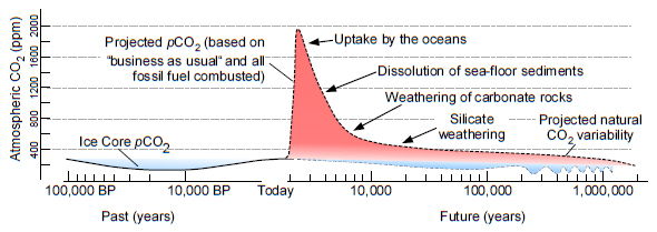
FIGURE 3.5 Graphic portrayal of the CO2 “lifetime” assuming nonlinear CO2 uptake kinetics by various short (decades to millennia) and long-term (104 to 105 y) surface and sedimentary carbon reservoirs. Projected natural CO2 variability assumes 100 ky orbital control.
SOURCE: Modified from Walker and Kasting (1992); B.B. Sageman, personal communication.
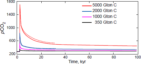
FIGURE 3.6 Schematic showing the predicted long-term response over 100,000 years of atmospheric CO2, including ocean temperature feedbacks, to a range of possible fossil fuel emissions totals. The 100,000-year simulations include silicate weathering (solid lines) and the 35,000-year simulations include seafloor CaCO3 dissolution (dashed lines). These models highlight how the timescale of carbon uptake becomes extended as the event unfolds. Fast processes such as ocean uptake and biomass growth, with high transfer rates but limited capacity, lose their potency, while slower processes, such as seafloor carbonate dissolution and rock weathering, come to dominate.
SOURCE: Modified from Archer (2005).
only if they can be evaluated against observation. The historical record, and even the expanse of the Quaternary climate record, contains nothing comparable.
Observations and modeling of the past carbon cycle perturbations provide a basis for projecting future conditions under the full range of fossil fuel burning scenarios, including the most pessimistic “business-as-usual” eventuality. Along this trajectory, atmospheric CO2 levels will rise as long as fossil fuel burning continues (with ultimate input of ~5,000 GtC), rising to levels perhaps as high as 1,600-2,000 parts per million (i.e., five to seven times the preindustrial level) (Figure 3.6). The geological record of past hyperthermal events, including the PETM, suggests that severe global warming under such magnitudes of carbon emissions will persist for 20,000 to 40,000 years. Carbon cycle models indicate that even after 100,000 years, the anthropogenic perturbation to the carbon cycle will still be important, especially if the total amount of carbon emitted is large. Consequently, Milankovitch forcings that have so dominated the pacing and extent of climate variations, and especially ice sheets, over the last 2 million years will—as they were prior to the onset of the current
glacial state in the Oligocene—serve as only a minor modulator of high-latitude climate variability because climate change will be muted under such elevated atmospheric pCO2 levels. The Greenland ice cap could disappear in the first few coming millennia, and if CO2 levels rise more than two to four times present levels, the West Antarctic ice cap could collapse (Naish et al., 2009), although this conclusion is highly sensitive to orbital configuration and model parameterizations (Pollard and DeConto, 2005). By any measure, exploitation of much of the fossil fuel reservoir over only 300 years will clearly leave a far longer lasting legacy.


