
Reference Guide on Multiple Regression
Daniel L. Rubinfeld, Ph.D., is Robert L. Bridges Professor of Law and Professor of Economics Emeritus, University of California, Berkeley, and Visiting Professor of Law at New York University Law School.
CONTENTS
II. Research Design: Model Specification
A. What Is the Specific Question That Is Under Investigation by the Expert?
B. What Model Should Be Used to Evaluate the Question at Issue?
1. Choosing the dependent variable
2. Choosing the explanatory variable that is relevant to the question at issue
3. Choosing the additional explanatory variables
4. Choosing the functional form of the multiple regression model
5. Choosing multiple regression as a method of analysis
III. Interpreting Multiple Regression Results
A. What Is the Practical, as Opposed to the Statistical, Significance of Regression Results?
1. When should statistical tests be used?
2. What is the appropriate level of statistical significance?
3. Should statistical tests be one-tailed or two-tailed?
B. Are the Regression Results Robust?
1. What evidence exists that the explanatory variable causes changes in the dependent variable?
2. To what extent are the explanatory variables correlated with each other?
3. To what extent are individual errors in the regression model independent?
4. To what extent are the regression results sensitive to individual data points?
5. To what extent are the data subject to measurement error?
A. Who Should Be Qualified as an Expert?
B. Should the Court Appoint a Neutral Expert?
V. Presentation of Statistical Evidence
A. What Disagreements Exist Regarding Data on Which the Analysis Is Based?
Appendix: The Basics of Multiple Regression
1. Specifying the regression model
C. Interpreting Regression Results
D. Determining the Precision of the Regression Results
1. Standard errors of the coefficients and t-statistics
3. Sensitivity of least squares regression results
Multiple regression analysis is a statistical tool used to understand the relationship between or among two or more variables.1 Multiple regression involves a variable to be explained—called the dependent variable—and additional explanatory variables that are thought to produce or be associated with changes in the dependent variable.2 For example, a multiple regression analysis might estimate the effect of the number of years of work on salary. Salary would be the dependent variable to be explained; the years of experience would be the explanatory variable.
Multiple regression analysis is sometimes well suited to the analysis of data about competing theories for which there are several possible explanations for the relationships among a number of explanatory variables.3 Multiple regression typically uses a single dependent variable and several explanatory variables to assess the statistical data pertinent to these theories. In a case alleging sex discrimination in salaries, for example, a multiple regression analysis would examine not only sex, but also other explanatory variables of interest, such as education and experience.4 The employer-defendant might use multiple regression to argue that salary is a function of the employee’s education and experience, and the employee-plaintiff might argue that salary is also a function of the individual’s sex. Alternatively, in an antitrust cartel damages case, the plaintiff’s expert might utilize multiple regression to evaluate the extent to which the price of a product increased during the period in which the cartel was effective, after accounting for costs and other variables unrelated to the cartel. The defendant’s expert might use multiple
1. A variable is anything that can take on two or more values (e.g., the daily temperature in Chicago or the salaries of workers at a factory).
2. Explanatory variables in the context of a statistical study are sometimes called independent variables. See David H. Kaye & David A. Freedman, Reference Guide on Statistics, Section II.A.1, in this manual. The guide also offers a brief discussion of multiple regression analysis. Id., Section V.
3. Multiple regression is one type of statistical analysis involving several variables. Other types include matching analysis, stratification, analysis of variance, probit analysis, logit analysis, discriminant analysis, and factor analysis.
4. Thus, in Ottaviani v. State University of New York, 875 F.2d 365, 367 (2d Cir. 1989) (citations omitted), cert. denied, 493 U.S. 1021 (1990), the court stated:
In disparate treatment cases involving claims of gender discrimination, plaintiffs typically use multiple regression analysis to isolate the influence of gender on employment decisions relating to a particular job or job benefit, such as salary.
The first step in such a regression analysis is to specify all of the possible “legitimate” (i.e., nondiscriminatory) factors that are likely to significantly affect the dependent variable and which could account for disparities in the treatment of male and female employees. By identifying those legitimate criteria that affect the decisionmaking process, individual plaintiffs can make predictions about what job or job benefits similarly situated employees should ideally receive, and then can measure the difference between the predicted treatment and the actual treatment of those employees. If there is a disparity between the predicted and actual outcomes for female employees, plaintiffs in a disparate treatment case can argue that the net “residual” difference represents the unlawful effect of discriminatory animus on the allocation of jobs or job benefits.
regression to suggest that the plaintiff’s expert had omitted a number of price-determining variables.
More generally, multiple regression may be useful (1) in determining whether a particular effect is present; (2) in measuring the magnitude of a particular effect; and (3) in forecasting what a particular effect would be, but for an intervening event. In a patent infringement case, for example, a multiple regression analysis could be used to determine (1) whether the behavior of the alleged infringer affected the price of the patented product, (2) the size of the effect, and (3) what the price of the product would have been had the alleged infringement not occurred.
Over the past several decades, the use of multiple regression analysis in court has grown widely. Regression analysis has been used most frequently in cases of sex and race discrimination5 antitrust violations,6 and cases involving class cer-
5. Discrimination cases using multiple regression analysis are legion. See, e.g., Bazemore v. Friday, 478 U.S. 385 (1986), on remand, 848 F.2d 476 (4th Cir. 1988); Csicseri v. Bowsher, 862 F. Supp. 547 (D.D.C. 1994) (age discrimination), aff’d, 67 F.3d 972 (D.C. Cir. 1995); EEOC v. General Tel. Co., 885 F.2d 575 (9th Cir. 1989), cert. denied, 498 U.S. 950 (1990); Bridgeport Guardians, Inc. v. City of Bridgeport, 735 F. Supp. 1126 (D. Conn. 1990), aff’d, 933 F.2d 1140 (2d Cir.), cert. denied, 502 U.S. 924 (1991); Bickerstaff v. Vassar College, 196 F.3d 435, 448–49 (2d Cir. 1999) (sex discrimination); McReynolds v. Sodexho Marriott, 349 F. Supp. 2d 1 (D.C. Cir. 2004) (race discrimination); Hnot v. Willis Group Holdings Ltd., 228 F.R.D. 476 (S.D.N.Y. 2005) (gender discrimination); Carpenter v. Boeing Co., 456 F.3d 1183 (10th Cir. 2006) (sex discrimination); Coward v. ADT Security Systems, Inc., 140 F.3d 271, 274–75 (D.C. Cir. 1998); Smith v. Virginia Commonwealth Univ., 84 F.3d 672 (4th Cir. 1996) (en banc); Hemmings v. Tidyman’s Inc., 285 F.3d 1174, 1184–86 (9th Cir. 2000); Mehus v. Emporia State University, 222 F.R.D. 455 (D. Kan. 2004) (sex discrimination); Guiterrez v. Johnson & Johnson, 2006 WL 3246605 (D.N.J. Nov. 6, 2006 (race discrimination); Morgan v. United Parcel Service, 380 F.3d 459 (8th Cir. 2004) (racial discrimination). See also Keith N. Hylton & Vincent D. Rougeau, Lending Discrimination: Economic Theory, Econometric Evidence, and the Community Reinvestment Act, 85 Geo. L.J. 237, 238 (1996) (“regression analysis is probably the best empirical tool for uncovering discrimination”).
6. E.g., United States v. Brown Univ., 805 F. Supp. 288 (E.D. Pa. 1992) (price fixing of college scholarships), rev’d, 5 F.3d 658 (3d Cir. 1993); Petruzzi’s IGA Supermarkets, Inc. v. Darling-Delaware Co., 998 F.2d 1224 (3d Cir.), cert. denied, 510 U.S. 994 (1993); Ohio v. Louis Trauth Dairy, Inc., 925 F. Supp. 1247 (S.D. Ohio 1996); In re Chicken Antitrust Litig., 560 F. Supp. 963, 993 (N.D. Ga. 1980); New York v. Kraft Gen. Foods, Inc., 926 F. Supp. 321 (S.D.N.Y. 1995); Freeland v. AT&T, 238 F.R.D. 130 (S.D.N.Y. 2006); In re Pressure Sensitive Labelstock Antitrust Litig., 2007 U.S. Dist. LEXIS 85466 (M.D. Pa. Nov. 19, 2007); In re Linerboard Antitrust Litig., 497 F. Supp. 2d 666 (E.D. Pa. 2007) (price fixing by manufacturers of corrugated boards and boxes); In re Polypropylene Carpet Antitrust Litig., 93 F. Supp. 2d 1348 (N.D. Ga. 2000); In re OSB Antitrust Litig., 2007 WL 2253418 (E.D. Pa. Aug. 3, 2007) (price fixing of Oriented Strand Board, also known as “waferboard”); In re TFT-LCD (Flat Panel) Antitrust Litig., 267 F.R.D. 583 (N.D. Cal. 2010).
For a broad overview of the use of regression methods in antitrust, see ABA Antitrust Section, Econometrics: Legal, Practical and Technical Issues (John Harkrider & Daniel Rubinfeld, eds. 2005). See also Jerry Hausman et al., Competitive Analysis with Differenciated Products, 34 Annales D’Économie et de Statistique 159 (1994); Gregory J. Werden, Simulating the Effects of Differentiated Products Mergers: A Practical Alternative to Structural Merger Policy, 5 Geo. Mason L. Rev. 363 (1997).
tification (under Rule 23).7 However, there are a range of other applications, including census undercounts,8 voting rights,9 the study of the deterrent effect of the death penalty,10 rate regulation,11 and intellectual property.12
7. In antitrust, the circuits are currently split as to the extent to which plaintiffs must prove that common elements predominate over individual elements. E.g., compare In Re Hydrogen Peroxide Litig., 522 F.2d 305 (3d Cir. 2008) with In Re Cardizem CD Antitrust Litig., 391 F.3d 812 (6th Cir. 2004). For a discussion of use of multiple regression in evaluating class certification, see Bret M. Dickey & Daniel L. Rubinfeld, Antitrust Class Certification: Towards an Economic Framework, 66 N.Y.U. Ann. Surv. Am. L. 459 (2010) and John H. Johnson & Gregory K. Leonard, Economics and the Rigorous Analysis of Class Certification in Antitrust Cases, 3 J. Competition L. & Econ. 341 (2007).
8. See, e.g., City of New York v. U.S. Dep’t of Commerce, 822 F. Supp. 906 (E.D.N.Y. 1993) (decision of Secretary of Commerce not to adjust the 1990 census was not arbitrary and capricious), vacated, 34 F.3d 1114 (2d Cir. 1994) (applying heightened scrutiny), rev’d sub nom. Wisconsin v. City of New York, 517 U.S. 565 (1996); Carey v. Klutznick, 508 F. Supp. 420, 432–33 (S.D.N.Y. 1980) (use of reasonable and scientifically valid statistical survey or sampling procedures to adjust census figures for the differential undercount is constitutionally permissible), stay granted, 449 U.S. 1068 (1980), rev’d on other grounds, 653 F.2d 732 (2d Cir. 1981), cert. denied, 455 U.S. 999 (1982); Young v. Klutznick, 497 F. Supp. 1318, 1331 (E.D. Mich. 1980), rev’d on other grounds, 652 F.2d 617 (6th Cir. 1981), cert. denied, 455 U.S. 939 (1982).
9. Multiple regression analysis was used in suits charging that at-large areawide voting was instituted to neutralize black voting strength, in violation of section 2 of the Voting Rights Act, 42 U.S.C. § 1973 (1988). Multiple regression demonstrated that the race of the candidates and that of the electorate were determinants of voting. See Williams v. Brown, 446 U.S. 236 (1980); Rodriguez v. Pataki, 308 F. Supp. 2d 346, 414 (S.D.N.Y. 2004); United States v. Vill. of Port Chester, 2008 U.S. Dist. LEXIS 4914 (S.D.N.Y. Jan. 17, 2008); Meza v. Galvin, 322 F. Supp. 2d 52 (D. Mass. 2004) (violation of VRA with regard to Hispanic voters in Boston); Bone Shirt v. Hazeltine, 336 F. Supp. 2d 976 (D.S.D. 2004) (violations of VRA with regard to Native American voters in South Dakota); Georgia v. Ashcroft, 195 F. Supp. 2d 25 (D.D.C. 2002) (redistricting of Georgia’s state and federal legislative districts); Benavidez v. City of Irving, 638 F. Supp. 2d 709 (N.D. Tex. 2009) (challenge of city’s at-large voting scheme). For commentary on statistical issues in voting rights cases, see, e.g., Statistical and Demographic Issues Underlying Voting Rights Cases, 15 Evaluation Rev. 659 (1991); Stephen P. Klein et al., Ecological Regression Versus the Secret Ballot, 31 Jurimetrics J. 393 (1991); James W. Loewen & Bernard Grofman, Recent Developments in Methods Used in Vote Dilution Litigation, 21 Urb. Law. 589 (1989); Arthur Lupia & Kenneth McCue, Why the 1980s Measures of Racially Polarized Voting Are Inadequate for the 1990s, 12 Law & Pol’y 353 (1990).
10. See, e.g., Gregg v. Georgia, 428 U.S. 153, 184–86 (1976). For critiques of the validity of the deterrence analysis, see National Research Council, Deterrence and Incapacitation: Estimating the Effects of Criminal Sanctions on Crime Rates (Alfred Blumstein et al. eds., 1978); Richard O. Lempert, Desert and Deterrence: An Assessment of the Moral Bases of the Case for Capital Punishment, 79 Mich. L. Rev. 1177 (1981); Hans Zeisel, The Deterrent Effect of the Death Penalty: Facts v. Faith, 1976 Sup. Ct. Rev. 317; and John Donohue & Justin Wolfers, Uses and Abuses of Statistical Evidence in the Death Penalty Debate, 58 Stan. L. Rev. 787 (2005).
11. See, e.g., Time Warner Entertainment Co. v. FCC, 56 F.3d 151 (D.C. Cir. 1995) (challenge to FCC’s application of multiple regression analysis to set cable rates), cert. denied, 516 U.S. 1112 (1996); Appalachian Power Co. v. EPA, 135 F.3d 791 (D.C. Cir. 1998) (challenging the EPA’s application of regression analysis to set nitrous oxide emission limits); Consumers Util. Rate Advocacy Div. v. Ark. PSC, 99 Ark. App. 228 (Ark. Ct. App. 2007) (challenging an increase in nongas rates).
12. See Polaroid Corp. v. Eastman Kodak Co., No. 76-1634-MA, 1990 WL 324105, at *29, *62–63 (D. Mass. Oct. 12, 1990) (damages awarded because of patent infringement), amended by No.
Multiple regression analysis can be a source of valuable scientific testimony in litigation. However, when inappropriately used, regression analysis can confuse important issues while having little, if any, probative value. In EEOC v. Sears, Roebuck & Co.,13 in which Sears was charged with discrimination against women in hiring practices, the Seventh Circuit acknowledged that “[m]ultiple regression analyses, designed to determine the effect of several independent variables on a dependent variable, which in this case is hiring, are an accepted and common method of proving disparate treatment claims.”14 However, the court affirmed the district court’s findings that the “E.E.O.C.’s regression analyses did not ‘accurately reflect Sears’ complex, nondiscriminatory decision-making processes’” and that the “‘E.E.O.C.’s statistical analyses [were] so flawed that they lack[ed] any persuasive value.’”15 Serious questions also have been raised about the use of multiple regression analysis in census undercount cases and in death penalty cases.16
The Supreme Court’s rulings in Daubert and Kumho Tire have encouraged parties to raise questions about the admissibility of multiple regression analyses.17 Because multiple regression is a well-accepted scientific methodology, courts have frequently admitted testimony based on multiple regression studies, in some cases over the strong objection of one of the parties.18 However, on some occasions courts have excluded expert testimony because of a failure to utilize a multiple regression methodology.19 On other occasions, courts have rejected regression
76-1634-MA, 1991 WL 4087 (D. Mass. Jan. 11, 1991); Estate of Vane v. The Fair, Inc., 849 F.2d 186, 188 (5th Cir. 1988) (lost profits were the result of copyright infringement), cert. denied, 488 U.S. 1008 (1989); Louis Vuitton Malletier v. Dooney & Bourke, Inc., 525 F. Supp. 2d 576, 664 (S.D.N.Y. 2007) (trademark infringement and unfair competition suit). The use of multiple regression analysis to estimate damages has been contemplated in a wide variety of contexts. See, e.g., David Baldus et al., Improving Judicial Oversight of Jury Damages Assessments: A Proposal for the Comparative Additur/Remittitur Review of Awards for Nonpecuniary Harms and Punitive Damages, 80 Iowa L. Rev. 1109 (1995); Talcott J. Franklin, Calculating Damages for Loss of Parental Nurture Through Multiple Regression Analysis, 52 Wash. & Lee L. Rev. 271 (1997); Roger D. Blair & Amanda Kay Esquibel, Yardstick Damages in Lost Profit Cases: An Econometric Approach, 72 Denv. U. L. Rev. 113 (1994). Daniel Rubinfeld, Quantitative Methods in Antitrust, in 1 Issues in Competition Law and Policy 723 (2008).
13. 839 F.2d 302 (7th Cir. 1988).
14. Id. at 324 n.22.
15. Id. at 348, 351 (quoting EEOC v. Sears, Roebuck & Co., 628 F. Supp. 1264, 1342, 1352 (N.D. Ill. 1986)). The district court commented specifically on the “severe limits of regression analysis in evaluating complex decision-making processes.” 628 F. Supp. at 1350.
16. See David H. Kaye & David A. Freedman, Reference Guide on Statistics, Sections II.A.3, B.1, in this manual.
17. Daubert v. Merrill Dow Pharms., Inc. 509 U.S. 579 (1993); Kumho Tire Co. v. Carmichael, 526 U.S. 137, 147 (1999) (expanding the Daubert’s application to nonscientific expert testimony).
18. See Newport Ltd. v. Sears, Roebuck & Co., 1995 U.S. Dist. LEXIS 7652 (E.D. La. May 26, 1995). See also Petruzzi’s IGA Supermarkets, supra note 6, 998 F.2d at 1240, 1247 (finding that the district court abused its discretion in excluding multiple regression-based testimony and reversing the grant of summary judgment to two defendants).
19. See, e.g., In re Executive Telecard Ltd. Sec. Litig., 979 F. Supp. 1021 (S.D.N.Y. 1997).
studies that did not have an adequate foundation or research design with respect to the issues at hand.20
In interpreting the results of a multiple regression analysis, it is important to distinguish between correlation and causality. Two variables are correlated—that is, associated with each other—when the events associated with the variables occur more frequently together than one would expect by chance. For example, if higher salaries are associated with a greater number of years of work experience, and lower salaries are associated with fewer years of experience, there is a positive correlation between salary and number of years of work experience. However, if higher salaries are associated with less experience, and lower salaries are associated with more experience, there is a negative correlation between the two variables.
A correlation between two variables does not imply that one event causes the second. Therefore, in making causal inferences, it is important to avoid spurious correlation.21 Spurious correlation arises when two variables are closely related but bear no causal relationship because they are both caused by a third, unexamined variable. For example, there might be a negative correlation between the age of certain skilled employees of a computer company and their salaries. One should not conclude from this correlation that the employer has necessarily discriminated against the employees on the basis of their age. A third, unexamined variable, such as the level of the employees’ technological skills, could explain differences in productivity and, consequently, differences in salary.22 Or, consider a patent infringement case in which increased sales of an allegedly infringing product are associated with a lower price of the patented product.23 This correlation would be spurious if the two products have their own noncompetitive market niches and the lower price is the result of a decline in the production costs of the patented product.
Pointing to the possibility of a spurious correlation will typically not be enough to dispose of a statistical argument. It may be appropriate to give little weight to such an argument absent a showing that the correlation is relevant. For example, a statistical showing of a relationship between technological skills
20. See City of Tuscaloosa v. Harcros Chemicals, Inc., 158 F.2d 548 (11th Cir. 1998), in which the court ruled plaintiffs’ regression-based expert testimony inadmissible and granted summary judgment to the defendants. See also American Booksellers Ass’n v. Barnes & Noble, Inc., 135 F. Supp. 2d 1031, 1041 (N.D. Cal. 2001), in which a model was said to contain “too many assumptions and simplifications that are not supported by real-world evidence,” and Obrey v. Johnson, 400 F.3d 691 (9th Cir. 2005).
21. See David H. Kaye & David A. Freedman, Reference Guide on Statistics, Section V.B.3, in this manual.
22. See, e.g., Sheehan v. Daily Racing Form Inc., 104 F.3d 940, 942 (7th Cir.) (rejecting plaintiff’s age discrimination claim because statistical study showing correlation between age and retention ignored the “more than remote possibility that age was correlated with a legitimate job-related qualification”), cert. denied, 521 U.S. 1104 (1997).
23. In some particular cases, there are statistical tests that allow one to reject claims of causality. For a brief description of these tests, which were developed by Jerry Hausman, see Robert S. Pindyck & Daniel L. Rubinfeld, Econometric Models and Economic Forecasts § 7.5 (4th ed. 1997).
and worker productivity might be required in the age discrimination example, above.24
Causality cannot be inferred by data analysis alone; rather, one must infer that a causal relationship exists on the basis of an underlying causal theory that explains the relationship between the two variables. Even when an appropriate theory has been identified, causality can never be inferred directly. One must also look for empirical evidence that there is a causal relationship. Conversely, the fact that two variables are correlated does not guarantee the existence of a relationship; it could be that the model—a characterization of the underlying causal theory—does not reflect the correct interplay among the explanatory variables. In fact, the absence of correlation does not guarantee that a causal relationship does not exist. Lack of correlation could occur if (1) there are insufficient data, (2) the data are measured inaccurately, (3) the data do not allow multiple causal relationships to be sorted out, or (4) the model is specified wrongly because of the omission of a variable or variables that are related to the variable of interest.
There is a tension between any attempt to reach conclusions with near certainty and the inherently uncertain nature of multiple regression analysis. In general, the statistical analysis associated with multiple regression allows for the expression of uncertainty in terms of probabilities. The reality that statistical analysis generates probabilities concerning relationships rather than certainty should not be seen in itself as an argument against the use of statistical evidence, or worse, as a reason to not admit that there is uncertainty at all. The only alternative might be to use less reliable anecdotal evidence.
This reference guide addresses a number of procedural and methodological issues that are relevant in considering the admissibility of, and weight to be accorded to, the findings of multiple regression analyses. It also suggests some standards of reporting and analysis that an expert presenting multiple regression analyses might be expected to meet. Section II discusses research design—how the multiple regression framework can be used to sort out alternative theories about a case. The guide discusses the importance of choosing the appropriate specification of the multiple regression model and raises the issue of whether multiple regression is appropriate for the case at issue. Section III accepts the regression framework and concentrates on the interpretation of the multiple regression results from both a statistical and a practical point of view. It emphasizes the distinction between regression results that are statistically significant and results that are meaningful to the trier of fact. It also points to the importance of evaluating the robustness
24. See, e.g., Allen v. Seidman, 881 F.2d 375 (7th Cir. 1989) (judicial skepticism was raised when the defendant did not submit a logistic regression incorporating an omitted variable—the possession of a higher degree or special education; defendant’s attack on statistical comparisons must also include an analysis that demonstrates that comparisons are flawed). The appropriate requirements for the defendant’s showing of spurious correlation could, in general, depend on the discovery process. See, e.g., Boykin v. Georgia Pac. Co., 706 F.2d 1384 (1983) (criticism of a plaintiff’s analysis for not including omitted factors, when plaintiff considered all information on an application form, was inadequate).
of regression analyses, i.e., seeing the extent to which the results are sensitive to changes in the underlying assumptions of the regression model. Section IV briefly discusses the qualifications of experts and suggests a potentially useful role for court-appointed neutral experts. Section V emphasizes procedural aspects associated with use of the data underlying regression analyses. It encourages greater pretrial efforts by the parties to attempt to resolve disputes over statistical studies.
Throughout the main body of this guide, hypothetical examples are used as illustrations. Moreover, the basic “mathematics” of multiple regression has been kept to a bare minimum. To achieve that goal, the more formal description of the multiple regression framework has been placed in the Appendix. The Appendix is self-contained and can be read before or after the text. The Appendix also includes further details with respect to the examples used in the body of this guide.
II. Research Design: Model Specification
Multiple regression allows the testifying economist or other expert to choose among alternative theories or hypotheses and assists the expert in distinguishing correlations between variables that are plainly spurious from those that may reflect valid relationships.
A. What Is the Specific Question That Is Under Investigation by the Expert?
Research begins with a clear formulation of a research question. The data to be collected and analyzed must relate directly to this question; otherwise, appropriate inferences cannot be drawn from the statistical analysis. For example, if the question at issue in a patent infringement case is what price the plaintiff’s product would have been but for the sale of the defendant’s infringing product, sufficient data must be available to allow the expert to account statistically for the important factors that determine the price of the product.
B. What Model Should Be Used to Evaluate the Question at Issue?
Model specification involves several steps, each of which is fundamental to the success of the research effort. Ideally, a multiple regression analysis builds on a theory that describes the variables to be included in the study. A typical regression model will include one or more dependent variables, each of which is believed to be causally related to a series of explanatory variables. Because we cannot be certain that the explanatory variables are themselves unaffected or independent of the influence of the dependent variable (at least at the point of initial study), the explanatory
variables are often termed covariates. Covariates are known to have an association with the dependent or outcome variable, but causality remains an open question.
For example, the theory of labor markets might lead one to expect salaries in an industry to be related to workers’ experience and the productivity of workers’ jobs. A belief that there is job discrimination would lead one to create a model in which the dependent variable was a measure of workers’ salaries and the list of covariates included a variable reflecting discrimination in addition to measures of job training and experience.
In a perfect world, the analysis of the job discrimination (or any other) issue might be accomplished through a controlled “natural experiment,” in which employees would be randomly assigned to a variety of employers in an industry under study and asked to fill positions requiring identical experience and skills. In this observational study, where the only difference in salaries could be a result of discrimination, it would be possible to draw clear and direct inferences from an analysis of salary data. Unfortunately, the opportunity to conduct observational studies of this kind is rarely available to experts in the context of legal proceedings. In the real world, experts must do their best to interpret the results of real-world “quasi-experiments,” in which it is impossible to control all factors that might affect worker salaries or other variables of interest.25
Models are often characterized in terms of parameters—numerical characteristics of the model. In the labor market discrimination example, one parameter might reflect the increase in salary associated with each additional year of prior job experience. Another parameter might reflect the reduction in salary associated with a lack of current on-the-job experience. Multiple regression uses a sample, or a selection of data, from the population (all the units of interest) to obtain estimates of the values of the parameters of the model. An estimate associated with a particular explanatory variable is an estimated regression coefficient.
Failure to develop the proper theory, failure to choose the appropriate variables, or failure to choose the correct form of the model can substantially bias the statistical results—that is, create a systematic tendency for an estimate of a model parameter to be too high or too low.
1. Choosing the dependent variable
The variable to be explained, the dependent variable, should be the appropriate variable for analyzing the question at issue.26 Suppose, for example, that pay dis-
25. In the literature on natural and quasi-experiments, the explanatory variables are characterized as “treatments” and the dependent variable as the “outcome.” For a review of natural experiments in the criminal justice arena, see David P. Farrington, A Short History of Randomized Experiments in Criminology, 27 Evaluation Rev. 218–27 (2003).
26. In multiple regression analysis, the dependent variable is usually a continuous variable that takes on a range of numerical values. When the dependent variable is categorical, taking on only two or three values, modified forms of multiple regression, such as probit analysis or logit analysis, are
crimination among hourly workers is a concern. One choice for the dependent variable is the hourly wage rate of the employees; another choice is the annual salary. The distinction is important, because annual salary differences may in part result from differences in hours worked. If the number of hours worked is the product of worker preferences and not discrimination, the hourly wage is a good choice. If the number of hours worked is related to the alleged discrimination, annual salary is the more appropriate dependent variable to choose.27
2. Choosing the explanatory variable that is relevant to the question at issue
The explanatory variable that allows the evaluation of alternative hypotheses must be chosen appropriately. Thus, in a discrimination case, the variable of interest may be the race or sex of the individual. In an antitrust case, it may be a variable that takes on the value 1 to reflect the presence of the alleged anticompetitive behavior and the value 0 otherwise.28
3. Choosing the additional explanatory variables
An attempt should be made to identify additional known or hypothesized explanatory variables, some of which are measurable and may support alternative substantive hypotheses that can be accounted for by the regression analysis. Thus, in a discrimination case, a measure of the skills of the workers may provide an alternative explanation—lower salaries may have been the result of inadequate skills.29
appropriate. For an example of the use of the latter, see EEOC v. Sears, Roebuck & Co., 839 F.2d 302, 325 (7th Cir. 1988) (EEOC used logit analysis to measure the impact of variables, such as age, education, job-type experience, and product-line experience, on the female percentage of commission hires).
27. In job systems in which annual salaries are tied to grade or step levels, the annual salary corresponding to the job position could be more appropriate.
28. Explanatory variables may vary by type, which will affect the interpretation of the regression results. Thus, some variables may be continuous and others may be categorical.
29. In James v. Stockham Valves, 559 F. 2d 310 (5th Cir. 1977), the Court of Appeals rejected the employer’s claim that skill level rather than race determined assignment and wage levels, noting the circularity of defendant’s argument. In Ottaviani v. State University of New York, 679 F. Supp. 288, 306–08 (S.D.N.Y. 1988), aff’d, 875 F.2d 365 (2d Cir. 1989), cert. denied, 493 U.S. 1021 (1990), the court ruled (in the liability phase of the trial) that the university showed that there was no discrimination in either placement into initial rank or promotions between ranks, and so rank was a proper variable in multiple regression analysis to determine whether women faculty members were treated differently than men.
However, in Trout v. Garrett, 780 F. Supp. 1396, 1414 (D.D.C. 1991), the court ruled (in the damage phase of the trial) that the extent of civilian employees’ prehire work experience was not an appropriate variable in a regression analysis to compute back pay in employment discrimination. According to the court, including the prehire level would have resulted in a finding of no sex discrimination, despite a contrary conclusion in the liability phase of the action. Id. See also Stuart v. Roache, 951 F.2d 446 (1st Cir. 1991) (allowing only 3 years of seniority to be considered as the result of prior
Not all possible variables that might influence the dependent variable can be included if the analysis is to be successful; some cannot be measured, and others may make little difference.30 If a preliminary analysis shows the unexplained portion of the multiple regression to be unacceptably high, the expert may seek to discover whether some previously undetected variable is missing from the analysis.31
Failure to include a major explanatory variable that is correlated with the variable of interest in a regression model may cause an included variable to be credited with an effect that actually is caused by the excluded variable.32 In general, omitted variables that are correlated with the dependent variable reduce the probative value of the regression analysis. The importance of omitting a relevant variable depends on the strength of the relationship between the omitted variable and the dependent variable and the strength of the correlation between the omitted variable and the explanatory variables of interest. Other things being equal, the greater the correlation between the omitted variable and the variable of interest, the greater the bias caused by the omission. As a result, the omission of an important variable may lead to inferences made from regression analyses that do not assist the trier of fact.33
discrimination), cert. denied, 504 U.S. 913 (1992). Whether a particular variable reflects “legitimate” considerations or itself reflects or incorporates illegitimate biases is a recurring theme in discrimination cases. See, e.g., Smith v. Virginia Commonwealth Univ., 84 F.3d 672, 677 (4th Cir. 1996) (en banc) (suggesting that whether “performance factors” should have been included in a regression analysis was a question of material fact); id. at 681–82 (Luttig, J., concurring in part) (suggesting that the failure of the regression analysis to include “performance factors” rendered it so incomplete as to be inadmissible); id. at 690–91 (Michael, J., dissenting) (suggesting that the regression analysis properly excluded “performance factors”); see also Diehl v. Xerox Corp., 933 F. Supp. 1157, 1168 (W.D.N.Y. 1996).
30. The summary effect of the excluded variables shows up as a random error term in the regression model, as does any modeling error. See Appendix, infra, for details. But see David W. Peterson, Reference Guide on Multiple Regression, 36 Jurimetrics J. 213, 214 n.2 (1996) (review essay) (asserting that “the presumption that the combined effect of the explanatory variables omitted from the model are uncorrelated with the included explanatory variables” is “a knife-edge condition…not likely to occur”).
31. A very low R-squared (R2) is one indication of an unexplained portion of the multiple regression model that is unacceptably high. However, the inference that one makes from a particular value of R2 will depend, of necessity, on the context of the particular issues under study and the particular dataset that is being analyzed. For reasons discussed in the Appendix, a low R2 does not necessarily imply a poor model (and vice versa).
32. Technically, the omission of explanatory variables that are correlated with the variable of interest can cause biased estimates of regression parameters.
33. See Bazemore v. Friday, 751 F.2d 662, 671–72 (4th Cir. 1984) (upholding the district court’s refusal to accept a multiple regression analysis as proof of discrimination by a preponderance of the evidence, the court of appeals stated that, although the regression used four variable factors (race, education, tenure, and job title), the failure to use other factors, including pay increases that varied by county, precluded their introduction into evidence), aff’d in part, vacated in part, 478 U.S. 385 (1986).
Note, however, that in Sobel v. Yeshiva University, 839 F.2d 18, 33, 34 (2d Cir. 1988), cert. denied, 490 U.S. 1105 (1989), the court made clear that “a [Title VII] defendant challenging the validity of
Omitting variables that are not correlated with the variable of interest is, in general, less of a concern, because the parameter that measures the effect of the variable of interest on the dependent variable is estimated without bias. Suppose, for example, that the effect of a policy introduced by the courts to encourage husbands to pay child support has been tested by randomly choosing some cases to be handled according to current court policies and other cases to be handled according to a new, more stringent policy. The effect of the new policy might be measured by a multiple regression using payment success as the dependent variable and a 0 or 1 explanatory variable (1 if the new program was applied; 0 if it was not). Failure to include an explanatory variable that reflected the age of the husbands involved in the program would not affect the court’s evaluation of the new policy, because men of any given age are as likely to be affected by the old policy as they are the new policy. Randomly choosing the court’s policy to be applied to each case has ensured that the omitted age variable is not correlated with the policy variable.
Bias caused by the omission of an important variable that is related to the included variables of interest can be a serious problem.34 Nonetheless, it is possible for the expert to account for bias qualitatively if the expert has knowledge (even if not quantifiable) about the relationship between the omitted variable and the explanatory variable. Suppose, for example, that the plaintiff’s expert in a sex discrimination pay case is unable to obtain quantifiable data that reflect the skills necessary for a job, and that, on average, women are more skillful than men. Suppose also that a regression analysis of the wage rate of employees (the dependent variable) on years of experience and a variable reflecting the sex of each employee (the explanatory variable) suggests that men are paid substantially more than women with the same experience. Because differences in skill levels have not been taken into account, the expert may conclude reasonably that the
a multiple regression analysis [has] to make a showing that the factors it contends ought to have been included would weaken the showing of salary disparity made by the analysis,” by making a specific attack and “a showing of relevance for each particular variable it contends…ought to [be] includ[ed]” in the analysis, rather than by simply attacking the results of the plaintiffs’ proof as inadequate for lack of a given variable. See also Smith v. Virginia Commonwealth Univ., 84 F.3d 672 (4th Cir. 1996) (en banc) (finding that whether certain variables should have been included in a regression analysis is a question of fact that precludes summary judgment); Freeland v. AT&T, 238 F.R.D. 130, 145 (S.D.N.Y. 2006) (“Ordinarily, the failure to include a variable in a regression analysis will affect the probative value of the analysis and not its admissibility”).
Also, in Bazemore v. Friday, the Court, declaring that the Fourth Circuit’s view of the evidentiary value of the regression analyses was plainly incorrect, stated that “[n]ormally, failure to include variables will affect the analysis’ probativeness, not its admissibility. Importantly, it is clear that a regression analysis that includes less than ‘all measurable variables’ may serve to prove a plaintiff’s case.” 478 U.S. 385, 400 (1986) (footnote omitted).
34. See also David H. Kaye & David A. Freedman, Reference Guide on Statistics, Section V.B.3, in this manual.
wage difference measured by the regression is a conservative estimate of the true discriminatory wage difference.
The precision of the measure of the effect of a variable of interest on the dependent variable is also important.35 In general, the more complete the explained relationship between the included explanatory variables and the dependent variable, the more precise the results. Note, however, that the inclusion of explanatory variables that are irrelevant (i.e., not correlated with the dependent variable) reduces the precision of the regression results. This can be a source of concern when the sample size is small, but it is not likely to be of great consequence when the sample size is large.
4. Choosing the functional form of the multiple regression model
Choosing the proper set of variables to be included in the multiple regression model does not complete the modeling exercise. The expert must also choose the proper form of the regression model. The most frequently selected form is the linear regression model (described in the Appendix). In this model, the magnitude of the change in the dependent variable associated with the change in any of the explanatory variables is the same no matter what the level of the explanatory variables. For example, one additional year of experience might add $5000 to salary, regardless of the previous experience of the employee.
In some instances, however, there may be reason to believe that changes in explanatory variables will have differential effects on the dependent variable as the values of the explanatory variables change. In these instances, the expert should consider the use of a nonlinear model. Failure to account for nonlinearities can lead to either overstatement or understatement of the effect of a change in the value of an explanatory variable on the dependent variable.
One particular type of nonlinearity involves the interaction among several variables. An interaction variable is the product of two other variables that are included in the multiple regression model. The interaction variable allows the expert to take into account the possibility that the effect of a change in one variable on the dependent variable may change as the level of another explanatory variable changes. For example, in a salary discrimination case, the inclusion of a term that interacts a variable measuring experience with a variable representing the sex of the employee (1 if a female employee; 0 if a male employee) allows the expert to test whether the sex differential varies with the level of experience. A significant negative estimate of the parameter associated with the sex variable suggests that inexperienced women are discriminated against, whereas a significant
35. A more precise estimate of a parameter is an estimate with a smaller standard error. See Appendix, infra, for details.
negative estimate of the interaction parameter suggests that the extent of discrimination increases with experience.36
Note that insignificant coefficients in a model with interactions may suggest a lack of discrimination, whereas a model without interactions may suggest the contrary. It is especially important to account for interaction terms that could affect the determination of discrimination; failure to do so may lead to false conclusions concerning discrimination.
5. Choosing multiple regression as a method of analysis
There are many multivariate statistical techniques other than multiple regression that are useful in legal proceedings. Some statistical methods are appropriate when nonlinearities are important;37 others apply to models in which the dependent variable is discrete, rather than continuous.38 Still others have been applied predominantly to respond to methodological concerns arising in the context of discrimination litigation.39
It is essential that a valid statistical method be applied to assist with the analysis in each legal proceeding. Therefore, the expert should be prepared to explain why any chosen method, including multiple regression, was more suitable than the alternatives.
36. For further details concerning interactions, see the Appendix, infra. Note that in Ottaviani v. State University of New York, 875 F.2d 365, 367 (2d Cir. 1989), cert. denied, 493 U.S. 1021 (1990), the defendant relied on a regression model in which a dummy variable reflecting gender appeared as an explanatory variable. The female plaintiff, however, used an alternative approach in which a regression model was developed for men only (the alleged protected group). The salaries of women predicted by this equation were then compared with the actual salaries; a positive difference would, according to the plaintiff, provide evidence of discrimination. For an evaluation of the methodological advantages and disadvantages of this approach, see Joseph L. Gastwirth, A Clarification of Some Statistical Issues in Watson v. Fort Worth Bank and Trust, 29 Jurimetrics J. 267 (1989).
37. These techniques include, but are not limited to, piecewise linear regression, polynomial regression, maximum likelihood estimation of models with nonlinear functional relationships, and autoregressive and moving-average time-series models. See, e.g., Pindyck & Rubinfeld, supra note 23, at 117–21, 136–37, 273–84, 463–601.
38. For a discussion of probit analysis and logit analysis, techniques that are useful in the analysis of qualitative choice, see id. at 248–81.
39. The correct model for use in salary discrimination suits is a subject of debate among labor economists. As a result, some have begun to evaluate alternative approaches, including urn models (Bruce Levin & Herbert Robbins, Urn Models for Regression Analysis, with Applications to Employment Discrimination Studies, Law & Contemp. Probs., Autumn 1983, at 247) and, as a means of correcting for measurement errors, reverse regression (Delores A. Conway & Harry V. Roberts, Reverse Regression, Fairness, and Employment Discrimination, 1 J. Bus. & Econ. Stat. 75 (1983)). But see Arthur S. Goldberger, Redirecting Reverse Regressions, 2 J. Bus. & Econ. Stat. 114 (1984); Arlene S. Ash, The Perverse Logic of Reverse Regression, in Statistical Methods in Discrimination Litigation 85 (D.H. Kaye & Mikel Aickin eds., 1986).
III. Interpreting Multiple Regression Results
Multiple regression results can be interpreted in purely statistical terms, through the use of significance tests, or they can be interpreted in a more practical, nonstatistical manner. Although an evaluation of the practical significance of regression results is almost always relevant in the courtroom, tests of statistical significance are appropriate only in particular circumstances.
A. What Is the Practical, as Opposed to the Statistical, Significance of Regression Results?
Practical significance means that the magnitude of the effect being studied is not de minimis—it is sufficiently important substantively for the court to be concerned. For example, if the average wage rate is $10.00 per hour, a wage differential between men and women of $0.10 per hour is likely to be deemed practically insignificant because the differential represents only 1% ($0.10/$10.00) of the average wage rate.40 That same difference could be statistically significant, however, if a sufficiently large sample of men and women was studied.41 The reason is that statistical significance is determined, in part, by the number of observations in the dataset.
As a general rule, the statistical significance of the magnitude of a regression coefficient increases as the sample size increases. Thus, a $1.00 per hour wage differential between men and women that was determined to be insignificantly different from zero with a sample of 20 men and women could be highly significant if the sample size were increased to 200.
Often, results that are practically significant are also statistically significant.42 However, it is possible with a large dataset to find statistically significant coeffi-
40. There is no specific percentage threshold above which a result is practically significant. Practical significance must be evaluated in the context of a particular legal issue. See also David H. Kaye & David A. Freedman, Reference Guide on Statistics, Section IV.B.2, in this manual.
41. Practical significance also can apply to the overall credibility of the regression results. Thus, in McCleskey v. Kemp, 481 U.S. 279 (1987), coefficients on race variables were statistically significant, but the Court declined to find them legally or constitutionally significant.
42. In Melani v. Board of Higher Education, 561 F. Supp. 769, 774 (S.D.N.Y. 1983), a Title VII suit was brought against the City University of New York (CUNY) for allegedly discriminating against female instructional staff in the payment of salaries. One approach of the plaintiff’s expert was to use multiple regression analysis. The coefficient on the variable that reflected the sex of the employee was approximately $1800 when all years of data were included. Practically (in terms of average wages at the time) and statistically (in terms of a 5% significance test), this result was significant. Thus, the court stated that “[p]laintiffs have produced statistically significant evidence that women hired as CUNY instructional staff since 1972 received substantially lower salaries than similarly qualified men.” Id. at 781 (emphasis added). For a related analysis involving multiple comparison, see Csicseri v. Bowsher,
cients that are practically insignificant. Similarly, it is also possible (especially when the sample size is small) to obtain results that are practically significant but fail to achieve statistical significance. Suppose, for example, that an expert undertakes a damages study in a patent infringement case and predicts “but-for sales”—what sales would have been had the infringement not occurred—using data that predate the period of alleged infringement. If data limitations are such that only 3 or 4 years of preinfringement sales are known, the difference between but-for sales and actual sales during the period of alleged infringement could be practically significant but statistically insignificant. Alternatively, with only 3 or 4 data points, the expert would be unable to detect an effect, even if one existed.
1. When should statistical tests be used?
A test of a specific contention, a hypothesis test, often assists the court in determining whether a violation of the law has occurred in areas in which direct evidence is inaccessible or inconclusive. For example, an expert might use hypothesis tests in race and sex discrimination cases to determine the presence of a discriminatory effect.
Statistical evidence alone never can prove with absolute certainty the worth of any substantive theory. However, by providing evidence contrary to the view that a particular form of discrimination has not occurred, for example, the multiple regression approach can aid the trier of fact in assessing the likelihood that discrimination has occurred.43
Tests of hypotheses are appropriate in a cross-sectional analysis, in which the data underlying the regression study have been chosen as a sample of a population at a particular point in time, and in a time-series analysis, in which the data being evaluated cover a number of time periods. In either analysis, the expert may want to evaluate a specific hypothesis, usually relating to a question of liability or to the determination of whether there is measurable impact of an alleged violation. Thus, in a sex discrimination case, an expert may want to evaluate a null hypothesis of no discrimination against the alternative hypothesis that discrimination takes a par-
862 F. Supp. 547, 572 (D.D.C. 1994) (noting that plaintiff’s expert found “statistically significant instances of discrimination” in 2 of 37 statistical comparisons, but suggesting that “2 of 37 amounts to roughly 5% and is hardly indicative of a pattern of discrimination”), aff’d, 67 F.3d 972 (D.C. Cir. 1995).
43. See International Brotherhood. of Teamsters v. United States, 431 U.S. 324 (1977) (the Court inferred discrimination from overwhelming statistical evidence by a preponderance of the evidence); Ryther v. KARE 11, 108 F.3d 832, 844 (8th Cir. 1997) (“The plaintiff produced overwhelming evidence as to the elements of a prima facie case, and strong evidence of pretext, which, when considered with indications of age-based animus in [plaintiff’s] work environment, clearly provide sufficient evidence as a matter of law to allow the trier of fact to find intentional discrimination.”); Paige v. California, 291 F.3d 1141 (9th Cir. 2002) (allowing plaintiffs to rely on aggregated data to show employment discrimination).
ticular form.44 Alternatively, in an antitrust damages proceeding, the expert may want to test a null hypothesis of no legal impact against the alternative hypothesis that there was an impact. In either type of case, it is important to realize that rejection of the null hypothesis does not in itself prove legal liability. It is possible to reject the null hypothesis and believe that an alternative explanation other than one involving legal liability accounts for the results.45
Often, the null hypothesis is stated in terms of a particular regression coefficient being equal to 0. For example, in a wage discrimination case, the null hypothesis would be that there is no wage difference between sexes. If a negative difference is observed (meaning that women are found to earn less than men, after the expert has controlled statistically for legitimate alternative explanations), the difference is evaluated as to its statistical significance using the t-test.46 The t-test uses the t-statistic to evaluate the hypothesis that a model parameter takes on a particular value, usually 0.
2. What is the appropriate level of statistical significance?
In most scientific work, the level of statistical significance required to reject the null hypothesis (i.e., to obtain a statistically significant result) is set conventionally at 0.05, or 5%.47 The significance level measures the probability that the null hypothesis will be rejected incorrectly. In general, the lower the percentage required for statistical significance, the more difficult it is to reject the null hypothesis; therefore, the lower the probability that one will err in doing so. Although the 5% criterion is typical, reporting of more stringent 1% significance tests or less stringent 10% tests can also provide useful information.
In doing a statistical test, it is useful to compute an observed significance level, or p-value. The p-value associated with the null hypothesis that a regression coefficient is 0 is the probability that a coefficient of this magnitude or larger could have occurred by chance if the null hypothesis were true. If the p-value were less than or equal to 5%, the expert would reject the null hypothesis in favor of the
44. Tests are also appropriate when comparing the outcomes of a set of employer decisions with those that would have been obtained had the employer chosen differently from among the available options.
45. See David H. Kaye & David A. Freedman, Reference Guide on Statistics, Section IV.C.5, in this manual.
46. The t-test is strictly valid only if a number of important assumptions hold. However, for many regression models, the test is approximately valid if the sample size is sufficiently large. See Appendix, infra, for a more complete discussion of the assumptions underlying multiple regression..
47. See, e.g., Palmer v. Shultz, 815 F.2d 84, 92 (D.C. Cir. 1987) (“‘the .05 level of significance…[is] certainly sufficient to support an inference of discrimination’” (quoting Segar v. Smith, 738 F.2d 1249, 1283 (D.C. Cir. 1984), cert. denied, 471 U.S. 1115 (1985))); United States v. Delaware, 2004 U.S. Dist. LEXIS 4560 (D. Del. Mar. 22, 2004) (stating that .05 is the normal standard chosen).
alternative hypothesis; if the p-value were greater than 5%, the expert would fail to reject the null hypothesis.48
3. Should statistical tests be one-tailed or two-tailed?
When the expert evaluates the null hypothesis that a variable of interest has no linear association with a dependent variable against the alternative hypothesis that there is an association, a two-tailed test, which allows for the effect to be either positive or negative, is usually appropriate. A one-tailed test would usually be applied when the expert believes, perhaps on the basis of other direct evidence presented at trial, that the alternative hypothesis is either positive or negative, but not both. For example, an expert might use a one-tailed test in a patent infringement case if he or she strongly believes that the effect of the alleged infringement on the price of the infringed product was either zero or negative. (The sales of the infringing product competed with the sales of the infringed product, thereby lowering the price.) By using a one-tailed test, the expert is in effect stating that prior to looking at the data it would be very surprising if the data pointed in the direct opposite to the one posited by the expert.
Because using a one-tailed test produces p-values that are one-half the size of p-values using a two-tailed test, the choice of a one-tailed test makes it easier for the expert to reject a null hypothesis. Correspondingly, the choice of a two-tailed test makes null hypothesis rejection less likely. Because there is some arbitrariness involved in the choice of an alternative hypothesis, courts should avoid relying solely on sharply defined statistical tests.49 Reporting the p-value or a confidence interval should be encouraged because it conveys useful information to the court, whether or not a null hypothesis is rejected.
48. The use of 1%, 5%, and, sometimes, 10% levels for determining statistical significance remains a subject of debate. One might argue, for example, that when regression analysis is used in a price-fixing antitrust case to test a relatively specific alternative to the null hypothesis (e.g., price fixing), a somewhat lower level of confidence (a higher level of significance, such as 10%) might be appropriate. Otherwise, when the alternative to the null hypothesis is less specific, such as the rather vague alternative of “effect” (e.g., the price increase is caused by the increased cost of production, increased demand, a sharp increase in advertising, or price fixing), a high level of confidence (associated with a low significance level, such as 1%) may be appropriate. See, e.g., Vuyanich v. Republic Nat’l Bank, 505 F. Supp. 224, 272 (N.D. Tex. 1980) (noting the “arbitrary nature of the adoption of the 5% level of [statistical] significance” to be required in a legal context); Cook v. Rockwell Int’l Corp., 2006 U.S. Dist. LEXIS 89121 (D. Colo. Dec. 7, 2006).
49. Courts have shown a preference for two-tailed tests. See, e.g., Palmer v. Shultz, 815 F.2d 84, 95–96 (D.C. Cir. 1987) (rejecting the use of one-tailed tests, the court found that because some appellants were claiming overselection for certain jobs, a two-tailed test was more appropriate in Title VII cases); Moore v. Summers, 113 F. Supp. 2d 5, 20 (D.D.C. 2000) (reiterating the preference for a two-tailed test). See also David H. Kaye & David A. Freedman, Reference Guide on Statistics, Section IV.C.2, in this manual; Csicseri v. Bowsher, 862 F. Supp. 547, 565 (D.D.C. 1994) (finding that although a one-tailed test is “not without merit,” a two-tailed test is preferable).
B. Are the Regression Results Robust?
The issue of robustness—whether regression results are sensitive to slight modifications in assumptions (e.g., that the data are measured accurately)—is of vital importance. If the assumptions of the regression model are valid, standard statistical tests can be applied. However, when the assumptions of the model are violated, standard tests can overstate or understate the significance of the results.
The violation of an assumption does not necessarily invalidate a regression analysis, however. In some instances in which the assumptions of multiple regression analysis fail, there are other statistical methods that are appropriate. Consequently, experts should be encouraged to provide additional information that relates to the issue of whether regression assumptions are valid, and if they are not valid, the extent to which the regression results are robust. The following questions highlight some of the more important assumptions of regression analysis.
1. What evidence exists that the explanatory variable causes changes in the dependent variable?
In the multiple regression framework, the expert often assumes that changes in explanatory variables affect the dependent variable, but changes in the dependent variable do not affect the explanatory variables—that is, there is no feedback.50 In making this assumption, the expert draws the conclusion that a correlation between a covariate and the dependent outcome variable results from the effect of the former on the latter and not vice versa. Were it the case that the causality was reversed so that the outcome variable affected the covariate, and not vice versa, spurious correlation is likely to cause the expert and the trier of fact to reach the wrong conclusion. Finally, it is possible in some cases that both the outcome variable and the covariate each affect the other; if the expert does not take this more complex relationship into account, the regression coefficient on the variable of interest could be either too high or too low.51
Figure 1 illustrates this point. In Figure 1(a), the dependent variable, price, is explained through a multiple regression framework by three covariate explanatory variables—demand, cost, and advertising—with no feedback. Each of the three covariates is assumed to affect price causally, while price is assumed to have no effect on the three covariates. However, in Figure 1(b), there is feedback, because price affects demand, and demand, cost, and advertising affect price. Cost and advertising, however, are not affected by price. In this case both price and demand are jointly determined; each has a causal effect on the other.
50. The assumption of no feedback is especially important in litigation, because it is possible for the defendant (if responsible, for example, for price fixing or discrimination) to affect the values of the explanatory variables and thus to bias the usual statistical tests that are used in multiple regression.
51. When both effects occur at the same time, this is described as “simultaneity.”
Figure 1. Feedback.
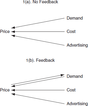
As a general rule, there are no basic direct statistical tests for determining the direction of causality; rather, the expert, when asked, should be prepared to defend his or her assumption based on an understanding of the underlying behavior evidence relating to the businesses or individuals involved.52
Although there is no single approach that is entirely suitable for estimating models when the dependent variable affects one or more explanatory variables, one possibility is for the expert to drop the questionable variable from the regression to determine whether the variable’s exclusion makes a difference. If it does not, the issue becomes moot. Another approach is for the expert to expand the multiple regression model by adding one or more equations that explain the relationship between the explanatory variable in question and the dependent variable.
Suppose, for example, that in a salary-based sex discrimination suit the defendant’s expert considers employer-evaluated test scores to be an appropriate explanatory variable for the dependent variable, salary. If the plaintiff were to provide information that the employer adjusted the test scores in a manner that penalized women, the assumption that salaries were determined by test scores and not that test scores were affected by salaries might be invalid. If it is clearly inappropriate,
52. There are statistical time-series tests for particular formulations of causality; see Pindyck & Rubinfeld, supra note 23, § 9.2.
the test-score variable should be removed from consideration. Alternatively, the information about the employer’s use of the test scores could be translated into a second equation in which a new dependent variable—test score—is related to workers’ salary and sex. A test of the hypothesis that salary and sex affect test scores would provide a suitable test of the absence of feedback.
2. To what extent are the explanatory variables correlated with each other?
It is essential in multiple regression analysis that the explanatory variable of interest not be correlated perfectly with one or more of the other explanatory variables. If there were perfect correlation between two variables, the expert could not separate out the effect of the variable of interest on the dependent variable from the effect of the other variable. In essence, there are two explanations for the same pattern in the data. Suppose, for example, that in a sex discrimination suit, a particular form of job experience is determined to be a valid source of high wages. If all men had the requisite job experience and all women did not, it would be impossible to tell whether wage differentials between men and women were the result of sex discrimination or differences in experience.
When two or more explanatory variables are correlated perfectly—that is, when there is perfect collinearity—one cannot estimate the regression parameters. The existing dataset does not allow one to distinguish between alternative competing explanations of the movement in the dependent variable. However, when two or more variables are highly, but not perfectly, correlated—that is, when there is multicollinearity—the regression can be estimated, but some concerns remain. The greater the multicollinearity between two variables, the less precise are the estimates of individual regression parameters, and an expert is less able to distinguish among competing explanations for the movement in the outcome variable (even though there is no problem in estimating the joint influence of the two variables and all other regression parameters).53
Fortunately, the reported regression statistics take into account any multicollinearity that might be present.54 It is important to note as a corollary, however, that a failure to find a strong relationship between a variable of interest and
53. See Griggs v. Duke Power Co., 401 U.S. 424 (1971) (The court argued that an education requirement was one rationalization of the data, but racial discrimination was another. If you had put both race and education in the regression, it would have been asking too much of the data to tell which variable was doing the real work, because education and race were so highly correlated in the market at that time.).
54. See Denny v. Westfield State College, 669 F. Supp. 1146, 1149 (D. Mass. 1987) (The court accepted the testimony of one expert that “the presence of multicollinearity would merely tend to overestimate the amount of error associated with the estimate…. In other words, p-values will be artificially higher than they would be if there were no multicollinearity present.”) (emphasis added); In re High Fructose Corn Syrup Antitrust Litig., 295 F.3d 651, 659 (7th Cir. Ill. 2002) (refusing to second-guess district court’s admission of regression analyses that addressed multicollinearity in different ways).
a dependent variable need not imply that there is no relationship.55 A relatively small sample, or even a large sample with substantial multicollinearity, may not provide sufficient information for the expert to determine whether there is a relationship.
3. To what extent are individual errors in the regression model independent?
If the expert calculated the parameters of a multiple regression model using as data the entire population, the estimates might still measure the model’s population parameters with error. Errors can arise for a number of reasons, including (1) the failure of the model to include the appropriate explanatory variables, (2) the failure of the model to reflect any nonlinearities that might be present, and (3) the inclusion of inappropriate variables in the model. (Of course, further sources of error will arise if a sample, or subset, of the population is used to estimate the regression parameters.)
It is useful to view the cumulative effect of all of these sources of modeling error as being represented by an additional variable, the error term, in the multiple regression model. An important assumption in multiple regression analysis is that the error term and each of the explanatory variables are independent of each other. (If the error term and an explanatory variable are independent, they are not correlated with each other.) To the extent this is true, the expert can estimate the parameters of the model without bias; the magnitude of the error term will affect the precision with which a model parameter is estimated, but will not cause that estimate to be consistently too high or too low.
The assumption of independence may be inappropriate in a number of circumstances. In some instances, failure of the assumption makes multiple regression analysis an unsuitable statistical technique; in other instances, modifications or adjustments within the regression framework can be made to accommodate the failure.
The independence assumption may fail, for example, in a study of individual behavior over time, in which an unusually high error value in one time period is likely to lead to an unusually high value in the next time period. For example, if an economic forecaster underpredicted this year’s Gross Domestic Product, he or she is likely to underpredict next year’s as well; the factor that caused the prediction error (e.g., an incorrect assumption about Federal Reserve policy) is likely to be a source of error in the future.
55. If an explanatory variable of concern and another explanatory variable are highly correlated, dropping the second variable from the regression can be instructive. If the coefficient on the explanatory variable of concern becomes significant, a relationship between the dependent variable and the explanatory variable of concern is suggested.
Alternatively, the assumption of independence may fail in a study of a group of firms at a particular point in time, in which error terms for large firms are systematically higher than error terms for small firms. For example, an analysis of the profitability of firms may not accurately account for the importance of advertising as a source of increased sales and profits. To the extent that large firms advertise more than small firms, the regression errors would be large for the large firms and small for the small firms. A third possibility is that the dependent variable varies at the individual level, but the explanatory variable of interest varies only at the level of a group. For example, an expert might be viewing the price of a product in an antitrust case as a function of a variable or variables that measure the marketing channel through which the product is sold (e.g., wholesale or retail). In this case, errors within each of the marketing groups are likely not to be independent. Failure to account for this could cause the expert to overstate the statistical significance of the regression parameters.
In some instances, there are statistical tests that are appropriate for evaluating the independence assumption.56 If the assumption has failed, the expert should ask first whether the source of the lack of independence is the omission of an important explanatory variable from the regression. If so, that variable should be included when possible, or the potential effect of its omission should be estimated when inclusion is not possible. If there is no important missing explanatory variable, the expert should apply one or more procedures that modify the standard multiple regression technique to allow for more accurate estimates of the regression parameters.57
4. To what extent are the regression results sensitive to individual data points?
Estimated regression coefficients can be highly sensitive to particular data points. Suppose, for example, that one data point deviates greatly from its expected value, as indicated by the regression equation, while the remaining data points show
56. In a time-series analysis, the correlation of error values over time, the “serial correlation,” can be tested (in most instances) using a number of tests, including the Durbin-Watson test. The possibility that some error terms are consistently high in magnitude and others are systematically low, heteroscedasticity can also be tested in a number of ways. See, e.g., Pindyck & Rubinfeld, supra note 23, at 146–59. When serial correlation and/or heteroscedasticity are present, the standard errors associated with the estimated coefficients must be modified. For a discussion of the use of such “robust” standard errors, see Jeffrey M. Wooldridge, Introductory Econometrics: A Modern Approach, ch. 8 (4th ed. 2009).
57. When serial correlation is present, a number of closely related statistical methods are appropriate, including generalized differencing (a type of generalized least squares) and maximum likelihood estimation. When heteroscedasticity is the problem, weighted least squares and maximum likelihood estimation are appropriate. See, e.g., id. All these techniques are readily available in a number of statistical computer packages. They also allow one to perform the appropriate statistical tests of the significance of the regression coefficients.
little deviation. It would not be unusual in this situation for the coefficients in a multiple regression to change substantially if the data point in question were removed from the sample.
Evaluating the robustness of multiple regression results is a complex endeavor. Consequently, there is no agreed set of tests for robustness that analysts should apply. In general, it is important to explore the reasons for unusual data points. If the source is an error in recording data, the appropriate corrections can be made. If all the unusual data points have certain characteristics in common (e.g., they all are associated with a supervisor who consistently gives high ratings in an equal pay case), the regression model should be modified appropriately.
One generally useful diagnostic technique is to determine to what extent the estimated parameter changes as each data point in the regression analysis is dropped from the sample. An influential data point—a point that causes the estimated parameter to change substantially—should be studied further to determine whether mistakes were made in the use of the data or whether important explanatory variables were omitted.58
5. To what extent are the data subject to measurement error?
In multiple regression analysis it is assumed that variables are measured accurately.59 If there are measurement errors in the dependent variable, estimates of regression parameters will be less accurate, although they will not necessarily be biased. However, if one or more independent variables are measured with error, the corresponding parameter estimates are likely to be biased, typically toward zero (and other coefficient estimates are likely to be biased as well).
To understand why, suppose that the dependent variable, salary, is measured without error, and the explanatory variable, experience, is subject to measurement error. (Seniority or years of experience should be accurate, but the type of experience is subject to error, because applicants may overstate previous job responsibilities.) As the measurement error increases, the estimated parameter associated with the experience variable will tend toward zero, that is, eventually, there will be no relationship between salary and experience.
It is important for any source of measurement error to be carefully evaluated. In some circumstances, little can be done to correct the measurement-error prob-
58. A more complete and formal treatment of the robustness issue appears in David A. Belsley et al., Regression Diagnostics: Identifying Influential Data and Sources of Collinearity 229–44 (1980). For a useful discussion of the detection of outliers and the evaluation of influential data points, see R.D. Cook & S. Weisberg, Residuals and Influence in Regression (Monographs on Statistics and Applied Probability No. 18, 1982). For a broad discussion of robust regression methods, see Peer J. Rouseeuw & Annick M. Leroy, Robust Regression and Outlier Detection (2004).
59. Inaccuracy can occur not only in the precision with which a particular variable is measured, but also in the precision with which the variable to be measured corresponds to the appropriate theoretical construct specified by the regression model.
lem; the regression results must be interpreted in that light. In other circumstances, however, the expert can correct measurement error by finding a new, more reliable data source. Finally, alternative estimation techniques (using related variables that are measured without error) can be applied to remedy the measurement-error problem in some situations.60
Multiple regression analysis is taught to students in extremely diverse fields, including statistics, economics, political science, sociology, psychology, anthropology, public health, and history. Nonetheless, the methodology is difficult to master, necessitating a combination of technical skills (the science) and experience (the art). This naturally raises two questions:
- Who should be qualified as an expert?
- When and how should the court appoint an expert to assist in the evaluation of statistical issues, including those relating to multiple regression?
A. Who Should Be Qualified as an Expert?
Any individual with substantial training in and experience with multiple regression and other statistical methods may be qualified as an expert.61 A doctoral degree in a discipline that teaches theoretical or applied statistics, such as economics, history, and psychology, usually signifies to other scientists that the proposed expert meets this preliminary test of the qualification process.
The decision to qualify an expert in regression analysis rests with the court. Clearly, the proposed expert should be able to demonstrate an understanding of the discipline. Publications relating to regression analysis in peer-reviewed journals, active memberships in related professional organizations, courses taught on regression methods, and practical experience with regression analysis can indicate a professional’s expertise. However, the expert’s background and experience with the specific issues and tools that are applicable to a particular case should also be considered during the qualification process. Thus, if the regression methods are being utilized to evaluate damages in an antitrust case, the qualified expert should have sufficient qualifications in economic analysis as well as statistics. An individual whose expertise lies solely with statistics will be limited in his or her ability to evaluate the usefulness of alternative economic models. Similarly, if a case involves
60. See, e.g., Pindyck & Rubinfeld, supra note 23, at 178–98 (discussion of instrumental variables estimation).
61. A proposed expert whose only statistical tool is regression analysis may not be able to judge when a statistical analysis should be based on an approach other than regression analysis.
eyewitness identification, a background in psychology as well as statistics may provide essential qualifying elements.
B. Should the Court Appoint a Neutral Expert?
There are conflicting views on the issue of whether court-appointed experts should be used. In complex cases in which two experts are presenting conflicting statistical evidence, the use of a “neutral” court-appointed expert can be advantageous. There are those who believe, however, that there is no such thing as a truly “neutral” expert. In any event, if an expert is chosen, that individual should have substantial expertise and experience—ideally, someone who is respected by both plaintiffs and defendants.62
The appointment of such an expert is likely to influence the presentation of the statistical evidence by the experts for the parties in the litigation. The neutral expert will have an incentive to present a balanced position that relies on broad principles for which there is consensus in the community of experts. As a result, the parties’ experts can be expected to present testimony that confronts core issues that are likely to be of concern to the court and that is sufficiently balanced to be persuasive to the court-appointed expert.63
Rule 706 of the Federal Rules of Evidence governs the selection and instruction of court-appointed experts. In particular:
- The expert should be notified of his or her duties through a written court order or at a conference with the parties.
- The expert should inform the parties of his or her findings orally or in writing.
- If deemed appropriate by the court, the expert should be available to testify and may be deposed or cross-examined by any party.
- The court must determine the expert’s compensation.64
- The parties should be free to utilize their own experts.
Although not required by Rule 706, it will usually be advantageous for the court to opt for the appointment of a neutral expert as early in the litigation process as possible. It will also be advantageous to minimize any ex parte contact with
62. Judge Posner notes in In re High Fructose Corn Syrup Antitrust Litig., 295 F.2d 651, 665 (7th Cir., 2002), “the judge and jury can repose a degree of confidence in his testimony that it could not repose in that of a party’s witness. The judge and the jury may not understand the neutral expert perfectly but at least they will know that he has no axe to grind, and so, to a degree anyway, they will be able to take his testimony on faith.”
63. For a discussion of the presentation of expert evidence generally, including the use of court-appointed experts, see Samuel R. Gross, Expert Evidence, 1991 Wis. L. Rev. 1113 (1991).
64. Although Rule 706 states that the compensation must come from public funds, complex litigation may be sufficiently costly as to require that the parties share the costs of the neutral expert.
the neutral expert; this will diminish the possibility that one or both parties will come to the view that the court’s ultimate opinion was unreasonably influenced by the neutral expert.
Rule 706 does not offer specifics as to the process of appointment of a court-appointed expert. One possibility is to have the parties offer a short list of possible appointees. If there was no common choice, the court could select from the combined list, perhaps after allowing each party to exercise one or more peremptory challenges. Another possibility is to obtain a list of recommended experts from a selection of individuals known to be experts in the field.
V. Presentation of Statistical Evidence
The costs of evaluating statistical evidence can be reduced and the precision of that evidence increased if the discovery process is used effectively. In evaluating the admissibility of statistical evidence, courts should consider the following issues:
- Has the expert provided sufficient information to replicate the multiple regression analysis?
- Are the expert’s methodological choices reasonable, or are they arbitrary and unjustified?
A. What Disagreements Exist Regarding Data on Which the Analysis Is Based?
In general, a clear and comprehensive statement of the underlying research methodology is a requisite part of the discovery process. The expert should be encouraged to reveal both the nature of the experimentation carried out and the sensitivity of the results to the data and to the methodology.
The following suggestions are useful requirements that can substantially improve the discovery process:
- To the extent possible, the parties should be encouraged to agree to use a common database. Even if disagreement about the significance of the data remains, early agreement on a common database can help focus the discovery process on the important issues in the case.
- A party that offers data to be used in statistical work, including multiple regression analysis, should be encouraged to provide the following to the other parties: (a) a hard copy of the data when available and manageable in size, along with the underlying sources; (b) computer disks or tapes on which the data are recorded; (c) complete documentation of the disks or tapes; (d) computer programs that were used to generate the data (in hard
-
copy if necessary, but preferably on a computer disk or tape, or both); and (e) documentation of such computer programs. The documentation should be sufficiently complete and clear so that the opposing expert can reproduce all of the statistical work.
- A party offering data should make available the personnel involved in the compilation of such data to answer the other parties’ technical questions concerning the data and the methods of collection or compilation.
- A party proposing to offer an expert’s regression analysis at trial should ask the expert to fully disclose (a) the database and its sources,65 (b) the method of collecting the data, and (c) the methods of analysis. When possible, this disclosure should be made sufficiently in advance of trial so that the opposing party can consult its experts and prepare cross-examination. The court must decide on a case-by-case basis where to draw the disclosure line.
- An opposing party should be given the opportunity to object to a database or to a proposed method of analysis of the database to be offered at trial. Objections may be to simple clerical errors or to more complex issues relating to the selection of data, the construction of variables, and, on occasion, the particular form of statistical analysis to be used. Whenever possible, these objections should be resolved before trial.
- The parties should be encouraged to resolve differences as to the appropriateness and precision of the data to the extent possible by informal conference. The court should make an effort to resolve differences before trial.
These suggestions are motivated by the objective of improving the discovery process to make it more informative. The fact that these questions may raise some doubts or concerns about a particular regression model should not be taken to mean that the model does not provide useful information. It does, however, take considerable skill for an expert to determine the extent to which information is useful when the model being utilized has some shortcomings.
B. Which Database Information and Analytical Procedures Will Aid in Resolving Disputes over Statistical Studies?66
To help resolve disputes over statistical studies, experts should follow the guidelines below when presenting database information and analytical procedures:
65. These sources would include all variables used in the statistical analyses conducted by the expert, not simply those variables used in a final analysis on which the expert expects to rely.
66. For a more complete discussion of these requirements, see The Evolving Role of Statistical Assessments as Evidence in the Courts, app. F at 256 (Stephen E. Fienberg ed., 1989) (Recommended
- The expert should state clearly the objectives of the study, as well as the time frame to which it applies and the statistical population to which the results are being projected.
- The expert should report the units of observation (e.g., consumers, businesses, or employees).
- The expert should clearly define each variable.
- The expert should clearly identify the sample for which data are being studied,67 as well as the method by which the sample was obtained.
- The expert should reveal if there are missing data, whether caused by a lack of availability (e.g., in business data) or nonresponse (e.g., in survey data), and the method used to handle the missing data (e.g., deletion of observations).
- The expert should report investigations into errors associated with the choice of variables and assumptions underlying the regression model.
- If samples were chosen randomly from a population (i.e., probability sampling procedures were used),68 the expert should make a good-faith effort to provide an estimate of a sampling error, the measure of the difference between the sample estimate of a parameter (such as the mean of a dependent variable under study), and the (unknown) population parameter (the population mean of the variable).69
- If probability sampling procedures were not used, the expert should report the set of procedures that was used to minimize sampling errors.
Standards on Disclosure of Procedures Used for Statistical Studies to Collect Data Submitted in Evidence in Legal Cases).
67. The sample information is important because it allows the expert to make inferences about the underlying population.
68. In probability sampling, each representative of the population has a known probability of being in the sample. Probability sampling is ideal because it is highly structured, and in principle, it can be replicated by others. Nonprobability sampling is less desirable because it is often subjective, relying to a large extent on the judgment of the expert.
69. Sampling error is often reported in terms of standard errors or confidence intervals. See Appendix, infra, for details.
Appendix: The Basics of Multiple Regression
This appendix illustrates, through examples, the basics of multiple regression analysis in legal proceedings. Often, visual displays are used to describe the relationship between variables that are used in multiple regression analysis. Figure 2 is a scatterplot that relates scores on a job aptitude test (shown on the x-axis) and job performance ratings (shown on the y-axis). Each point on the scatterplot shows where a particular individual scored on the job aptitude test and how his or her job performance was rated. For example, the individual represented by Point A in Figure 2 scored 49 on the job aptitude test and had a job performance rating of 62.
Figure 2. Scatterplot of scores on a job aptitude test relative to job performance rating.
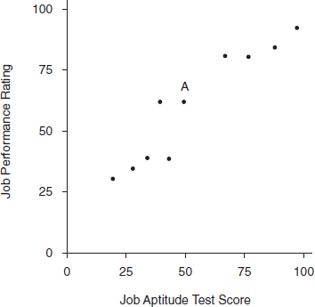
The relationship between two variables can be summarized by a correlation coefficient, which ranges in value from −1 (a perfect negative relationship) to +1 (a perfect positive relationship). Figure 3 depicts three possible relationships between the job aptitude variable and the job performance variable. In Figure 3(a), there is a positive correlation: In general, higher job performance ratings are associated with higher aptitude test scores, and lower job performance ratings are associated with lower aptitude test scores. In Figure 3(b), the correlation is
negative: Higher job performance ratings are associated with lower aptitude test scores, and lower job performance ratings are associated with higher aptitude test scores. Positive and negative correlations can be relatively strong or relatively weak. If the relationship is sufficiently weak, there is effectively no correlation, as is illustrated in Figure 3(c).
Figure 3. Correlation between the job aptitude variable and the job performance variable: (a) positive correlation, (b) negative correlation, (c) weak relationship with no correlation.
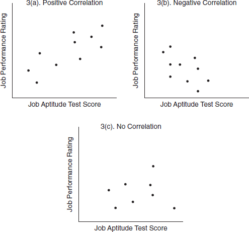
Multiple regression analysis goes beyond the calculation of correlations; it is a method in which a regression line is used to relate the average of one variable—the dependent variable—to the values of other explanatory variables. As a result, regression analysis can be used to predict the values of one variable using the values of others. For example, if average job performance ratings depend on aptitude test scores, regression analysis can use information about test scores to predict job performance.
A regression line is the best-fitting straight line through a set of points in a scatterplot. If there is only one explanatory variable, the straight line is defined by the equation
| Y = a + bX. | (1) |
In equation (1), a is the intercept of the line with the y-axis when X equals 0, and b is the slope—the change in the dependent variable associated with a 1-unit change in the explanatory variable. In Figure 4, for example, when the aptitude test score is 0, the predicted (average) value of the job performance rating is the intercept, 18.4. Also, for each additional point on the test score, the job performance rating increases .73 units, which is given by the slope .73. Thus, the estimated regression line is
| Y = 18.4 + .73X. | (2) |
The regression line typically is estimated using the standard method of least squares, where the values of a and b are calculated so that the sum of the squared deviations of the points from the line are minimized. In this way, positive deviations and negative deviations of equal size are counted equally, and large deviations are counted more than small deviations. In Figure 4 the deviation lines are verti-
Figure 4. Regression line.
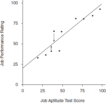
cal because the equation is predicting job performance ratings from aptitude test scores, not aptitude test scores from job performance ratings.
The important variables that systematically might influence the dependent variable, and for which data can be obtained, typically should be included explicitly in a statistical model. All remaining influences, which should be small individually, but can be substantial in the aggregate, are included in an additional random error term.70 Multiple regression is a procedure that separates the systematic effects (associated with the explanatory variables) from the random effects (associated with the error term) and also offers a method of assessing the success of the process.
When there are an arbitrary number of explanatory variables, the linear regression model takes the following form:
| Y = β0 + β1X1 + β2X2 +…+ βkXk + ε | (3) |
where Y represents the dependent variable, such as the salary of an employee, and X1…Xk represent the explanatory variables (e.g., the experience of each employee and his or her sex, coded as a 1 or 0, respectively). The error term, e, represents the collective unobservable influence of any omitted variables. In a linear regression, each of the terms being added involves unknown parameters, β0, β1,…βk,71 which are estimated by “fitting” the equation to the data using least squares.
Each estimated coefficient βk measures how the dependent variable Y responds, on average, to a change in the corresponding covariate Xk, after “controlling for” all the other covariates. The informal phrase “controlling for” has a specific statistical meaning. Consider the following three-step procedure. First, we calculate the residuals from a regression of Y on all covariates other than Xk. Second, we calculate the residuals of a regression of Xk on all the other covariates. Third, and finally, we regress the first residual variable on the second residual variable. The resulting coefficient will be identically equal to βk. Thus, the coeffi-
70. It is clearly advantageous for the random component of the regression relationship to be small relative to the variation in the dependent variable.
71. The variables themselves can appear in many different forms. For example, Y might represent the logarithm of an employee’s salary, and X1 might represent the logarithm of the employee’s years of experience. The logarithmic representation is appropriate when Y increases exponentially as X increases—for each unit increase in X, the corresponding increase in Y becomes larger and larger. For example, if an expert were to graph the growth of the U.S. population (Y) over time (t), the following equation might be appropriate:
log(Y) = β0 + β1log(t).
cient in a multiple regression represents the slope of the line “Y, adjusted for all covariates other than Xk versus Xk adjusted for all the other covariates.”72
Most statisticians use the least squares regression technique because of its simplicity and its desirable statistical properties. As a result, it also is used frequently in legal proceedings.
1. Specifying the regression model
Suppose an expert wants to analyze the salaries of women and men at a large publishing house to discover whether a difference in salaries between employees with similar years of work experience provides evidence of discrimination.73 To begin with the simplest case, Y, the salary in dollars per year, represents the dependent variable to be explained, and X1 represents the explanatory variable—the number of years of experience of the employee. The regression model would be written
| Y = β0 + β1X1 + ε. | (4) |
In equation (4), β0 and β1 are the parameters to be estimated from the data, and e is the random error term. The parameter β0 is the average salary of all employees with no experience. The parameter β1 measures the average effect of an additional year of experience on the average salary of employees.
Once the parameters in a regression equation, such as equation (3), have been estimated, the fitted values for the dependent variable can be calculated. If we denote the estimated regression parameters, or regression coefficients, for the model in equation (3) by β0, β1,…βk, the fitted values for Y, denoted Ŷ, are given by
| Ŷ = β0 + β1X1 + β2X2 +…βkXk. | (5) |
Figure 5 illustrates this for the example involving a single explanatory variable. The data are shown as a scatter of points; salary is on the vertical axis, and years of experience is on the horizontal axis. The estimated regression line is drawn through the data points. It is given by
| Ŷ = $15,000 + $2000X1. | (6) |
72. In econometrics, this is known as the Frisch–Waugh–Lovell theorem.
73. The regression results used in this example are based on data for 1715 men and women, which were used by the defense in a sex discrimination case against the New York Times that was settled in 1978. Professor Orley Ashenfelter, Department of Economics, Princeton University, provided the data.
Figure 5. Goodness of fit.
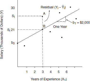
Thus, the fitted value for the salary associated with an individual’s years of experience X1i is given by
| Ŷi= β0 + β1X1i (at Point B). | (7) |
The intercept of the straight line is the average value of the dependent variable when the explanatory variable or variables are equal to 0; the intercept β0 is shown on the vertical axis in Figure 5. Similarly, the slope of the line measures the (average) change in the dependent variable associated with a unit increase in an explanatory variable; the slope β1 also is shown. In equation (6), the intercept $15,000 indicates that employees with no experience earn $15,000 per year. The slope parameter implies that each year of experience adds $2000 to an “average” employee’s salary.
Now, suppose that the salary variable is related simply to the sex of the employee. The relevant indicator variable, often called a dummy variable, is X2, which is equal to 1 if the employee is male, and 0 if the employee is female. Suppose the regression of salary Y on X2 yields the following result: Y = $30,449 + $10,979X2. The coefficient $10,979 measures the difference between the average salary of men and the average salary of women.74
74. To understand why, note that when X2 equals 0, the average salary for women is $30,449 + $10,979*0 = $30,449. Correspondingly, when X2 = 1, the average salary for men is $30,449 + $10,979*1 = $41,428. The difference, $41,428 − $30,449, is $10,979.
a. Regression residuals
For each data point, the regression residual is the difference between the actual values and fitted values of the dependent variable. Suppose, for example, that we are studying an individual with 3 years of experience and a salary of $27,000. According to the regression line in Figure 5, the average salary of an individual with 3 years of experience is $21,000. Because the individual’s salary is $6000 higher than the average salary, the residual (the individual’s salary minus the average salary) is $6000. In general, the residual e associated with a data point, such as Point A in Figure 5, is given by ei = Yi − Ŷi. Each data point in the figure has a residual, which is the error made by the least squares regression method for that individual.
b. Nonlinearities
Nonlinear models account for the possibility that the effect of an explanatory variable on the dependent variable may vary in magnitude as the level of the explanatory variable changes. One useful nonlinear model uses interactions among variables to produce this effect. For example, suppose that
| S = β1 +β2SEX + β3EXP + β4(EXP)(SEX) + ε | (8) |
where S is annual salary, SEX is equal to 1 for women and 0 for men, EXP represents years of job experience, and e is a random error term. The coefficient β2 measures the difference in average salary (across all experience levels) between men and women for employees with no experience. The coefficient β3 measures the effect of experience on salary for men (when SEX = 0), and the coefficient β4 measures the difference in the effect of experience on salary between men and women. It follows, for example, that the effect of 1 year of experience on salary for men is β3, whereas the comparable effect for women is β3 + β4.75
C. Interpreting Regression Results
To explain how regression results are interpreted, we can expand the earlier example associated with Figure 5 to consider the possibility of an additional explanatory variable—the square of the number of years of experience, X3. The X3 variable is designed to capture the fact that for most individuals, salaries increase with experience, but eventually salaries tend to level off. The estimated regression line using the third additional explanatory variable, as well as the first explanatory variable for years of experience (X1) and the dummy variable for sex (X2), is
75. Estimating a regression in which there are interaction terms for all explanatory variables, as in equation (8), is essentially the same as estimating two separate regressions, one for men and one for women.
| Ŷ = $14,085 + $2323X1 + $1675X2 − $36X3. | (9) |
The importance of including relevant explanatory variables in a regression model is illustrated by the change in the regression results after the X3 and X1 variables are added. The coefficient on the variable X2 measures the difference in the salaries of men and women while controlling for the effect of experience. The differential of $1675 is substantially lower than the previously measured differential of $10,979. Clearly, failure to control for job experience in this example leads to an overstatement of the difference in salaries between men and women.
Now consider the interpretation of the explanatory variables for experience, X1 and X3. The positive sign on the X1 coefficient shows that salary increases with experience. The negative sign on the X3 coefficient indicates that the rate of salary increase decreases with experience. To determine the combined effect of the variables X1 and X3, some simple calculations can be made. For example, consider how the average salary of women (X2 = 0) changes with the level of experience. As experience increases from 0 to 1 year, the average salary increases by $2251, from $14,085 to $16,336. However, women with 2 years of experience earn only $2179 more than women with 1 year of experience, and women with 1 year of experience earn only $2127 more than women with 2 years. Furthermore, women with 7 years of experience earn $28,582 per year, which is only $1855 more than the $26,727 earned by women with 6 years of experience.76Figure 6 illustrates the results: The regression line shown is for women’s salaries; the corresponding line for men’s salaries would be parallel and $1675 higher.
D. Determining the Precision of the Regression Results
Least squares regression provides not only parameter estimates that indicate the direction and magnitude of the effect of a change in the explanatory variable on the dependent variable, but also an estimate of the reliability of the parameter estimates and a measure of the overall goodness of fit of the regression model. Each of these factors is considered in turn.
1. Standard errors of the coefficients and t-statistics
Estimates of the true but unknown parameters of a regression model are numbers that depend on the particular sample of observations under study. If a different sample were used, a different estimate would be calculated.77 If the expert continued to collect more and more samples and generated additional estimates, as might happen when new data became available over time, the estimates of each
76. These numbers can be calculated by substituting different values of X1 and X3 in equation (9).
77. The least squares formula that generates the estimates is called the least squares estimator, and its values vary from sample to sample.
Figure 6. Regression slope for women’s salaries and men’s salaries.
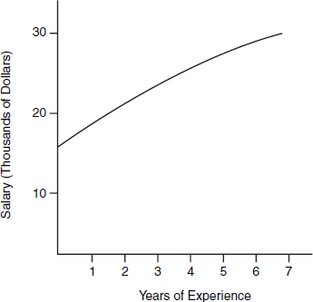
parameter would follow a probability distribution (i.e., the expert could determine the percentage or frequency of the time that each estimate occurs). This probability distribution can be summarized by a mean and a measure of dispersion around the mean, a standard deviation, which usually is referred to as the standard error of the coefficient, or the standard error (SE).78
Suppose, for example, that an expert is interested in estimating the average price paid for a gallon of unleaded gasoline by consumers in a particular geographic area of the United States at a particular point in time. The mean price for a sample of 10 gas stations might be $1.25, while the mean for another sample might be $1.29, and the mean for a third, $1.21. On this basis, the expert also could calculate the overall mean price of gasoline to be $1.25 and the standard deviation to be $0.04.
Least squares regression generalizes this result, by calculating means whose values depend on one or more explanatory variables. The standard error of a regression coefficient tells the expert how much parameter estimates are likely to vary from sample to sample. The greater the variation in parameter estimates from sample to sample, the larger the standard error and consequently the less reliable the regression results. Small standard errors imply results that are likely to
78. See David H. Kaye & David A. Freedman, Reference Guide on Statistics, Section IV.A, in this manual.
be similar from sample to sample, whereas results with large standard errors show more variability.
Under appropriate assumptions, the least squares estimators provide “best” determinations of the true underlying parameters.79 In fact, least squares has several desirable properties. First, least squares estimators are unbiased. Intuitively, this means that if the regression were calculated repeatedly with different samples, the average of the many estimates obtained for each coefficient would be the true parameter. Second, least squares estimators are consistent; if the sample were very large, the estimates obtained would come close to the true parameters. Third, least squares is efficient, in that its estimators have the smallest variance among all (linear) unbiased estimators.
If the further assumption is made that the probability distribution of each of the error terms is known, statistical statements can be made about the precision of the coefficient estimates. For relatively large samples (often, thirty or more data points will be sufficient for regressions with a small number of explanatory variables), the probability that the estimate of a parameter lies within an interval of 2 standard errors around the true parameter is approximately .95, or 95%. A frequent, although not always appropriate, assumption in statistical work is that the error term follows a normal distribution, from which it follows that the estimated parameters are normally distributed. The normal distribution has the property that the area within 1.96 standard errors of the mean is equal to 95% of the total area. Note that the normality assumption is not necessary for least squares to be used, because most of the properties of least squares apply regardless of normality.
In general, for any parameter estimate b, the expert can construct an interval around b such that there is a 95% probability that the interval covers the true parameter. This 95% confidence interval80 is given by81
| b ± 1.96 (SE of b). | (10) |
The expert can test the hypothesis that a parameter is actually equal to 0 (often stated as testing the null hypothesis) by looking at its t-statistic, which is defined as
| (11) |
79. The necessary assumptions of the regression model include (a) the model is specified correctly, (b) errors associated with each observation are drawn randomly from the same probability distribution and are independent of each other, (c) errors associated with each observation are independent of the corresponding observations for each of the explanatory variables in the model, and (d) no explanatory variable is correlated perfectly with a combination of other variables.
80. Confidence intervals are used commonly in statistical analyses because the expert can never be certain that a parameter estimate is equal to the true population parameter.
81. If the number of data points in the sample is small, the standard error must be multiplied by a number larger than 1.96.
If the t-statistic is less than 1.96 in magnitude, the 95% confidence interval around b must include 0.82 Because this means that the expert cannot reject the hypothesis that β equals 0, the estimate, whatever it may be, is said to be not statistically significant. Conversely, if the t-statistic is greater than 1.96 in absolute value, the expert concludes that the true value of β is unlikely to be 0 (intuitively, b is “too far” from 0 to be consistent with the true value of β being 0). In this case, the expert rejects the hypothesis that β equals 0 and calls the estimate statistically significant. If the null hypothesis β equals 0 is true, using a 95% confidence level will cause the expert to falsely reject the null hypothesis 5% of the time. Consequently, results often are said to be significant at the 5% level.83
As an example, consider a more complete set of regression results associated with the salary regression described in equation (9):
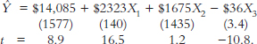 |
(12) |
The standard error of each estimated parameter is given in parentheses directly below the parameter, and the corresponding t-statistics appear below the standard error values.
Consider the coefficient on the dummy variable X2. It indicates that $1675 is the best estimate of the mean salary difference between men and women. However, the standard error of $1435 is large in relation to its coefficient $1675. Because the standard error is relatively large, the range of possible values for measuring the true salary difference, the true parameter, is great. In fact, a 95% confidence interval is given by
| $1675 ± $1435 ∙ 1.96 = $1675 ± $2813. | (13) |
In other words, the expert can have 95% confidence that the true value of the coefficient lies between −$1138 and $4488. Because this range includes 0, the effect of sex on salary is said to be insignificantly different from 0 at the 5% level. The t value of 1.2 is equal to $1675 divided by $1435. Because this t-statistic is less than 1.96 in magnitude (a condition equivalent to the inclusion of a 0 in the above confidence interval), the sex variable again is said to be an insignificant determinant of salary at the 5% level of significance.
82. The t-statistic applies to any sample size. As the sample gets large, the underlying distribution, which is the source of the t-statistic (Student’s t-distribution), approximates the normal distribution.
83. A t-statistic of 2.57 in magnitude or greater is associated with a 99% confidence level, or a 1% level of significance, that includes a band of 2.57 standard deviations on either side of the estimated coefficient.
Note also that experience is a highly significant determinant of salary, because both the X1 and the X3 variables have t-statistics substantially greater than 1.96 in magnitude. More experience has a significant positive effect on salary, but the size of this effect diminishes significantly with experience.
Reported regression results usually contain not only the point estimates of the parameters and their standard errors or t-statistics, but also other information that tells how closely the regression line fits the data. One statistic, the standard error of the regression (SER), is an estimate of the overall size of the regression residuals.84 An SER of 0 would occur only when all data points lie exactly on the regression line—an extremely unlikely possibility. Other things being equal, the larger the SER, the poorer the fit of the data to the model.
For a normally distributed error term, the expert would expect approximately 95% of the data points to lie within 2 SERs of the estimated regression line, as shown in Figure 7 (in Figure 7, the SER is approximately $5000).
Figure 7. Standard error of the regression.
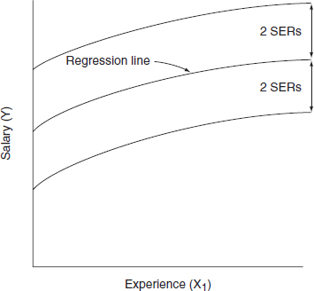
84. More specifically, it is a measure of the standard deviation of the regression error e. It sometimes is called the root mean squared error of the regression line.
R-squared (R2) is a statistic that measures the percentage of variation in the dependent variable that is accounted for by all the explanatory variables.85 Thus, R2 provides a measure of the overall goodness of fit of the multiple regression equation. Its value ranges from 0 to 1. An R2 of 0 means that the explanatory variables explain none of the variation of the dependent variable; an R2 of 1 means that the explanatory variables explain all of the variation. The R2 associated with equation (12) is .56. This implies that the three explanatory variables explain 56% of the variation in salaries.
What level of R2, if any, should lead to a conclusion that the model is satisfactory? Unfortunately, there is no clear-cut answer to this question, because the magnitude of R2 depends on the characteristics of the data being studied and, in particular, whether the data vary over time or over individuals. Typically, an R2 is low in cross-sectional studies in which differences in individual behavior are explained. It is likely that these individual differences are caused by many factors that cannot be measured. As a result, the expert cannot hope to explain most of the variation. In time-series studies, in contrast, the expert is explaining the movement of aggregates over time. Because most aggregate time series have substantial growth, or trend, in common, it will not be difficult to “explain” one time series using another time series, simply because both are moving together. It follows as a corollary that a high R2 does not by itself mean that the variables included in the model are the appropriate ones.
As a general rule, courts should be reluctant to rely solely on a statistic such as R2 to choose one model over another. Alternative procedures and tests are available.86
3. Sensitivity of least squares regression results
The least squares regression line can be sensitive to extreme data points. This sensitivity can be seen most easily in Figure 8. Assume initially that there are only three data points, A, B, and C, relating information about X1 to the variable Y. The least squares line describing the best-fitting relationship between Points A, B, and C is represented by Line 1. Point D is called an outlier because it lies far from the regression line that fits the remaining points. When a new, best-fitting least squares line is reestimated to include Point D, Line 2 is obtained. Figure 8 shows that the outlier Point D is an influential data point, because it has a dominant effect on the slope and intercept of the least squares line. Because least squares attempts to minimize the sum of squared deviations, the sensitivity of the line to individual points sometimes can be substantial.87
85. The variation is the square of the difference between each Y value and the average Y value, summed over all the Y values.
86. These include F-tests and specification error tests. See Pindyck & Rubinfeld, supra note 23, at 88–95, 128–36, 194–98.
87. This sensitivity is not always undesirable. In some instances it may be much more important to predict Point D when a big change occurs than to measure the effects of small changes accurately.
Figure 8. Least squares regression.
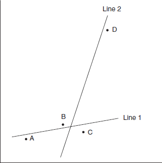
What makes the influential data problem even more difficult is that the effect of an outlier may not be seen readily if deviations are measured from the final regression line. The reason is that the influence of Point D on Line 2 is so substantial that its deviation from the regression line is not necessarily larger than the deviation of any of the remaining points from the regression line.88 Although they are not as popular as least squares, alternative estimation techniques that are less sensitive to outliers, such as robust estimation, are available.
E. Reading Multiple Regression Computer Output
Statistical computer packages that report multiple regression analyses vary to some extent in the information they provide and the form that the information takes. Table 1 contains a sample of the basic computer output that is associated with equation (9).
88. The importance of an outlier also depends on its location in the dataset. Outliers associated with relatively extreme values of explanatory variables are likely to be especially influential. See, e.g., Fisher v. Vassar College, 70 F.3d 1420, 1436 (2d Cir. 1995) (court required to include assessment of “service in academic community,” because concept was too amorphous and not a significant factor in tenure review), rev’d on other grounds, 114 F.3d 1332 (2d Cir. 1997) (en banc).
Table 1. Regression Output
| Dependent variable: Y | SSE DFE MSE | 62346266124 561 111134164 | F-test Prob > F R2 | 174.71 0.0001 0.556 | |
| Variable DF | Parameter Estimate | Standard Error | t-Statistic | Prob >|t| | |
| Intercept 1 | 14,084.89 | 1577.484 | 8.9287 | .0001 | |
| X1 1 | 2323.17 | 140.70 | 16.5115 | .0001 | |
| X2 1 | 1675.11 | 1435.422 | 1.1670 | .2437 | |
| X3 1 | −36.71 | 3.41 | −10.7573 | .0001 | |
Note: SSE = sum of squared errors; DFE = degrees of freedom associated with the error term; MSE = mean squared error; DF = degrees of freedom; Prob = probability.
In the lower portion of Table 1, note that the parameter estimates, the standard errors, and the t-statistics match the values given in equation (12).89 The variable “Intercept” refers to the constant term b0 in the regression. The column “DF” represents degrees of freedom. The “1” signifies that when the computer calculates the parameter estimates, each variable that is added to the linear regression adds an additional constraint that must be satisfied. The column labeled “Prob > |t|” lists the two-tailed p-values associated with each estimated parameter; the p-value measures the observed significance level—the probability of getting a test statistic as extreme or more extreme than the observed number if the model parameter is in fact 0. The very low p-values on the variables X1 and X3 imply that each variable is statistically significant at less than the 1% level—both highly significant results. In contrast, the X2 coefficient is only significant at the 24% level, implying that it is insignificant at the traditional 5% level. Thus, the expert cannot reject with confidence the null hypothesis that salaries do not differ by sex after the expert has accounted for the effect of experience.
The top portion of Table 1 provides data that relate to the goodness of fit of the regression equation. The sum of squared errors (SSE) measures the sum of the squares of the regression residuals—the sum that is minimized by the least squares procedure. The degrees of freedom associated with the error term (DFE) are given by the number of observations minus the number of parameters that were estimated. The mean squared error (MSE) measures the variance of the error term (the square of the standard error of the regression). MSE is equal to SSE divided by DFE.
89. Computer programs give results to more decimal places than are meaningful. This added detail should not be seen as evidence that the regression results are exact.
The R2 of 0.556 indicates that 55.6% of the variation in salaries is explained by the regression variables, X1, X2, and X3. Finally, the F-test is a test of the null hypothesis that all regression coefficients (except the intercept) are jointly equal to 0—that there is no linear association between the dependent variable and any of the explanatory variables. This is equivalent to the null hypothesis that R2 is equal to 0. In this case, the F-ratio of 174.71 is sufficiently high that the expert can reject the null hypothesis with a very high degree of confidence (i.e., with a 1% level of significance).
In general, a forecast is a prediction made about the values of the dependent variable using information about the explanatory variables. Often, ex ante forecasts are performed; in this situation, values of the dependent variable are predicted beyond the sample (e.g., beyond the time period in which the model has been estimated). However, ex post forecasts are frequently used in damage analyses.90 An ex post forecast has a forecast period such that all values of the dependent and explanatory variables are known; ex post forecasts can be checked against existing data and provide a direct means of evaluation.
For example, to calculate the forecast for the salary regression discussed above, the expert uses the estimated salary equation
| Ŷ = $14,085 + $2323X1 + $1675X2 − $36X3. | (14) |
To predict the salary of a man with 2 years’ experience, the expert calculates
| Ŷ (2) = $14,085 + ($2323 ∙ 2) + $1675 − ($36 ∙ 2) = $20,262. | (15) |
The degree of accuracy of both ex ante and ex post forecasts can be calculated provided that the model specification is correct and the errors are normally distributed and independent. The statistic is known as the standard error of forecast (SEF). The SEF measures the standard deviation of the forecast error that is made within a sample in which the explanatory variables are known with certainty.91 The
90. Frequently, in cases involving damages, the question arises, what the world would have been like had a certain event not taken place. For example, in a price-fixing antitrust case, the expert can ask what the price of a product would have been had a certain event associated with the price-fixing agreement not occurred. If prices would have been lower, the evidence suggests impact. If the expert can predict how much lower they would have been, the data can help the expert develop a numerical estimate of the amount of damages.
91. There are actually two sources of error implicit in the SEF. The first source arises because the estimated parameters of the regression model may not be exactly equal to the true regression parameters. The second source is the error term itself; when forecasting, the expert typically sets the error equal to 0 when a turn of events not taken into account in the regression model may make it appropriate to make the error positive or negative.
SEF can be used to determine how accurate a given forecast is. In equation (15), the SEF associated with the forecast of $20,262 is approximately $5000. If a large sample size is used, the probability is roughly 95% that the predicted salary will be within 1.96 standard errors of the forecasted value. In this case, the appropriate 95% interval for the prediction is $10,822 to $30,422. Because the estimated model does not explain salaries effectively, the SEF is large, as is the 95% interval. A more complete model with additional explanatory variables would result in a lower SEF and a smaller 95% interval for the prediction.
A danger exists when using the SEF, which applies to the standard errors of the estimated coefficients as well. The SEF is calculated on the assumption that the model includes the correct set of explanatory variables and the correct functional form. If the choice of variables or the functional form is wrong, the estimated forecast error may be misleading. In some instances, it may be smaller, perhaps substantially smaller, than the true SEF; in other instances, it may be larger, for example, if the wrong variables happen to capture the effects of the correct variables.
The difference between the SEF and the SER is shown in Figure 9. The SER measures deviations within the sample. The SEF is more general, because it calculates deviations within or without the sample period. In general, the difference between the SEF and the SER increases as the values of the explanatory variables increase in distance from the mean values. Figure 9 shows the 95% prediction interval created by the measurement of two SEFs about the regression line.
Figure 9. Standard error of forecast.
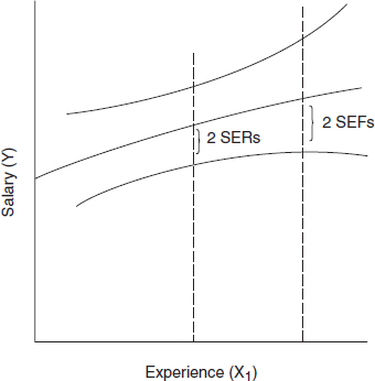
Jane Thompson filed suit in federal court alleging that officials in the police department discriminated against her and a class of other female police officers in violation of Title VII of the Civil Rights Act of 1964, as amended. On behalf of the class, Ms. Thompson alleged that she was paid less than male police officers with equivalent skills and experience. Both plaintiff and defendant used expert economists with econometric expertise to present statistical evidence to the court in support of their positions.
Plaintiff’s expert pointed out that the mean salary of the 40 female officers was $30,604, whereas the mean salary of the 60 male officers was $43,077. To show that this difference was statistically significant, the expert put forward a regression of salary (SALARY) on a constant term and a dummy indicator variable (FEM) equal to 1 for each female and 0 for each male. The results were as follows:
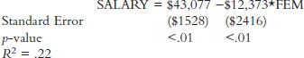
The −$12,373 coefficient on the FEM variable measures the mean difference between male and female salaries. Because the standard error is approximately one-fifth of the value of the coefficient, this difference is statistically significant at the 5% (and indeed at the 1%) level. If this is an appropriate regression model (in terms of its implicit characterization of salary determination), one can conclude that it is highly unlikely that the difference in salaries between men and women is due to chance.
The defendant’s expert testified that the regression model put forward was the wrong model because it failed to account for the fact that males (on average) had substantially more experience than females. The relatively low R2 was an indication that there was substantial unexplained variation in the salaries of male and female officers. An examination of data relating to years spent on the job showed that the average male experience was 8.2 years, whereas the average for females was only 3.5 years. The defense expert then presented a regression analysis that added an additional explanatory variable (i.e., a covariate), the years of experience of each police officer (EXP). The new regression results were as follows:
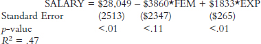
Experience is itself a statistically significant explanatory variable, with a p-value of less than .01. Moreover, the difference between male and female
salaries, holding experience constant, is only $3860, and this difference is not statistically significant at the 5% level. The defense expert was able to testify on this basis that the court could not rule out alternative explanations for the difference in salaries other than the plaintiff’s claim of discrimination.
The debate did not end here. On rebuttal, the plaintiff’s expert made three distinct points. First, whether $3860 was statistically significant or not, it was practically significant, representing a salary difference of more than 10% of the mean female officers’ salaries. Second, although the result was not statistically significant at the 5% level, it was significant at the 11% level. If the regression model were valid, there would be approximately an 11% probability that one would err by concluding that the mean salary difference between men and women was a result of chance.
Third, and most importantly, the expert testified that the regression model was not correctly specified. Further analysis by the expert showed that the value of an additional year of experience was $2333 for males on average, but only $1521 for females. Based on supporting testimonial experience, the expert testified that one could not rule out the possibility that the mechanism by which the police department discriminated against females was by rewarding males more for their experience than females. The expert made this point clear by running an additional regression in which a further covariate was added to the model. The new variable was an interaction variable, INT, measured as the product of the FEM and EXP variables. The regression results were as follows:
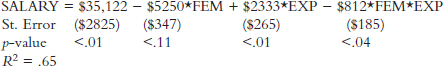
The plaintiff’s expert noted that for all males in the sample, FEM = 0, in which case the regression results are given by the equation
SALARY = $35,122 + $2333*EXP
However, for females, FEM = 1, in which the corresponding equation is
SALARY = $29,872 + $1521*EXP
It appears, therefore, that females are discriminated against not only when hired (i.e., when EXP = 0), but also in the reward they get as they accumulate more and more experience.
The debate between the experts continued, focusing less on the statistical interpretation of any one particular regression model, but more on the model choice itself, and not simply on statistical significance, but also with regard to practical significance.
The following terms and definitions are adapted from a variety of sources, including A Dictionary of Epidemiology (John M. Last et al., eds., 4th ed. 2000) and Robert S. Pindyck & Daniel L. Rubinfeld, Econometric Models and Economic Forecasts (4th ed. 1998).
alternative hypothesis. See hypothesis test.
association. The degree of statistical dependence between two or more events or variables. Events are said to be associated when they occur more frequently together than one would expect by chance.
bias. Any effect at any stage of investigation or inference tending to produce results that depart systematically from the true values (i.e., the results are either too high or too low). A biased estimator of a parameter differs on average from the true parameter.
coefficient. An estimated regression parameter.
confidence interval. An interval that contains a true regression parameter with a given degree of confidence.
consistent estimator. An estimator that tends to become more and more accurate as the sample size grows.
correlation. A statistical means of measuring the linear association between variables. Two variables are correlated positively if, on average, they move in the same direction; two variables are correlated negatively if, on average, they move in opposite directions.
covariate. A variable that is possibly predictive of an outcome under study; an explanatory variable.
cross-sectional analysis. A type of multiple regression analysis in which each data point is associated with a different unit of observation (e.g., an individual or a firm) measured at a particular point in time.
degrees of freedom (DF). The number of observations in a sample minus the number of estimated parameters in a regression model. A useful statistic in hypothesis testing.
dependent variable. The variable to be explained or predicted in a multiple regression model.
dummy variable. A variable that takes on only two values, usually 0 and 1, with one value indicating the presence of a characteristic, attribute, or effect (1), and the other value indicating its absence (0).
efficient estimator. An estimator of a parameter that produces the greatest precision possible.
error term. A variable in a multiple regression model that represents the cumulative effect of a number of sources of modeling error.
estimate. The calculated value of a parameter based on the use of a particular sample.
estimator. The sample statistic that estimates the value of a population parameter (e.g., a regression parameter); its values vary from sample to sample.
ex ante forecast. A prediction about the values of the dependent variable that go beyond the sample; consequently, the forecast must be based on predictions for the values of the explanatory variables in the regression model.
explanatory variable. A variable that is associated with changes in a dependent variable.
ex post forecast. A prediction about the values of the dependent variable made during a period in which all values of the explanatory and dependent variables are known. Ex post forecasts provide a useful means of evaluating the fit of a regression model.
F-test. A statistical test (based on an F-ratio) of the null hypothesis that a group of explanatory variables are jointly equal to 0. When applied to all the explanatory variables in a multiple regression model, the F-test becomes a test of the null hypothesis that R2 equals 0.
feedback. When changes in an explanatory variable affect the values of the dependent variable, and changes in the dependent variable also affect the explanatory variable. When both effects occur at the same time, the two variables are described as being determined simultaneously.
fitted value. The estimated value for the dependent variable; in a linear regression, this value is calculated as the intercept plus a weighted average of the values of the explanatory variables, with the estimated parameters used as weights.
heteroscedasticity. When the error associated with a multiple regression model has a nonconstant variance; that is, the error values associated with some observations are typically high, while the values associated with other observations are typically low.
hypothesis test. A statement about the parameters in a multiple regression model. The null hypothesis may assert that certain parameters have specified values or ranges; the alternative hypothesis would specify other values or ranges.
independence. When two variables are not correlated with each other (in the population).
independent variable. An explanatory variable that affects the dependent variable but that is not affected by the dependent variable.
influential data point. A data point whose deletion from a regression sample causes one or more estimated regression parameters to change substantially.
interaction variable. The product of two explanatory variables in a regression model. Used in a particular form of nonlinear model.
intercept. The value of the dependent variable when each of the explanatory variables takes on the value of 0 in a regression equation.
least squares. A common method for estimating regression parameters. Least squares minimizes the sum of the squared differences between the actual values of the dependent variable and the values predicted by the regression equation.
linear regression model. A regression model in which the effect of a change in each of the explanatory variables on the dependent variable is the same, no matter what the values of those explanatory variables.
mean (sample). An average of the outcomes associated with a probability distribution, where the outcomes are weighted by the probability that each will occur.
mean squared error (MSE). The estimated variance of the regression error, calculated as the average of the sum of the squares of the regression residuals.
model. A representation of an actual situation.
multicollinearity. When two or more variables are highly correlated in a multiple regression analysis. Substantial multicollinearity can cause regression parameters to be estimated imprecisely, as reflected in relatively high standard errors.
multiple regression analysis. A statistical tool for understanding the relationship between two or more variables.
nonlinear regression model. A model having the property that changes in explanatory variables will have differential effects on the dependent variable as the values of the explanatory variables change.
normal distribution. A bell-shaped probability distribution having the property that about 95% of the distribution lies within 2 standard deviations of the mean.
null hypothesis. In regression analysis the null hypothesis states that the results observed in a study with respect to a particular variable are no different from what might have occurred by chance, independent of the effect of that variable. See hypothesis test.
one-tailed test. A hypothesis test in which the alternative to the null hypothesis that a parameter is equal to 0 is for the parameter to be either positive or negative, but not both.
outlier. A data point that is more than some appropriate distance from a regression line that is estimated using all the other data points in the sample.
p-value. The significance level in a statistical test; the probability of getting a test statistic as extreme or more extreme than the observed value. The larger the p-value, the more likely that the null hypothesis is valid.
parameter. A numerical characteristic of a population or a model.
perfect collinearity. When two or more explanatory variables are correlated perfectly.
population. All the units of interest to the researcher; also, universe.
practical significance. Substantive importance. Statistical significance does not ensure practical significance, because, with large samples, small differences can be statistically significant.
probability distribution. The process that generates the values of a random variable. A probability distribution lists all possible outcomes and the probability that each will occur.
probability sampling. A process by which a sample of a population is chosen so that each unit of observation has a known probability of being selected.
quasi-experiment (or natural experiment). A naturally occurring instance of observable phenomena that yield data that approximate a controlled experiment.
R-squared (R2). A statistic that measures the percentage of the variation in the dependent variable that is accounted for by all of the explanatory variables in a regression model. R-squared is the most commonly used measure of goodness of fit of a regression model.
random error term. A term in a regression model that reflects random error (sampling error) that is the result of chance. As a consequence, the result obtained in the sample differs from the result that would be obtained if the entire population were studied.
regression coefficient. Also, regression parameter. The estimate of a population parameter obtained from a regression equation that is based on a particular sample.
regression residual. The difference between the actual value of a dependent variable and the value predicted by the regression equation.
robust estimation. An alternative to least squares estimation that is less sensitive to outliers.
robustness. A statistic or procedure that does not change much when data or assumptions are slightly modified is robust.
sample. A selection of data chosen for a study; a subset of a population.
sampling error. A measure of the difference between the sample estimate of a parameter and the population parameter.
scatterplot. A graph showing the relationship between two variables in a study; each dot represents one subject. One variable is plotted along the horizontal axis; the other variable is plotted along the vertical axis.
serial correlation. The correlation of the values of regression errors over time.
slope. The change in the dependent variable associated with a one-unit change in an explanatory variable.
spurious correlation. When two variables are correlated, but one is not the cause of the other.
standard deviation. The square root of the variance of a random variable. The variance is a measure of the spread of a probability distribution about its mean; it is calculated as a weighted average of the squares of the deviations of the outcomes of a random variable from its mean.
standard error of forecast (SEF). An estimate of the standard deviation of the forecast error; it is based on forecasts made within a sample in which the values of the explanatory variables are known with certainty.
standard error of the coefficient; standard error (SE). A measure of the variation of a parameter estimate or coefficient about the true parameter. The standard error is a standard deviation that is calculated from the probability distribution of estimated parameters.
standard error of the regression (SER). An estimate of the standard deviation of the regression error; it is calculated as the square root of the average of the squares of the residuals associated with a particular multiple regression analysis.
statistical significance. A test used to evaluate the degree of association between a dependent variable and one or more explanatory variables. If the calculated p-value is smaller than 5%, the result is said to be statistically significant (at the 5% level). If p is greater than 5%, the result is statistically insignificant (at the 5% level).
t-statistic. A test statistic that describes how far an estimate of a parameter is from its hypothesized value (i.e., given a null hypothesis). If a t-statistic is sufficiently large (in absolute magnitude), an expert can reject the null hypothesis.
t-test. A test of the null hypothesis that a regression parameter takes on a particular value, usually 0. The test is based on the t-statistic.
time-series analysis. A type of multiple regression analysis in which each data point is associated with a particular unit of observation (e.g., an individual or a firm) measured at different points in time.
two-tailed test. A hypothesis test in which the alternative to the null hypothesis that a parameter is equal to 0 is for the parameter to be either positive or negative, or both.
variable. Any attribute, phenomenon, condition, or event that can have two or more values.
variable of interest. The explanatory variable that is the focal point of a particular study or legal issue.
References on Multiple Regression
Jonathan A. Baker & Daniel L. Rubinfeld, Empirical Methods in Antitrust: Review and Critique, 1 Am. L. & Econ. Rev. 386 (1999).
Gerald V. Barrett & Donna M. Sansonetti, Issues Concerning the Use of Regression Analysis in Salary Discrimination Cases, 41 Personnel Psychol. 503 (2006).
Thomas J. Campbell, Regression Analysis in Title VII Cases: Minimum Standards, Comparable Worth, and Other Issues Where Law and Statistics Meet, 36 Stan. L. Rev. 1299 (1984).
Catherine Connolly, The Use of Multiple Regression Analysis in Employment Discrimination Cases, 10 Population Res. & Pol’y Rev. 117 (1991).
Arthur P. Dempster, Employment Discrimination and Statistical Science, 3 Stat. Sci. 149 (1988).
Michael O. Finkelstein, The Judicial Reception of Multiple Regression Studies in Race and Sex Discrimination Cases, 80 Colum. L. Rev. 737 (1980).
Michael O. Finkelstein & Hans Levenbach, Regression Estimates of Damages in Price-Fixing Cases, Law & Contemp. Probs., Autumn 1983, at 145.
Franklin M. Fisher, Multiple Regression in Legal Proceedings, 80 Colum. L. Rev. 702 (1980).
Franklin M. Fisher, Statisticians, Econometricians, and Adversary Proceedings, 81 J. Am. Stat. Ass’n 277 (1986).
Joseph L. Gastwirth, Methods for Assessing the Sensitivity of Statistical Comparisons Used in Title VII Cases to Omitted Variables, 33 Jurimetrics J. 19 (1992).
Note, Beyond the Prima Facie Case in Employment Discrimination Law: Statistical Proof and Rebuttal, 89 Harv. L. Rev. 387 (1975).
Daniel L. Rubinfeld, Econometrics in the Courtroom, 85 Colum. L. Rev. 1048 (1985).
Daniel L. Rubinfeld & Peter O. Steiner, Quantitative Methods in Antitrust Litigation, Law & Contemp. Probs., Autumn 1983, at 69.
Daniel L. Rubinfeld, Statistical and Demographic Issues Underlying Voting Rights Cases, 15 Evaluation Rev. 659 (1991).
The Evolving Role of Statistical Assessments as Evidence in the Courts (Stephen E. Fienberg ed., 1989).


