
In this chapter, we discuss the recent research that used panel data and methods to examine whether the death penalty has a deterrent effect on homicide and if so, the size of this effect. As noted in Chapter 1, “panel data” and “panel methods” refer to data from many geographic locations followed over time—usually annual state-level data—and a particular set of multiple regression methods. The annual state data include all states, and the time periods covered are typically from the late 1970s (post-Gregg) through the late 1990s or into the 2000s. Over this time period, there have been variations in the frequency of death penalty sentences, executions, and the legal availability of the death penalty. With these types of data, the strategy for identifying an effect of the death penalty on homicides has been, roughly speaking, to compare the variation over time in the average homicide rates among states that changed their death penalty sanctions versus those that did not.
This chapter assesses the extent to which the research using panel data is informative on the question of whether and how much the death penalty has a deterrent effect on homicide. For this assessment, we compare the data and methods used in this literature with those that would be available from an ideal randomized experiment (see Chapter 3). The purpose of this exercise is to clarify the challenges that face researchers using panel methods to study the death penalty and deterrence. We then assess the extent to which this research overcomes these challenges.
This literature is striking in the similarity of the data and methods used across studies and the diversity of the results. Given this diversity of results
across and in some cases within studies, a central task for this committee is to assess the validity of the models used in the studies.
We begin the chapter by describing the key features of the studies we reviewed and giving a brief overview of their data and methods. We then discuss the primary challenges to researchers using panel data and methods to inform the question of whether the death penalty affects the homicide rate: the difficulty in measuring changes over time in the relevant sanction policies for homicide and the difficulties in establishing that any changes in homicides that are concurrent with changes in the death penalty are caused by those changes in the death penalty and not vice versa or by other factors that affect both—such as other sanctions for murder. We conclude with our assessment of the informativeness of the panel research.
We begin our review of the panel research by briefly describing the regression models used in the studies. Our intention with this description is to establish the extent to which the methods are largely consistent across studies, as context for understanding the particular dimensions on which the studies differ.
The panel research makes use of multiple regression models involving “fixed effects” that take the following form:
![]()
where yit is the number of homicides per 100,000 residents in state i in year t, f(Zit) is an expected cost function of committing a capital homicide that depends on the vector of death penalty or other sanction variables Zit with corresponding parameter γ measuring the effect of the death penalty on the homicide rate. Importantly, this effect is assumed to be homogeneous across states i and years t.
A primary benefit of panel data is that one observes homicide and execution rates in the 50 states over many years. This allows researchers to effectively account for unobserved features of the state or of the time period that might be associated with both the application of the death penalty and the homicide rate. Some states, for example, might have unobserved social norms that lead to higher (or lower) execution rates and lower (or higher) rates or homicide: Texas is arguably different than Massachusetts in this regard. The panel data model in Equation (4-1) accounts for some of these differences with a state-specific intercept parameter, αi, referred to as a state fixed effect, that allows the mean homicide rate to vary additively
by state, and a time-specific intercept, βit, referred to as a time fixed effect, that allows the mean homicide rate to vary additively over time. These fixed effects account for unobserved factors that are state specific but fixed across time, such as the social norms that make Texas different than Massachusetts, and factors that are year specific but apply to all states, such as macroeconomic events that may affect homicide rates across the country. In addition to these fixed effects, some of the researchers also include state-specific linear time trends that allow each state’s homicide rate trend to vary (linearly) from the year-to-year national fluctuations.
The literature also includes a set of covariates, Xit, that are intended to control for additional factors that may vary with both state and year. These sets of covariates are largely similar across studies and include economic indicators, such as the unemployment rate and real per capita income; demographic variables, such as the proportion of the state’s population in each of several age groups; the proportion of the state’s population that is black; and the proportion of the state’s population that reside in urban areas. The covariates also include health and policy variables, such as the infant mortality rate, the legal drinking age, and the governor’s party affiliation; and crime, policing, or sanctioning variables, such as the number of prisoners per violent crime.
Finally, εit is a random variable that accounts for the unobserved factors determining the homicide rate.1 Researchers make two general assumptions about the relationship between the death penalty variables, Zit, and εit. The most common assumption is that the death penalty, as measured by the variable Zit, is statistically independent of the unobserved factors that determine homicide, as it would be in an ideal randomized experiment. An alternative route is to assume that there is some covariate, termed an instrumental variable, that is independent of εit but not of the death penalty.
The Studies, Their Characteristics, and the Effects Found
Table 4-1 lists the studies reviewed in this chapter and a few of their key characteristics, and briefly notes each one’s results.2 This list does not
__________________
1 In estimating these models, the data are typically weighted by state population.
2 One characteristic that is not highlighted in Table 4-1 is the choice of outcome variable, yit. All of the studies listed in the table and reviewed in this chapter focused on the overall homicide rate (or the log-rate). However, there are a few studies in the panel data literature that examined different outcome measures. Most notably, Fagan, Zimring, and Geller (2006) focused on all capital murders, and Frakes and Harding (2009) examined child murders which, depending on the state and year, may or may not be death penalty eligible. Otherwise, the key characteristics of these two studies are similar to the ones reviewed in this chapter. Interestingly, although both studies focused on the impact of the death penalty on capital eligible murders, Fagan, Zimring, and Geller found no evidence that the death penalty deters murder,
TABLE 4-1 Panel Studies Reviewed
| Study | Legal Status | Intensity of Use | Use of an Instrument | Results: Signa and Significanceb of Point Estimates | |
| Berk (2005) | N | Y | N | All possible results | |
| Cohen-Cole et al. (2009) | Y | Y | Y | All possible results | |
| Donohue and Wolfers (2005, 2009) | Y | Y | Y | All possible results | |
| Dezhbakhsh and Shepherd (2006) | Y | Y | N | –** | |
| Dezhbakhsh, Rubin, and Shepherd (2003)c | Y | Y | Y | –**; and –NS | |
| Katz, Levitt, and Shustorovich (2003) | N | Y | N | –**; –NS; and +NS | |
| Kovandzic, Vieraitis, and Boots (2009) | Y | Y | N | –NS; +NS | |
| Mocan and Gittings (2003) | Y | Y | N | –**; and –NS | |
| Mocan and Gittings (2010) | N | Y | N | –**; and –NS | |
| Zimmerman (2004) | N | Y | Y | –*; and –NS | |
aSign of the estimated coefficients: –, the estimated effect of capital sanctions on homicide is negative, indicating a deterrent effect; +, the estimated effect of capital sanctions on homicide is positive, indicating a brutalization effect.
bStatistical significance levels: NS, no statistical significance at p = 0.05; *, p < 0.05; **, p < 0.01.
cDezhbakhsh, Rubin, and Shepherd (2003) estimate 55 different panel data regression models. In 49 of the models, the estimated effect of capital sanctions on homicide is negative and statistically significant; in 4, the estimates are negative and insignificant; and in 2, the estimates are positive and insignificant.
include every study of deterrence using panel data, but instead provides information on a set of influential studies that use the different approaches found in the research and that draw a wide range of different conclusions. Studies designed to illustrate the fragility of the results reports in the literature, namely, Donohue and Wolfers (2005, 2009) and Cohen-Cole et al. (2009), apply the same basic models and thus are included in our review.
The first study characteristic is how researchers specify the expected cost function of committing a capital homicide f(Zit). At the most basic level, studies seek to determine the effect of changes in the legal status of the death penalty, changes in the intensity with which the death penalty is applied, or both. Most studies evaluated the intensity of use, but some also focused on the legal status of the death penalty. The specification of the death penalty variables in the panel models varies widely across the research and has been the focus of much debate. The different specifications assume that quite different aspects of the sanction regime are salient for would-be murderers. The research has demonstrated that different death penalty sanction variables, and different specifications of these variables, lead to very different deterrence estimates—negative and positive, large and small, both statistically significant and not statistically significant.
The second characteristic of interest is whether the death penalty measure is assumed to be randomly applied after controlling for the observed covariates and the fixed effects. The choice of whether or not to use instrumental variables, and the particular variables selected, has led to contentious differences in model assumptions invoked across the literature. In most of the studies, the researchers have assumed that the death penalty is unrelated to the unobserved factors associated with the homicide rate. That is, the unobserved factors, εit, are not associated with the death penalty sanctions. Studies using this independence assumption have drawn conflicting conclusions (see Table 4-1) with some reporting statistically significant evidence in favor of a deterrence effect, many others finding that capital punishment has a negative but statistically insignificant association with homicide, and a few others reporting evidence in favor of a brutalization effect, that capital punishment increases homicide.
Dezhbakhsh, Rubin, and Shepherd (2003) and Zimmerman (2004) argue that death penalty sanctions are likely to be correlated with unobserved determinants of homicide, and instead propose using instrumental variables to provide variation in the risk perceptions of potential murderers that is separable from the effects of all of the unobserved factors. The results of
__________________
and Frakes and Harding reported substantial deterrent effects. Our review does not consider the choice of the outcome variable: although this choice may have important implications for inference, these issues are secondary relative to the more fundamental issues covered in this chapter.
studies that do not use such instrumental variables vary from those that do, and the results of studies that use different instrumental variables vary from each other.
The fact that the estimated effects of the death penalty on homicide are sensitive to the different data and modeling assumptions used is not surprising. Deterrence estimates from the panel models depend on state changes over time in the legal status of the death penalty or the intensity with which the death penalty is applied. Since the moratorium was lifted, such changes have been few and far between (see Chapter 2). Because of the way in which the death penalty has been implemented in the United States in the last 30 years, no executions occur in most states in most years (86 percent of state-year observations), and when there are any, the number is almost always very low. In addition, the executions that do occur are concentrated in particular states, with Texas carrying out executions an order of magnitude more often than any other state. There also tends to be little variability for states over time in their numbers of or rates of executions and whether they legally allow executions. Only 11 states experienced one or more changes in legal status of the death penalty after the national moratorium was lifted. Overall, in recent decades in the United States the death penalty has been a rare practice that is concentrated in a few places.
Not only is there low variability in the application of the death penalty, there are only a small number of state-year observations that exhibit large variations in homicide rates over time. Figure 4-1 illustrates a partial regression plot with a death penalty sanction measure on the horizontal axis and the homicide rate on the vertical axis (adjusted for state and year fixed effects and typical covariates). This plot reflects the data, covariates, and specification used by Kovandzic, Vieraitis, and Boots (2009).3 In displaying these regression results, the committee is not endorsing this or any other particular study.4 Instead, our purpose is to illustrate how outlier or influential observations may affect regression results. Since the effect of the death penalty is estimated as the slope of the ordinary least squares regression line between the bulk of the data near zero and the location of the small set of influential values, the estimates in the research studies can vary widely (Berk, 2005). For example, if the particular state-year observations that are influential depend on the death penalty intensity measure used, then the slope of the regression line will vary with this measure. If one believes in the validity of the underlying model applied in Figure 4-1, then the outlier
__________________
3 The execution measure is computed using the number of executions the year before the period year divided by the number of death sentences 7 years prior to the period year. For full model specification, see Figure 4-1 notes in the figure caption.
4 In particular, we note that alternative but similar specifications result in a positive sloping, rather than a negative sloping line.
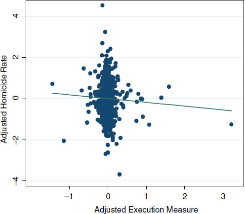
FIGURE 4-1 Illustration of influential data points.
NOTES: The plot reflects the data, covariates, and specification used by Kovandzic, Vieraitis, and Boots (2009), Table 3, Model 6 with the addition of two common sanction variables: death sentences divided by homicide arrests 2 years prior and homicide arrests divided by homicides. These additional variables required a measure of arrests for homicide, which was obtained from J. Wolfers’ web page and was not available for years after 1998.
The horizontal axis represents the adjusted execution measure (residuals of execution measure regressed on all the rest of the regressors in the model). The execution measure is defined as the number of executions the prior year per number of death sentences 7 years prior, with missing values set to zero.
The vertical axis represents the adjusted homicide rate (residuals of the homicide rate regressed on all the regressors except the execution rate variable). The homicide rate is homicides per 100,000 residents. The regression was run on data for 1984-1998, weighted by state population share, and standard errors were clustered by state.
The coefficient of the ordinary least squares line between these two sets of adjusted variables—and hence the coefficient on the execution measure in the multiple linear regression of homicide rates on the execution measure and all covariates—is –0.183 (p = 0.173).
SOURCES: Data from T.V. Kovandzic (personal communication) and J. Wolfers. Wolfers’ data are available at http://bpp.wharton.upenn.edu/jwolfers/DeathPenalty.shtml.
observations are informative. But if there is uncertainty about the validity of the model, the outliers can make the estimates highly sensitive to the underlying assumptions.
As noted in Chapter 2, the infrequency of executions does not mean that there is insufficient variation in the data to detect the effect of capital punishment. In fact, as shown in Table 4-1 (above), there is no shortage of statistically significant results reported in the literature. Rather, the problem is that inferences on the impact of the death penalty rest heavily on unsupported assumptions.
SPECIFYING THE EXPECTED COST OF COMMITTING A CAPITAL HOMICIDE: f(Zit)
In light of the variability in the estimated effects of the death penalty on homicide, a central question is whether the correct specification is being used and can be identified. We evaluate this question below by first focusing on measures of the perceived cost of murder and then taking up more generic issues associated with the panel data models in equation (4-1).
A vital component to evaluating the effect of the death penalty on homicide is to properly specify the expected cost function, f(Zit), in Equation (4-1). Yet, researchers have failed to measure the relevant sanction regime and have relied on seemingly ad hoc measures of the relevant sanction probabilities.
What is the relevant treatment? Researchers have struggled to clearly specify and measure the incremental cost of a particular sanction policy. As noted in Chapter 3, there is little information on the sanction regime, and thus the counterfactual policy of interest. In particular, the research aims to determine the effect of an increase (or decrease) in the risk of receiving the death penalty or being executed relative not to no sanction, but rather relative to the other common sanctions for murder—lengthy prison sentences (with or without the possibility of parole). Moreover, these other aspects of the sanction regime may be changing over time, and any changes in the risks of the death penalty have to be evaluated relative to the varying but always higher risks associated with prison sentences. Two mechanisms that could plausibly create associations between changes in death penalty and prison sentence sanctions for homicide are the plea bargaining process, through which the threat of the death penalty may change the likelihood of sentences of different lengths, including life without parole, and the punitiveness of a state’s culture, which influences the severity of the capital and noncapital aspects of the sanction regime.
None of the studies we reviewed made any use of information on other sanction risks for murder or the ways in which they may be changing over time. For this reason, it is not possible to tell if any “treatment” effects
found in these models are due to death penalty sanction changes or to changes in other more frequently used sanctions that are part of a state’s sanction regime for homicide. If changes in the death penalty are part of a larger “law and order” program, then concurrent changes in other much more heavily used sanctions could be at the root of any associated change in homicide rates.
A related problem in specifying a cost function is the ad hoc and inconsistent measures of subjective sanction probabilities. How do potential offenders measure the expected cost of committing a capital offense? The difficulty in answering this question stems from two interrelated problems: first, there is little information on how offenders perceive the relevant probabilities of arrest, conviction, and execution; and second, in practice, these probabilities may be difficult to measure.
In the studies we reviewed, one or both of just two features of the death penalty are assumed to be salient for deterring homicide: the legal status of the death penalty (in each state and year) and what are described as measures of the intensity with which the death penalty is applied (in each state and year). A variety of different and complex temporal structures are used to measure the probabilities of arrest, death sentence, and execution.
Consider, for example, the specifications used for variables described as the risk of execution given a death sentence:
• the number of executions in the prior year (prior to the current year’s homicide rate);
• the number of executions in the prior year divided by the number of death sentences in the same prior year (or a variant, using a 12-month moving average of these counts for both the numerator and denominator);
• the number of executions in the current or prior year divided by the number of death sentences in an earlier prior year (3, 4, 5, 6, and 7 years prior have all been implemented and similar specifications using executions from the first three quarters of the current year and last quarter of prior year divided by death sentences 6 years prior);
• the number of executions in the prior year divided by the number of death row inmates in the prior year;
• the number of executions in the current year divided by the number of homicides in the prior year;
• the number of executions in the prior year divided by the number of prisoners in the prior year (or 2 or 3 years prior); and
• the number of executions in the prior year divided by the population of the state in the prior year.
There is no empirical basis for choosing among these specifications, and there has been heated debate among researchers about them, particularly on the number of years that should be lagged for the numerator and, even more so, for the denominator in order to best correspond to the relevant risk of execution given a death sentence in each state and year.
This debate, however, is not based on clear and principled arguments as to why the probability timing that is used corresponds to the objective probability of execution, or, even more importantly, to criminal perceptions of that probability. Instead, researchers have constructed ad hoc measures of criminal perceptions. Consequently, the results have proven to be highly sensitive to the specific measures used. Donohue and Wolfers (2005) find, for example, that when reanalyzing the results in Mocan and Gittings (2003), using a 7-year lag implies that the death penalty deters homicide (4.4 lives saved per execution) but using a 1-year lag implies that the death penalty increases the number of homicides (1.2 lives lost per execution). Donohue and Wolfers (2005) question whether would-be murderers are aware of the number of death sentences handed down 7 years prior. Responding to these concerns, Mocan and Gittings (2010) argue that because executions do not take place the same year as a sentence is imposed, models with a 1-year lag are meaningless.
Whether any of these measures accurately reflect the relevant risk probabilities is uncertain. The basic problem is that little is known about how those who may commit murder perceive the sanctions for this crime. If the death penalty is going to have an effect on the behavior of this group, it is their perceptions of the sanction regime for murder that matter. It is not known whether the current legal status of the death penalty is salient to potential murderers; other relevant factors could include how often the legal status of the death penalty has changed in recent years and the presence of high-profile cases, which create greater awareness of the legality of the death penalty in a state. Similarly, it is not known whether specific state and year information is salient to potential murderers; no evidence or theory is presented in the studies we reviewed to argue that the particular measures are valid or that alternative measures—such as executions in surrounding states or in one’s own county or executions in the last 5 years or the last 3 months—are not equally valid. As potential murderers may be attempting to predict the effective sanction regime several or many years into the future, when they might be sentenced or executed, it is particularly unclear what the relevant geographic or time horizon is for obtaining a salient measure.
Suppose that when deciding whether to commit a crime, potential murderers weigh the benefits and risks that committing murder may bring them along with the likelihood of those benefits or risks occurring. In this setting, the probability of being sentenced to death and henceforth being
executed are theorized to be among these perceived risks. The sanction risks are necessarily based on the individual’s perceptions. Either implicitly or explicitly, researchers in this field typically make an additional assumption that the risk perceptions of potential murderers are accurate and thus the perceived risks of receiving a death sentence, being executed, or being executed within a particular time period, are equivalent to the objective measures of these risks. The accuracy of this assertion that the risk perceptions of potential murderers are correct is questionable. There is no clear enforcement mechanism or learning process that would create such accuracy over time in potential murderers’ perceptions of the risk of incurring the death penalty.
Even if potential murderers’ risk perceptions are accurate, researchers must carefully specify the probabilities that might affect behavior and must confront the practical difficulties involved in measuring the relevant probabilities. The studies to date, however, have failed to address either of these issues. Because the post-Gregg panel research has not developed models based on the potential offender’s decision problem, the studies may mis-specify the relevant risk probabilities.
Much of this research considers how different conditional probabilities—say, the probability of execution given capital sanctions—each separately affects behavior (see, e.g., Dezhbakhsh, Rubin, and Shepherd, 2003). Yet, in standard decision models in which potential offenders weigh the uncertain benefits and costs of committing a crime, the joint probability of execution, capital sanctions, and arrests are germane. In this expected utility framework, Durlauf, Navarro, and Rivers (2010) show that the effect of the conditional probability of execution given a death sentence cannot be understood separately from the effects of the conditional probability of being caught and being sentenced to death if caught. Moreover, under a rational choice assumption, what will matter is the expected execution rate at time t + 6, which is not necessarily equal to the t – 6 years used in the literature.
Aside from this important issue of modeling and functional form, researchers also encounter practical obstacles in measuring the objective risks. Consider the risk of being executed given a death sentence, the risk that has been most focused on in the research, and consider how this risk could be objectively measured and updated each year for those in each state, as is assumed relevant in these models. In 1977, the first full year after the Gregg decision, 31 states provided the legal authority to impose the death penalty. In 1977, there were no data on the actual use of the death penalty in any state to create an estimate of the risk of execution. Some people might have predicted that Texas would be more vigorous in its actual use of the death penalty than California or Pennsylvania, but there were as yet no data to confirm such a prediction. Thus, it is unclear what the objective risk of receiving a death sentence or consequently being executed was in
any state for which the death penalty was legal in 1977. Only over time could an objective risk be based on data. Thus, over time one would expect divergent risks to develop in different states as data on the actual use of the death penalty in each state accumulated.
The process of forming and revising objective measures of the risks associated with the death penalty, however, would then be complicated by additional factors. One is that the volume of data on death sentences and executions available for calculating estimates of risk depends on the size of the state. By various measures of execution risk reported in Chapter 2, Delaware was at least as aggressive in its use of the death penalty as Texas. However, over the period from 1976 to 2000, Delaware sentenced 28 people to death and carried out 11 executions, while Texas sentenced 753 people to death and carried out 231 executions. Thus, potential murderers have far more data on the actual practice of capital punishment each year in Texas than in Delaware. As a consequence, even for well-informed potential murderers living in states with similar sanction regimes, one would expect sanction risk perceptions to evolve along different paths that would depend, among other things, on the size of the state.
Perhaps in an environment in which sanction regimes were plausibly stable, the objective risk of execution could be precisely estimated even in small states with low murder rates. However, sanction regimes do not appear to be uniformly stable in large states for which it is feasible to obtain precise measures of year-to-year variation. Indeed, it is changes in the sanction regime for murder that the panel models use to inform their estimates of deterrence. Moratoriums and commutations may signal changes in regimes, particularly when accompanied by high-visibility announcements such as that by former Illinois Governor George Ryan in 2000. As noted in Chapter 2, Texas appears to have shifted to a higher intensity execution sanction regime during the 1990s. Thus, in an environment in which sanction regimes are changing, the value of older data in forming a correct estimate of the prevailing sanction regime deteriorates. Moreover, the value of current data in forming a correct estimate of the future sanction regime also deteriorates. This forecast is particularly relevant as those considering murder now would face the sanction regime of the state in which the homicide is prosecuted some significant time in the future. These factors raise the question of whether year-to-year variation in a measure, such as the number of people executed in a state, has any bearing on the risk of execution for someone committing a murder today. Overall, the degree to which this, or other proposed measures of execution risk, predicts later executions has not been established.
To illustrate the problems associated with these different measures, consider using the number of executions in a state 1 year prior to the
year in which the homicide rate is measured divided by the number of death sentences in that state 7 years earlier. Those at risk for execution in any particular year are all those on death row at some point in that year. Those who were sentenced to death 7 years earlier could be executed at any time after their sentence, with different probabilities of being executed in each year based on the particulars of their crime, the appeals process, their health, the current governor, etc. In the early years after the national death penalty moratorium ended, on a national level, those who were executed had spent an average of 6-7 years on death row (Snell, 2010). There are several problems with using this information to justify lagging the denominator of a risk of execution measure by 7 years. First, only 15 percent of those sentenced to death in the United States since 1977 have been executed, with close to 40 percent leaving death row for other reasons (vacated sentences or convictions, commutations, a successful appeal, or death by other causes), and 45 percent are still on death row (Snell, 2010). Moreover, these figures vary substantially across states and over time.
Table 4-2 displays the number of inmates removed from death row in each state by the reasons for removal. First, there is substantial variation in the execution rates across states. For example, of the 150 people in Virginia sentenced to death from 1973 to 2009, 105—70 percent—have been executed. In contrast, in North Carolina, only 8 percent of the 528 people sentenced to death have been executed. Not only do these rates vary across states, but they also vary over time (see, e.g., Cook, 2009). Clearly, the number of years those executed have spent on death row is not an accurate measure of the number of years those on death row will spend there before they are executed, if they are ever executed. Second, the time spent on death row by those executed has varied over time at the national level, and it varies considerably by state (Snell, 2010). Third, no evidence has been given or arguments made to suggest that death sentences that come to some resolution earlier than others are indicative of the resolution for death sentences that have not yet come to resolution. Thus, using a fixed number of years of lag between those sentenced and those executed means that for many states and years this lag will have an uncertain relationship to the objective risk of execution given a death sentence.
The fact that there is a mismatch between the numerator and denominator in the models used is perhaps best illustrated by the many state-year cases in which there are one or more executions the prior year but there were no death sentences imposed 7 years earlier. Researchers have made a variety of ad hoc removals or substitutions for these undefined cases including: replace with zero or treat as missing (Kovandzic, Vieraitis, and Boots, 2009); numerator set to zero regardless of denominator and non-zero numerator and zero denominator considered missing at random (Donohue and Wolfers, 2005; Mocan and Gittings, 2003, 2010); replace with most
TABLE 4-2 Death Sentences and Removals, by Jurisdiction and Reason for Removal, 1973-2009
| Jurisdiction | Total Sentenced to Death, 1973-2009 | Removals | Sentence or Conviction Overturned | Sentence Commuted | Other Removals | Under Sentence of Death, December 31, 2009 | |
| Executed | Died | ||||||
| U.S. Total | 8,115 | 1,188 | 416 | 2,939 | 365 | 34 | 3,173 |
| Federal | 65 | 3 | 0 | 6 | 1 | 0 | 55 |
| Alabama | 412 | 44 | 31 | 135 | 2 | 0 | 200 |
| Arizona | 286 | 23 | 14 | 110 | 7 | 1 | 131 |
| Arkansas | 110 | 27 | 3 | 38 | 2 | 0 | 40 |
| California | 927 | 13 | 73 | 142 | 15 | 0 | 684 |
| Colorado | 21 | 1 | 2 | 15 | 1 | 0 | 2 |
| Connecticut | 13 | 1 | 0 | 2 | 0 | 0 | 10 |
| Delaware | 56 | 14 | 0 | 25 | 0 | 0 | 17 |
| Florida | 977 | 68 | 53 | 447 | 18 | 2 | 389 |
| Georgia | 320 | 46 | 16 | 147 | 9 | 1 | 101 |
| Idaho | 42 | 1 | 3 | 21 | 3 | 0 | 14 |
| Illinois | 307 | 12 | 15 | 96 | 156 | 12 | 16 |
| Indiana | 100 | 20 | 4 | 54 | 6 | 2 | 14 |
| Kansas | 12 | 0 | 0 | 3 | 0 | 0 | 9 |
| Kentucky | 81 | 3 | 6 | 35 | 2 | 0 | 35 |
| Louisiana | 238 | 27 | 6 | 114 | 7 | 1 | 83 |
| Maryland | 53 | 5 | 3 | 36 | 4 | 0 | 5 |
| Massachusetts | 4 | 0 | 0 | 2 | 2 | 0 | 0 |
| Mississippi | 190 | 10 | 5 | 112 | 0 | 3 | 60 |
| Missouri | 182 | 67 | 10 | 52 | 2 | 0 | 51 |
| Montana | 15 | 3 | 2 | 6 | 2 | 0 | 2 |
| Nebraska | 32 | 3 | 4 | 12 | 2 | 0 | 11 |
| Nevada | 147 | 12 | 15 | 36 | 4 | 0 | 80 |
| New Hampshire | 1 | 0 | 0 | 0 | 0 | 0 | 1 |
| New Jersey | 52 | 0 | 3 | 33 | 8 | 8 | 0 |
| New Mexico | 28 | 1 | 1 | 19 | 5 | 0 | 2 |
| New York | 10 | 0 | 0 | 10 | 0 | 0 | 0 |
| North Carolina | 528 | 43 | 21 | 297 | 8 | 0 | 159 |
| Ohio | 401 | 33 | 20 | 168 | 15 | 0 | 165 |
| Oklahoma | 350 | 91 | 12 | 165 | 3 | 0 | 79 |
| Oregon | 58 | 2 | 2 | 23 | 0 | 0 | 31 |
| Pennsylvania | 399 | 3 | 24 | 148 | 6 | 0 | 218 |
| Rhode Island | 2 | 0 | 0 | 2 | 0 | 0 | 0 |
| South Carolina | 203 | 42 | 5 | 98 | 3 | 0 | 55 |
| South Dakota | 5 | 1 | 1 | 1 | 0 | 0 | 2 |
| Tennessee | 221 | 6 | 15 | 105 | 4 | 2 | 89 |
| Texas | 1,040 | 447 | 38 | 167 | 56 | 1 | 331 |
| Jurisdiction | Total Sentenced to Death, 1973-2009 | Removals | Sentence or Conviction Overturned | Sentence Commuted | Other Removals | Under Sentence of Death, December 31, 2009 | |
| Executed | Died | ||||||
| Utah | 27 | 6 | 1 | 9 | 1 | 0 | 10 |
| Virginia | 150 | 105 | 6 | 14 | 11 | 1 | 13 |
| Washington | 38 | 4 | 1 | 25 | 0 | 0 | 8 |
| Wyoming | 12 | 1 | 1 | 9 | 0 | 0 | 1 |
| Percentage | 100 | 14.6 | 5.1 | 36.2 | 4.5 | 0.4 | 39.1 |
NOTE: Some inmates executed since 1977 or currently under sentences of death were sentenced prior to 1977. For those inmates sentenced to death more than once, the numbers are based on the most recent death sentence.
SOURCE: Snell (2010), Table 20.
recent defined ratio (Zimmerman, 2004). These (and other) ad hoc adjustments highlight the general problem that the people who were sentenced to death 7 years earlier may be executed before or after the year in which executions are counted, and they are not the only people at risk for being executed in the current or prior year. Overall, the interpretation of this ratio is not clear at all, whether the denominator is lagged any particular number of years, and its relevance to the objective risk of execution for each state and year, let alone to the risk perceptions of potential murderers, is highly questionable.
Basing execution risk measures only on data on executions that have actually been carried out, as has been done in the research being discussed, could result in a serious underestimate of the eventual probability of execution for those given a death sentence. In addition, this fact raises serious questions about whether the risk of ever being executed after a death sentence is the most salient measure or whether additional information is salient, such as measures that consider expected time to death, expected living conditions while on death row, and in comparison, expected time to death during a long prison sentence and conditions while in prison in that state. (Of course, one can only speculate about which, if any, of these variables is salient for potential murderers.)
These many complications make clear that even with a concerted effort by dedicated researchers to assemble and analyze relevant data on death sentences and executions, assessment of the actual and changing objective risk of execution that faces a potential murderer is a daunting challenge. Given the obstacles to obtaining an objective measure of this risk, the committee does not find any of the measures used in the studies to be credible measures of the objective risk of execution given a death sentence. We also reiterate that it is not known whether there is a relationship between any of these measures or any more credible objective measure of execution risk, and the execution risk as perceived by potential murderers.
The conceptual and measurement concerns raised thus far, which are somewhat unique to studies on the effects of the death penalty on homicides, make it difficult to even to envision how one could draw valid inferences on the deterrent effect using the existing data. There is a complete lack of basic information on the noncapital component of the sanction regime, on how offenders perceive sanction risks, and on how to accurately measure those risks.
Even if these measurement problems are some day fully addressed, all studies using observational data must also address the counterfactual outcomes problem that arises because the data cannot reveal the outcome
that would occur if the death penalty had not been applied in treatment states and had been applied in control states. The data alone cannot reveal the effect of the death penalty. Rather, researchers must combine data with assumptions.
In the studies we reviewed, variations of the model in Equation 1 have been used to identify the impact of the death penalty on homicide. In this section, we consider the credibility of the four assumptions that have been applied in this literature: (1) that the death penalty measures are independent of the unobserved factors influencing homicide; (2) that certain observed covariates, called instrumental variables, are correlated with the death penalty but not with the unobserved factors that influence homicide; (3) that the effect of the death penalty is the same for all states and years; and (4) that the sanction regimes of adjacent states do not have any bearing on the effect of the death penalty in a particular state. We begin with a brief discussion of the benefits of random assignment.
As discussed in Chapter 3, random assignment of treatment to large samples of subjects leads the distributions of all other characteristics of treatment and control subjects, whether observed or unobserved, to be approximately the same across the two groups. With small samples of subjects, this feature will hold on average, meaning that if a given set of subjects is repeatedly randomly assigned to treatment or control conditions, then the features of the subjects over all possible treatment groups and all possible controls groups would be exactly equal. In any particular randomization, however, there may be some features that differ by chance for the subjects in the treatment condition and those in the control condition.
This “balancing” of the characteristics of treatment and control subjects justifies the attribution of any difference in outcomes between the treatment and control groups to the treatment and not to other factors that may differ between the treatment and control subjects. Without randomization, the threat of misattributing the cause of any observed differences in outcomes to the treatment when it is actually due to other factors that differ between the groups is always present. In the remainder of this section we focus on the specific challenges this concern raises with regard to the death penalty and deterrence research, discuss the methodological strategies proposed to overcome these challenges, and assess whether these strategies have been successful.
In research on the death penalty and deterrence, the sanction regime for murder (including the legal status of the death penalty and the intensity with which the death penalty is applied) is, for obvious reason, not randomly assigned to state-by-year units. Hence, the possibility is present
that other factors may be the actual causes of any changes seen in homicide rates. Mechanically, what is required for this misattribution to occur is for death penalty changes to occur at similar times and places as changes in the true underlying causal factors. An example is a shift to a political leader with a “law and order” approach, which could both increase death-penalty-related risks and increase the perceived or actual arrest rates, either or both of which could bring down the homicide rate.
Two methodological strategies are used to try to identify changes in the homicide rate that are caused by changes in the sanction regime for murder and not by other factors. The first methodological strategy is a fixed effect multiple regression (described above), in which fixed state and year effects are used to account for unobserved determinants of homicide. Given these fixed effects, researchers assume that the death penalty measures are statistically independent of the unobserved determinants of homicide, as would be the case in a randomized experiment. The second methodological strategy is to add an instrumental variables analysis to the fixed effect multiple regression models.
The fixed effects multiple regression models rely on state level variation in death penalty measures over time to attempt to identify a causal effect of death-penalty-related changes on homicide after controlling for the effects of the other variables in the models. But even if one provisionally assumes that the death penalty measures used in these models are correctly specified (i.e., are the salient factors for potential murderers), that the state-year unit is the unit at which potential murderers are assessing death-penalty-associated risks, and that the specification of all other variables and of the functional form of the model are correct, additional strong assumptions are still required for panel models to deliver estimates of a deterrent effect of the death penalty.
In the fixed effect models, states that do not apply the death penalty sanction are used to estimate the missing counterfactual for states that do experience different death penalty sanction levels. This approach identifies a causal effect only if there are no other factors besides the death penalty causing homicide rates to change differently in states that do and do not experience changes in death penalty sanctions. Many such factors may well exist—such as changes in economic conditions, crime rates, public perceptions or political regimes—and there is no reason to believe that these variables are fixed over time or across states. Moreover, the committee considers the omission from these models of other changes in the sanction regime for murder especially problematic. As discussed above, other changes in the sanction regime for murder, such as the likelihood of life without parole or the average sentence length, may well change con-
currently with death-penalty-related changes and so affect homicide rates. If states that do not experience changes in the death penalty also did not experience comparable changes (on average) in other aspects of the sanction regime for murder, then the required assumption is violated, and those states cannot provide the missing counterfactual information for states that do experience changes in the death penalty.
A related concern is that while death penalty sanctions may be affecting the homicide rate, the homicide rate may also be affecting death penalty sanctions and statutes. Since factors causing changes in observed in death penalty sanctions are unknown, one cannot rule out that changes in the homicide rate are among such factors. One way this could occur is that an increase in homicides may influence policy makers to increase the seriousness of sanctions or the likelihood of more serious sanctions for murder. Given this possibility, it is interesting to note that states in an available sanction have higher homicide rates on average than states that do not have the death penalty. Alternatively, an increase in the homicide rate may decrease the intensity with which the death penalty is applied as death penalty proceedings require more resources than non-death-penalty proceedings (Alarcón and Mitchell, 2011; California Commission on the Fair Administration of Justice, 2008; Cook, 2009; Roman, Chalfin, and Knight, 2009). This potential reverse causality problem—termed simultaneity in econometrics and feedback from output to input in the literature on causality—is particularly thorny to overcome. It was a major concern of the earlier National Research Council (1978) report on deterrence.
In light of these concerns, Dezhbakhsh, Rubin, and Shepherd (2003) and Zimmerman (2004) have added an additional identification strategy, the use of instrumental variables. The idea behind an instrument is to separate out the part of any observed relationship between the death penalty and homicide that is spurious (i.e., resulting from the relationship of both to other factors) from the part of the relationship between the death penalty and homicide that is causal. The success of an instrument and the consequent instrumental variables analysis depends on the ability of the instrument to identify the portion of the variation in the treatment that is not contaminated by other causal factors that covary with the treatment and affect the outcome.
The success of an instrument depends on the degree to which it meets two requirements: (1) the death penalty sanction must vary with the value of the instrument, and (2) the average outcome must not vary as a function of the value of the instrument conditional on the treatment and levels of other covariates. A sufficient condition for this to hold is that the instru-
ment affects the homicide rate only through its effect on the death penalty sanctions, that is, that the instrument has no direct effect of its own on homicide rates. The first of these requirements can be checked empirically. The second requirement typically cannot be established using data and empirical analysis; it requires, instead, logic or theory to establish its credibility.
In the studies of death penalty and deterrence, the challenge is to find a variable that predicts death penalty sanctions but does not have a direct effect on the homicide rate. Although successful instrumental variables are notoriously difficult to come up with, making an argument for a particular instrument in this setting is complicated by the same fact that makes a spurious correlation very difficult to rule out. Little is known about the factors that actually affect homicide rates and, thus, the relevant factors may not be observed, measured, and controlled for. Compounding the problem, even less is known about factors that are associated with death-penalty-related-changes in the sanction regime for murder, or more relevantly, changes in perceptions of sanction risks. As noted above, factors contributing to changes in the legal status of the death penalty or the intensity with which the death penalty is applied could include economic, crime, or political changes that may also have direct consequences for the homicide rate.
These two gaps in knowledge—of factors that contribute to the homicide rate and factors that contribute to changes in the legality or practice of the death penalty and of risk perceptions—combine to heighten the concern that any association observed between death penalty changes and homicide rate changes may well be due to other factors. Thus, it is particularly difficult to convincingly establish that a proposed instrument does not directly affect the homicide rate, as is required.
A couple of examples of credible instruments in other settings may be useful to compare with those proposed in the studies of the death penalty and deterrence. In studies of crime and justice, Lee and McCrary (2009) use the age at which an offender can be tried as an adult as an instrument to identify the deterrent effect of incarceration; and Klick and Tabarrok (2005) use terror alerts in Washington, DC, as an instrument to identify the deterrent effect of police on crime on the Washington Mall. In the field of labor economics, a person’s Vietnam draft number has been used as an instrument to identify the effect of military service on future earnings because one’s draft number affects military service but does not have any direct effect on future earnings (Angrist, 1990). Month of birth has been used as an instrument to identify the effect of number of years of schooling on earnings because month of birth affects the academic year in which high school students of similar ages may legally leave school, but it is unlikely to have any direct effect on earnings (Angrist and Kreuger, 1991).
In contrast, the instruments proposed in the panel studies of the death penalty often appear to clearly violate the second requirement and some-
times violate the first. The instruments that have been used include police payroll, judicial expenditures, Republican vote share in each separate presidential election, prison admissions, the proportion of a state’s murders in which the assailant and victim are strangers, the proportion of a state’s murders that are nonfelony, the proportion of murders by nonwhite offenders, an indicator (yes/no) for whether there were any releases from death row due to a vacated sentence, and an indicator (yes/no) for whether there was a botched execution. The specific death penalty variables for which these instruments are proposed are measures of the risk for murderers of being arrested, the risk for those arrested for murder of receiving a death sentence, and the risk for those receiving a death sentence of being executed.
The studies offer very little justification for why these instruments are believed to be unrelated to the unobserved determinants of homicide, and in many cases the committee does not find the assumptions to be credible. To take two examples, it seems highly unlikely that police expenditures or the Republican vote share in a particular presidential election affect homicide rates only through the intensity with which the death penalty is exercised. To the contrary, police expenditures are likely to have a direct effect on homicide rates, and Republican vote shares may be related to a host of factors that are thought to influence crime (e.g., “get tough on crime” policies and a state’s demographic composition).
The idea of using instrumental variables to help identify the effect of the death penalty on homicides is sensible. The problem, however, is finding variables that are related to the sanction regime but not directly related to homicide rates. In general, the committee finds that the instruments proposed in the research are not credible and, as a result, this identification strategy has thus far failed to overcome the challenges to identifying a causal effect of the death penalty on homicide rates.5
Still another assumption of the panel regression model in Equation (4-1) is that any effect that the death penalty has on homicide rates is the same
__________________
5 In addition to these fundamental problems with the instruments, Donohue and Wolfers (2005) document that the results are highly sensitive to the specification of the instruments. For example, the results of Dezhbakhsh, Rubin, and Shepherd (2003) notably vary depending on whether and how one specifies the Republican vote share instrument: when using vote shares from six different elections, Dezhbakhsh, Rubin, and Shepherd (2003) report that each additional execution saves an average of 18 lives; when using a single vote share measure from the most recent election, Donohue and Wolfers (2005, p. 826) find that “instead of saving eighteen lives, each execution leads to eighteen lives lost.” Moreover, Donohue and Wolfers find that when the partisanship variables are not included among the instruments, more executions lead to substantially more homicides.
in every state and every year. This assumption of a homogeneous treatment effect is unlikely to hold in practice. This assumption relies on “unit exchangeability,” which requires that if the change in the death penalty measure observed in a particular state and year were instead to be observed in a different state and year, then the effect seen on homicide would be the same. For the legal status of the death penalty, this assumption would mean that the death penalty would have the same effect on homicides in the first year a low-crime state instituted the death penalty by legislative action as it would in the 15th year in Texas, a state in which it is widely used. The assumption would also mean that the effect would be the same in the year before the death penalty was removed as a possible sanction due to the courts’ determining the state’s death penalty law was unconstitutional in a state that had the death penalty but did not implement it. The death-penalty-intensity models also invoke this assumption. These models assume that every possible death-penalty-intensity level would have the same effect on homicide rates in every state and year if it was present in that state and year, regardless of the prior sanction regime, a state’s history with the death penalty, or any other factor.
Although this homogeneity assumption is commonly invoked in regression models, no support is offered for it in studies of the death penalty, and on its face it appears unlikely to hold. In fact, there is some evidence to the contrary. Figure 4-2 displays the distribution of estimates found by Donohue and Wolfers (2005, p. 810, Figure 4) when they estimate state-specific parameters using the same basic specification as in Dezhbakhsh and Shepherd (2006). They find that reinstatement of the death penalty in 1976 is associated with an increased homicide rate in 17 states and a lower rate in 24 states. Similarly, when Shepherd (2005) estimated state-specific deterrence parameters using the same basic specifications as in Dezhbakhsh, Rubin, and Shepherd (2003), she finds that executions deterred murder in 8 states, and increased murders in 13 states. The committee does not endorse these state-specific models and estimates, but the findings do suggest the potential for substantial heterogeneity in the effect of the death penalty across states, which violates a basic assumption of the panel data model in Equation (4-1). Moreover, relaxing this homogeneity assumption can lead to very different inferences on the effect of the death penalty (see Chapter 6).
Finally, we note that the panel regression models also rely on the assumption that the sanction regimes of adjacent states do not have any bearing on the effect the death penalty in a particular state. In other words, the assumption asserts that the effect of the legalization of death penalty (or an increase to a higher death-penalty-intensity level) is the same for a state regardless of whether it is surrounded by states with a death penalty that is rarely implemented or is adjacent to, say, Texas. Although it is possible that the legal status of the death penalty (or an increase to a higher death-
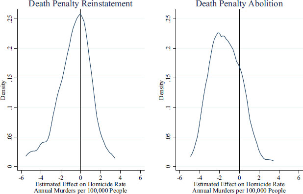
FIGURE 4-2 Distribution of regression-estimated effects across states.
SOURCE: Donohue and Wolfers (2005, p. 810, Figure 4). Used by permission.
penalty-intensity level) may have the same effect in each of these scenarios, it is also plausible that in the first setting the change in the sanction regime for murder would be perceived as small to potential murderers and in the second it would seem large. No research to date has explored whether the assumption that the treatment effect is insensitive to context created by other states is likely to hold, but violations of this assumption are known to lead to biased inferences (see, e.g., Rubin, 1986, p. 961). While accounting for social interactions is known to be difficult, Manski (in press) points to constructive ways of further addressing some of the problems that have been identified in the research to date.
The committee finds the failure of the panel studies we reviewed to address or overcome the primary challenges discussed above sufficient reason to view this research as noninformative with regard to the effect of the death penalty on homicides. The sanction regime is insufficiently specified and the measures of the intensity with which the death penalty is applied are flawed. No connection has been established between these measures and the perceived sanction risks of potential murderers. Neither
the fixed effects multiple regression models nor the proposed instruments are credible in overcoming challenges to identifying a causal link between the death penalty and homicide rates. The homogeneous response restriction that the effects are the same for all states and all time periods seems patently not credible.
Some researchers have argued that fixed effect models without instruments may provide valuable information, although not perfect information about the impact of death penalty on crime. One reason given is that they do not suffer from the defects that attend the use of manifestly invalid instrumental variables (see, for example, Donohue and Wolfers, 2009, and Kovandzic, Vieraitis, and Boots, 2009). This assessment of the informative value of the fixed effects models is dubious for several reasons. Most notably, these models do not address the data and modeling issues discussed throughout this chapter. The fixed effects models estimated in the literature do not specify the noncapital component of the sanction regime and setting aside the issue of how sanction risks are actually perceived, the measures of execution risk that are used do not appear to bear any resemblance to the true risk of execution. In addition, the key assumption that the death penalty sanction is independent of other unobserved factors that might influence homicide rates seems untenable. For these reasons, the fixed effects models are no more informative about the effect of the death penalty on homicide rates than other types of model.
Some studies play the useful role, either intentionally or not, of demonstrating the fragility of claims to have or not to have found deterrent effects (e.g., see Cohen-Cole et al., 2009; Donohue and Wolfers, 2005, 2009). However, even these studies suffer from the intrinsic shortcomings that severely limit what can be learned about the effect of the death penalty on homicide rates by using data on the death penalty as it has actually been administered in the United States in the past 35 years.
The challenges discussed here are formidable, and breakthroughs on several fronts would be necessary to overcome them. Only then might panel models, with or without instruments, be a fruitful methodology for studying the deterrent effects associated with the death penalty.
Alarcón, A.L., and Mitchell, P.M. (2011). Executing the will of the voters?: A roadmap to mend or end the California legislature’s multibillion-dollar death penalty debacle. Loyola of Los Angeles Law Review, 44(Special), S41-S224.
Angrist, J.D. (1990). Lifetime earnings and the Vietnam era draft lottery: Evidence from Social Security administrative records. American Economic Review, 80(3), 313-336.
Angrist, J.D., and Krueger, A.B. (1991). Does compulsory school attendance affect schooling and earnings? The Quarterly Journal of Economics, 106(4), 979-1,014.
Berk, R. (2005). New claims about executions and general deterrence: Déjà vu all over again? Journal of Empirical Legal Studies, 2(2), 303-330.
California Commission on the Fair Administration of Justice. (2008). Report and Recommendations on the Administration of the Death Penalty in California. Sacramento: Author.
Cohen-Cole, E., Durlauf, S., Fagan, J., and Nagin, D. (2009). Model uncertainty and the deterrent effect of capital punishment. American Law and Economics Review, 11(2), 335-369.
Cook, P.J. (2009). Potential savings from abolition of the death penalty in North Carolina. American Law and Economics Review, 11(2), 498-529.
Dezhbakhsh, H., and Shepherd, J.M. (2006). The deterrent effect of capital punishment: Evidence from a “judicial experiment.” Economic Inquiry, 44(3), 512-535.
Dezhbakhsh, H., Rubin, P.H., and Shepherd, J.M. (2003). Does capital punishment have a deterrent effect? New evidence from postmoratorium panel data. American Law and Economics Review, 5(2), 344-376.
Donohue, J.J., and Wolfers, J. (2005). Uses and abuses of empirical evidence in the death penalty debate. Stanford Law Review, 58(3), 791-845.
Donohue, J.J., and Wolfers, J. (2009). Estimating the impact of the death penalty on murder. American Law and Economics Review, 11(2), 249-309.
Durlauf, S., Navarro, S., and Rivers, D.A. (2010). Understanding aggregate crime regressions. Journal of Econometrics, 158(2), 306-317.
Fagan, J., Zimring, F.E., and Geller, A. (2006). Capital punishment and capital murder: Market share and the deterrent effects of the death penalty. Texas Law Review, 84(7), 1,803-1,867.
Frakes, M., and Harding, M.C. (2009). The deterrent effect of death penalty eligibility: Evidence from the adoption of child murder eligibility factors. American Law and Economics Review, 11(2), 451-497.
Katz, L., Levitt, S.D., and Shustorovich, E. (2003). Prison conditions, capital punishment, and deterrence. American Law and Economics Review, 5(2), 318-343.
Klick, J., and Tabarrok, A. (2005). Using terror alert levels to estimate the effect of police on crime. Journal of Law & Economics, 48(1), 267-279.
Kovandzic, T.V., Vieraitis, L.M., and Boots, D.P. (2009). Does the death penalty save lives? Criminology & Public Policy, 8(4), 803-843.
Lee, D., and McCrary, J. (2009). The Deterrent Effect of Prison: Dynamic Theory and Evidence. Unpublished paper. Industrial Relations Section, Department of Economics, Princeton University. Available: http://emlab.berkeley.edu/~jmccrary/lee_and_mccrary2009.pdf [December 2010].
Manski, C.F. (in press). Identification of treatment response with social interactions. Submitted to The Econometrics Journal. Available: http://onlinelibrary.wiley.com/doi/10.1111/j.1368-423X.2011.00368.x/abstract [December 2010].
Mocan, H.N., and Gittings, R.K. (2003). Getting off death row: Commuted sentences and the deterrent effect of capital punishment. Journal of Law & Economics, 46(2), 453-478.
Mocan, H.N., and Gittings, R.K. (2010). The impact of incentives on human behavior: Can we make it disappear? The case of the death penalty. In R.E.S. Di Tella and E. Schargrodsky (Eds.), The Economics of Crime: Lessons for and from Latin America (pp. 379-420). National Bureau of Economic Research conference report. Chicago: University of Chicago Press.
National Research Council. (1978). Deterrence and Incapacitation: Estimating the Effects ofCriminal Sanctions on Crime Rates. Panel on Research on Deterrent and Incapacitative Effects. A. Blumstein, J. Cohen, and D. Nagin (Eds.), Committee on Research on Law Enforcement and Criminal Justice. Assembly of Behavioral and Social Sciences. Washington, DC: National Academy Press.
Roman, J.K., Chalfin, A.J., and Knight, C.R. (2009). Reassessing the cost of the death penalty using quasi-experimental methods: Evidence from Maryland. American Law and Economics Review, 11(2), 530-574.
Rubin, D.B. (1986). Statistics and causal inference: Comment: Which ifs have causal answers. Journal of the American Statistical Association, 81(396), 961-962.
Shepherd, J.M. (2005). Deterrence versus brutalization: Capital punishment’s differing impacts among states. Michigan Law Review, 104(2), 203-255.
Snell, T.L. (2010). Capital Punishment, 2009—Statistical Tables. Report, U.S. Department of Justice (NCJ 231676). Available: http://www.ojp.usdoj.gov/index.cfm?ty=pbdetail&iid=2215. [December 2010].
Zimmerman, P.R. (2004). State executions, deterrence, and the incidence of murder. Journal of Applied Economics, 7(1), 163-193.


