
Appendix D
Long-Term Tide Gage Stability From Leveling Data
James Foster, University of Hawai’i at Manoa
Note: The committee commissioned the following discussion paper. Dr. Foster’s views, as expressed below, may not always reflect the views of the Committee on Sea Level Rise in California, Oregon, and Washington, or vice versa.
Abstract
Leveling observations from tide gage benchmark networks can be used to assess the long-term stability of the tide gage with respect to the benchmarks, to provide estimates on the degree to which short-term (e.g., decadal timescale) estimates of vertical motion can be inferred to represent longer term rates, and to provide a means for detecting and estimating possible steps in the sea-level record due to changes in tide gage instrumentation, monument instabilities or local ground motion. Leveling data from six California tide gages confirm that long-term vertical motions of the tide gages are small, typically less than 0.25 mm yr-1 with respect to the stable local coastline, and represent only a very minor portion of the relative sea-level change budget. Decadal timescale estimates of benchmark vertical motions mostly range between ± 0.5 mm yr-1 from their long-term values, indicating that decadal scale estimates of geodetic motion are generally a reasonable approximation to longer-term rates. The formal errors on the rate estimates however, based on an assumption of white noise, are over optimistically tight and should be scaled up by a factor of 2.33 to provide more realistic bounds. This analysis also suggests that the tide gage at Point Reyes may be experiencing recent subsidence, despite the long-term estimates indicating relative stability. Jumps were evident in the leveling data from all tide gages except Los Angeles: some are clearly due to changes in equipment, others are less clearly attributable to mechanical issues at the sites and may indicate corresponding steps remain uncorrected in the sea-level time series data.
INTRODUCTION
The observations recorded by tide gages are relative sea-level values, and are a linear combination of real changes in local sea level as well as any local vertical motions, due to either regional tectonics, local subsidence/uplift of the ground, and possibly offsets due to motions of the tide gage itself with respect to its mount. Routine leveling at tide gages has been performed for many decades, and provides a resource with which to explore the issues of local vertical land motions (Shinkle and Dokka, 2004) and tide gage stability over longer timescales than is possible with more modern geodetic techniques such as Global Navigation Satellite Systems (GNSS, such as GPS) measurements or satellite-based Interferometric Synthetic Aperture Radar (InSAR). With this data set it is possible to assess two key issues of importance to understanding long-term relative sea-level rise: (1) What proportion of the observed sea-level change is due to local vertical motions of the tide gage itself, or its immediate vicinity? (2) How representative are the vertical land motions estimated from GNSS/InSAR data over the last 5–15 years of multidecadal to century scale rates? Leveling data from 6 California tide gage networks (Figure D.1) were used to address these questions.
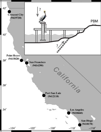
FIGURE D.1 Location of tide gages examined with inset showing schematic of a tide gage and benchmark leveling network illustrating fundamental ambiguity that may exist between motion of the tide gage instrument and local land motion.
Tide gages measure the height of the sea surface with respect to their own internal reference level. As the gages require relatively deep water to operate in, away from shore wave breaks and currents, they are often installed on manmade structures such as piers, built out from the coast. Although tide gage locations are chosen carefully in an effort to ensure long-term stability and a minimum of vertical motion, it is impossible to guarantee these qualities in a site. In order to maintain an accessible external reference mark from which the local sea-level datums can be assigned, to allow for tide gage equipment changes, and to confirm the stability of the gage, each tide gage is supported by a network of leveling benchmarks, with one of these designated as the primary benchmark. This is normally chosen to be both as close to the tide gage as possible, and installed in as stable a location as can be found (Hicks et al., 1987). As the local sea-level datums are defined with respect to this primary benchmark, each tide gage has a correction term that is applied to the raw ranges it observes to the sea-surface in order to map them to the vertical datum defined by the primary benchmark. Every time the gage is either changed, upgraded, or experiences some possible vertical offset—due, for example, to being hit by a harbor vehicle—a new correction term is calculated by performing leveling between the primary benchmark and the reference point on the new (or newly offset) tide gage. This term is applied to the data stream so that is it transparent to the end-user of the data, maintaining what is, in theory, a continuous record of sea level with respect to the primary benchmark, rather than the gage itself. Although these constants are recorded as they are recalculated and programmed into the tide gage data logger, they are not all archived digitally, and were not available for this study.
Current recommended operating procedures require a network of at least 10 benchmarks be established and monitored in support of tide gage sea-level observations (Woodworth, 2002). Historically, however, significantly fewer marks have been regularly observed—some of which may no longer exist due to construction (or other reasons) around the typically extremely changeable industrial environment of the harbors, where most tide gages are installed. Leveling of the west coast network is currently performed using 2nd Order Levels standards approximately annually, though historically it was often done much less frequently and to a lower standard. The leveling data are used to determine the general stability of each benchmark as well as the tide gage, and identify any tide gage offsets (any jump greater than 6 mm) necessitating a site correction factor adjustment. The long-term relative vertical velocity of the tide gage with respect to the primary benchmark is not applied as a correction to the sea-level time series.
DATA AND METHODS
The leveling data, corrected for atmospheric refraction, from all occupations of the tide gage benchmark networks for San Diego, Los Angeles, Port San Luis, San Francisco, Point Reyes, and Crescent City, were provided by the National Oceanographic and Atmospheric Administration’s (NOAA’s) Center for Operational Oceanographic Products and Services (CO-OPS). Each benchmark network data set con-
sisted of a spreadsheet listing the date of each leveling project and the height determined for each benchmark occupied during that project. The recorded heights themselves have little value for the purposes of this study, as they are determined with respect to some arbitrary starting height (typically a predefined value for the height of the primary benchmark) for each leveling run. The observations required for this study are changes in the height differences between benchmarks, so the first step was to determine the differential heights measured during each project with respect to the primary benchmark. A network solution was then performed to estimate and remove the mean differential height for each benchmark from the observations, generating a time series of observed changes in relative height for each benchmark in the network. Bad data points, due to incorrect readings or transcriptions of values, contaminate this initial analysis, and were identified and removed from the data set. These points are typically obvious as single observation outliers, displaced by several centimeters from the trend defined by the remainder of that benchmark’s data.
To interpret observed vertical motions and assess whether they are likely due to benchmark instability (Karcz et al., 1976) or rather to local land motions, the approximate spatial locations of the benchmarks are required. These locations were determined either by digitizing the survey benchmark sketches or, if available, extracted from the National Geodetic Survey (NGS) benchmark data sheet database. Some of the older, discontinued benchmarks have no recorded location and could not contribute to this aspect of the analysis. In most cases, the digitized locations of the benchmarks are estimated to be accurate to 40 m or better, while those determined by the NGS using GPS or other methods are considerably more accurate. This accuracy is sufficient to allow us to examine and interpret spatial patterns of vertical motions. Benchmarks interpreted as being unstable are identified from their time series, either objectively by virtue of very high variance about their mean trend (typically greater than 10 mm2, in contrast to most benchmarks which have variances typically less than 2 mm2), or more subjectively due to having high apparent relative vertical velocities, uncorrelated with their neighboring marks, by comparison with the rest of the network. In most cases, those benchmarks identified as unstable have been given a stability rating of C or D by the NGS, indicating unknown or doubtful long-term stability. However, in some cases even benchmarks with the highest A rating were found to have velocities and/or variances at odds with the neighboring marks.
Both the formal NGS/CO-OPS datum definition and, at this stage in the processing, this analysis, define the primary benchmark as a fixed reference. There is clearly a danger, however, that the primary benchmark itself might experience vertical motions, due either to local benchmark instability or real land motions. In order to assess and account for this, a subset of the benchmarks in the network that show no sign of either monument instability or anomalous rates of motion was used to define a combined vertical reference datum for the network, which should provide a more robust datum. The choice of benchmarks is somewhat subjective, and is unable to correct for vertical deformation occurring on spatial scales greater than the width of the network. It turns out, however, that the specific choice of reference benchmarks has only a small impact on the final estimates of rates of vertical motion for the tide gage and primary benchmark.
The rates of vertical motion were estimated using a robust linear fit that uses an iterative reweighting scheme to reduce the impact of outlier observations on the final estimation of slope. To assess the degree to which estimates of vertical motions based on decadal scale windows of data can be trusted as reasonable approximations to the longer-term trends, a moving window was applied to the data set, and vertical rates for each window were estimated. A minimum of 5 observations and at least a 10-year time span were required for each window location in order to generate an estimate for any given period in order to prevent the results being merely a reflection of the measurement errors and/or sparse data.
RESULTS
San Diego
Three benchmarks—9, N 57, and RIVET— showed anomalous vertical motions and were excluded from the spatial analysis. Benchmarks RIVET and N 75 were given a D stability code by the National Geodetic Survey, indicating they might be expected
to be unstable. Benchmark 9, on the other hand, has an A rating, indicating highest level of confidence in the benchmark stability. It is, however, located in the middle of downtown San Diego, and it is possible that this location has over the decades experienced significant vertical motion due to construction and settling, unrelated to broader underlying tectonic trends. For the remaining network (Figure D.2), vertical motions suggest a gentle northwest to southeast trend, with the majority of benchmarks nearest to the tide gage location in close agreement. Defining a network vertical reference using these sites implies a vertical motion for the primary benchmark of -0.03 mm yr-1, and for the tide gage reference marks of +0.07 mm yr-1. Estimating the apparent decadal scale vertical velocities by calculating rates for each 10 consecutive measurements shows that these rates range from -0.4 mm yr-1 to nearly 1 mm yr-1, though mostly clustered between ± 0.2 mm yr-1. The exceptional rates in the 1980s are possibly due to a small, unmodeled residual step in the tide gage leveling time series, either at the tide gage itself, or possibly at the primary benchmark, as the other benchmark time series also show excursions at this time. With less consistent and rigorous field operational procedures, data prior to 1970 are noisier, and this is reflected in the increased range and errors for the velocity estimates for this period.
Los Angeles
Los Angeles is recognized as having complex temporal and spatial variations in vertical deformation (Brooks et al., 2007), and this complexity is evident in the range of vertical motions calculated for the tide gage leveling network and their spatial pattern (Figure D.3; for which the limited and inconsistent 4 measurements for a STAFF STOP tide gage mark were ignored). Although it appears that a large portion of the pier on which the tide gage is installed is experiencing significant subsidence relative to the coast, the end nearest the tide gage and primary benchmark sees less of this. The choice of benchmarks for the network vertical reference is particularly difficult for this location, as there is no obvious subset of benchmarks demonstrating broadly similar motion that might be interpreted as “stable.” However, excluding benchmarks with the most extreme motions results in a reference
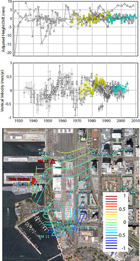
FIGURE D.2 (Top) Time series of vertical displacements for San Diego (9410170) tide gage leveling network. All benchmarks are shown in gray except tide gage marks RM OF ETG (yellow) and AQUATRAK (cyan). (Middle) Time series of apparent vertical velocities based on at least 5 consecutive observations covering at least 10 years (approximately decadal). All benchmarks are shown in gray except tide gage marks RM OF ETG (yellow) and AQUATRAK (cyan). (Bottom) Contours of best-fit linear vertical deformation rates for San Diego benchmarks with respect to network vertical reference frame. Contours every 0.1 mm yr-1.
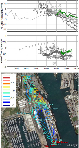
FIGURE D.3 (Top) Time series of vertical displacements for Los Angeles (9410660) tide gage leveling network. All benchmarks shown in gray except tide gage mark AQUATRAK (green). (Middle) Time series of apparent decadal-scale vertical velocities. All benchmarks shown in gray except tide gage mark AQUATRAK (green). (Bottom) Contours of best-fit linear vertical deformation rates for Los Angeles benchmarks with respect to network vertical reference frame. Contours every 0.1 mm yr-1.
frame in which the primary benchmark is experiencing 0.14 ± 0.14 mm yr-1 uplift, and the tide gage subsiding at 0.17 ± 0.12 mm yr-1. The large errors probably reflect the strong quasi-seasonal signals recognized in Los Angeles (Bawden et al., 2001) that will be strongly aliased into the roughly annual leveling campaigns. The vertical velocity time series suggests relatively large variations in apparent velocities on the decadal scale, with a strong perturbation in the 1990s due largely to a leveling run that recorded unusual, but not obviously incorrect, values.
Port San Luis
The benchmark network at Port San Luis appears particularly stable, with the exception of two benchmarks (B and H 828), which were removed from the analysis. The network vertical reference implies a small uplift of 0.08 ± 0.05 mm yr-1 for the primary benchmark, and slight subsidence of 0.05 ± 0.05 mm yr-1 for the tide gage, which for this location is located at the end of a long pier (Figure D.4). Notably, there is a distinct downward step in the leveling time series for both tide gage marks in 1996 with a mean value of -5.25 ± 0.59 mm. It is not clear whether this step is a result of equipment change or some other source; however, it should be noted that when corrected, the sign of the tide gage motion changes, with slight uplift indicated (0.29 ± 0.05 mm yr-1). All plots in Figure D.4 show the data after these steps have been estimated and removed from the time series. If left in, this step dominates the analysis of the decadal-scale velocity estimate stability. If removed, however, the short-term velocities indicate that all (stable) benchmarks are well described over their lifetime by a consistent vertical velocity.
San Francisco
San Francisco has a very long record of benchmark leveling, with the earliest measurements dating from the mid 1920s. Several of the benchmarks show significant excursions over that time period (Figure D.5), yet the long-term pattern is of relative consistency. Steps were estimates and removed from benchmarks 173 (in 1943) and 175 (in 1980). Benchmarks M and 175 were considered outlier time series and not included in the spatial analysis. The network vertical reference
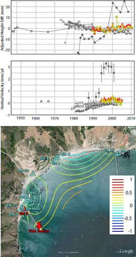
FIGURE D.4 (Top) Time series of vertical displacements for Port San Luis (9412110) tide gage leveling network. All benchmarks shown in gray except tide gage marks AQUAREF (yellow) and AQUATRAK (red). Steps in the tide gage time series have been removed. Unstable benchmark BM B clearly visible as outlier time series. (Middle) Time series of apparent decadal-scale vertical velocities. All benchmarks shown in gray except tide gage marks AQUAREF (yellow) and AQUATRAK (red). (Bottom) Contours of best-fit linear vertical deformation rates for Port San Luis benchmarks with respect to network vertical reference frame. Contours every 0.1 mm yr-1.
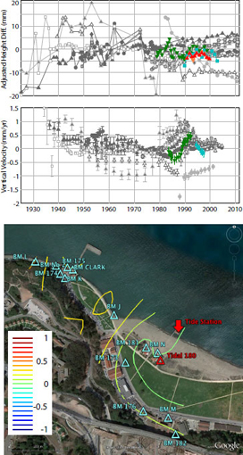
FIGURE D.5 (Top) Time series of vertical displacements for San Francisco (9414290) tide gage leveling network. All benchmarks shown in gray except tide gage marks AQUATRAK REF (red), AQUATRAK (cyan), RM OF ETG (green) and STAFF STOP (orange). (Middle) Time series of apparent decadal-scale vertical velocities. All benchmarks shown in gray except tide gage marks AQUATRAK (cyan) and RM OF ETG (green) (AQUATRAK REF and STAFF STOP did not have long enough time series to generate decadal velocity estimates). (Bottom) Contours of best-fit linear vertical deformation rates for San Francisco benchmarks with respect to network vertical reference frame. Contours every 0.1 mm yr-1.
analysis suggests that in late 1989—around the time of the Loma Prieta earthquake—the primary benchmark moved with respect to the rest of the network. Correcting the data for this motion does not entirely remove the apparent upward motions of several benchmarks at this time, or shortly afterward, suggesting that the monuments or the local ground around them moved either during the shaking of the earthquake itself or during a period of post-seismic adjustment. Despite this, the rate of motion calculated for the primary benchmark is small (0.05 ± 0.07 mm yr-1) and the mean tide gage motion is negligible (0.01 ± 0.07 mm yr-1). As there is little spatial coherence in the vertical velocities, with adjacent benchmarks often exhibiting opposite senses of motion, the contour map results in only small amplitude variability in vertical motion rates. The decadal-scale vertical velocities are strongly affected by the 1989 events, but nonetheless generally indicate that estimates of long-term vertical motions based on any 10-year period would be accurate to better than 0.5 mm yr-1.
Point Reyes
Although the time series from Point Reyes is relatively short, with the first regular observations starting in 1973 (an initial leveling run in 1930 was too removed from the rest of the data set to contribute usefully to the analysis), it shows relatively complex behavior (Figure D.6). The AQUAREF mark, observed between 1990 and 1999, shows strong linear downward motion, at odds with the other tide gage mark, AQUATRAK, and were ignored during the spatial analysis, as were outlier records from benchmarks 1 FMK and 11. The benchmark leveling observations, which were otherwise largely stable prior to ~2001, show strong heterogeneous motions after this point, with many sites uplifted for several years before subsiding back to their long-term baselines. The recent AQUATRAK record, however, shows continued subsidence. The contour plot highlights an area experiencing significant uplift to the southeast of the tide gage, with all other benchmarks appearing relatively stable over the full time window of the observations. This uplift may be related to motion on a mapped fault segment (Clark and Brabb, 1997) near the eastern edge of the network. Although there is no evidence to suggest this fault is affecting the
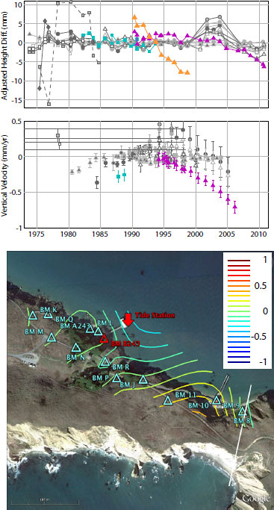
FIGURE D.6 (Top) Time series of vertical displacements for Point Reyes (9415020) tide gage leveling network. All benchmarks shown in gray except tide gage marks AQUAREF (orange), AQUATRAK (magenta) and RM OF ETG (blue). ( Middle) Time series of apparent decadal-scale vertical velocities. All benchmarks shown in gray except tide gage marks AQUAREF ( orange), AQUATRAK (magenta) and RM OF ETG (blue). ( Bottom) Contours of best-fit linear vertical deformation rates for Point Reyes benchmarks with respect to network vertical reference frame. Contours every 0.1 mm yr-1. White line indicates mapped fault trace.
tide gage itself, it emphasizes the tectonic complexity of many locations along the California coast. The velocity stability analysis highlights the AQUAREF outlier velocities, suggesting that these observations are most likely indicating monument instability. The other benchmarks have decadal velocity estimates consistent to ± 0.5 mm yr-1, until the impact of the events of 2001–2011, which indicate some possibly transient deformation event affecting a subset of the benchmark network. Interestingly, the vertical velocity rate estimates for the AQUATRAK suggest continued, or even accelerating subsidence, with the most recent decadal rate approaching -1 mm yr-1.
Crescent City
Long-term relative height residuals are generally small, though several benchmarks show unusually large motions compared to the rest of the network, presumably due to benchmark instability (Figure D.7). The pattern of the contours suggest that the benchmarks nearest the main downtown area are being uplifted slightly relative to the benchmarks around the port. It is perhaps more likely that the port area is subsiding; however, the relative rates are small. The velocity analysis highlights one of the more unstable benchmarks (NO 24), which was excluded from the contouring solution, along with outliers PASS and 18. It also, however, highlights a change in behavior of the RM OF ETG tide gage mark in the late 1980s. Following a relatively small possible step in the time series sometime between September 1986 and September 1987, there is a strong change in decadal vertical velocity. A large step in November 1988 indicates a change in equipment. However, the apparent motion continues past this date, perhaps indicating a problem with the tide gage monument, as the AQUATRAK mark, observed from 1989, does not show the same motion. For the other marks, decadal velocity estimates are generally within ± 0.4 mm yr-1, indicating long-term rates can be reasonably reliably inferred from relatively short-term observation records.
DISCUSSION
The locations of tide gages are chosen to be stable, and so it is unsurprising—though reassuring—that in
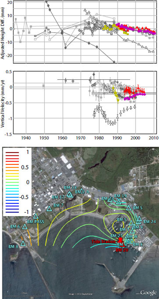
FIGURE D.7 (Top) Time series of vertical displacements for Crescent City (9419750) tide gage leveling network. All benchmarks shown in gray except tide gage marks AQUAREF (magenta), AQUATRAK (red) and RM OF ETG (yellow). (Middle) Time series of apparent decadal-scale vertical velocities. All benchmarks shown in gray except tide gage marks AQUAREF (magenta), AQUATRAK (red) and RM OF ETG (yellow). (Bottom) Contours of best-fit linear vertical deformation rates for Crescent City benchmarks with respect to network vertical reference frame. Contours every 0.1 mm yr-1.
general they show only small vertical motions with respect to their benchmark leveling networks (Table D.1). Some of the motions approach 0.25 mm yr-1, however, which is large enough that they should be accounted for when assessing the long-term rates of relative sea-level rise. The data indicate that, although the long-term vertical motion rates are small, there are significant spatial and temporal variations in these rates within several of the networks. Although several instances of apparent monument instability are evident, in most cases these motions appear to reflect real local ground motions. Some of these spatial patterns appear to be consistent over the time window of leveling observations, but others show changes in behavior over time. In particular, the San Francisco tide gage network appears to have been significantly affected by the Loma Prieta earthquake, while Point Reyes appears to have experienced a longer period event, whose impact might still be influencing the tide gage.
Another issue of concern is the impact of tide gage monument instability on estimates of relative sea-level change. Standard procedures for tide gage operations and maintenance of the local vertical reference datum include programming the tide gage data logger with a correction constant that takes into account changes in the instrument height during equipment changes or other events. In particular, any change of more than 6 mm is assumed to reflect instrument monument instability and should be accounted for by a change in the correction constant. Unfortunately, although the values of these constants and when they were changed have been recorded and archived, they are mostly in
TABLE D.1 Long-Term Vertical Motion Estimates for Primary Benchmarks and Tide Gage Reference
| Tide Gage Location | Benchmark | Vertical Velocity (mm yr-1) | Velocity Error (mm yr-1)a | Data Range |
| San Diego (9410170) | 12 (primary benchmark) AQUATRAK RM of ETG Mean |
-0.03 +0.06 +0.08 -.0.07 |
0.02/0.05 0.05/0.12 0.05/0.12 0.02/0.05 |
1917–2011 1990–2011 1966–1994 |
| Los Angeles (9410660) | 8-14 FT ABOVE MLLW (primary benchmark) AQUATRAK STAFF STOP Mean |
+0.14 -0.17 +126 -0.17 |
0.14/0.33 0.14/0.33 144/335 0.14/0.33 |
1920–2011 1990–2011 1980–1984 |
| Port San Luisb (9412110) | 6 (primary benchmark) AQUAREF AQUATRAK Mean |
+0.08) (-0.10) +0.24) (-0.03) +0.32) (-0.05)+0.29) |
0.05/0.12 (0.11)0.09/0.21 (0.08) 0.07/0.16 (0.05) 0.05/0.12 |
1933–2011 1989–2011 1989–2011 |
| San Francisco (9414290) | 180 (primary benchmark) AQUATRAK REF AQUATRAK RM of ETG STAFF STOP Mean |
-0.05 -0.06 -0.06 -0.01 +0.16 -0.01 |
0.07/0.16 0.12/0.28 0.12/0.28 0.10/0.23 0.17/0.40 0.07/0.16 |
1925–2011 1990–2000 1989–2003 1978–1999 1991–1999 |
| Point Reyes (9415020) | B243 (primary benchmark) AQUAREF AQUATRAK RM of ETG Mean |
+0.03 -1.78 -0.28 -0.22 -0.22 |
0.02/0.05 0.11/0.26 0.05/0.12 0.07/0.16 0.07/0.16 |
1930–2011 1990–1999 1990–2011 1982–1994 |
| Crescent City (9419750) | TIDAL 20 1959 RESET (primary benchmark) AQUAREF AQUATRAK RM of ETG Mean |
+0.05 -0.24 -0.11 -0.23 -0.20 |
0.03/0.07 0.04/0.09 0.05/0.12 0.09/0.21 0.06/0.14 |
1933–2011 1989–2011 1989–2011 1982–1996 |
a Two error estimates are listed: the formal error and the formal error multiplied by the empirically determined 2.33 scale factor.
b Values for Port San Luis in parentheses are calculated before a ~6.5 mm step in 1996 is removed from the time series.
analog form and were not available to this study. Without them it becomes impossible to say with complete confidence whether any particular step detected in the leveling data for a tide gage has been accurately removed a priori from the sea-level time series by adjustment of the on-site correction value. Each of San Diego, Point Reyes and Crescent City tide gages have significant steps in the leveling (Table D.2) that appear to match detectable steps in the sea-level record (Larry Breaker, personal communication). The smaller of these (e.g., 11.2 mm at San Diego) would have only a minor impact on long-term sea-level change estimates; however the larger ones, if entirely uncorrected, could contribute significantly to apparent rates of change. It is unclear whether it is possible to retroactively determine whether these steps have been entirely, partly, or not corrected. This problem increases the ambiguity of whether a leveling step indicates a recognized change or step in the tide gage instrumentation, a problem with the mounting of the tide gage instrument, or motion of the entire pier, due to either settling or, possibly, local ground motion.
The analysis of the stability of decadal-scale velocity estimates suggests that, for most tide gages and benchmark networks, although there is significant variation over the full time window, the limited range suggests it is largely reasonable to extrapolate vertical rates based on a limited time window of observations. Figure D.8 shows the rate differences between the decadal-scale rate estimates and the final “correct” long-term estimate. These results confirm that the decadal-scale rate estimates are tightly clustered around their long-term values with 2σ = 0.48 mm yr-1. The same data can be mapped into differences expressed as multiples of the formal errors determined for the decadal-scale rate estimates (Figure D.8 right). Presented this way, the 2σ limits indicate that the formal errors for the decadal rate estimates are significantly too optimistic, with the 2σ value being 4.66. Interestingly this 2.33 multiple of the formal error is close to the 2.5 empirical scale factor often adopted in GPS geodesy to take account of red noise in the time series produced by quasi-seasonal and other long-term signals. Detailed analyses of the noise character of GPS coordinate time series (Mao et al., 1999; Williams et al., 2004) find that the errors are typically well described by a power-law function. The results presented here suggest that the same power-law functions describing noise in decadal-scale GPS vertical time series may also be applicable to multi-decadal leveling measurements.
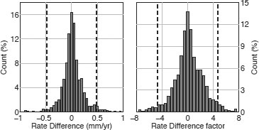
FIGURE D.8 Histograms of differences between decadal-scale estimates of vertical motion rates and the long-term rate determined from the full time series. (Left) Rate differences observed in mm yr-1. (Right) Rate differences expressed as multiples of the formal error determined for the decadal velocity ft.
TABLE D.2 Steps Detected in Tide Gage Leveling Marks
| Location | Step Size (mm) | Step Date |
| San Diego | +11.2 | Early 1974 |
| Port San Luis | -6.5 | Between late 1995 and late 1996 |
| San Francisco | +15.0 | May 9, 1979 |
| San Francisco | -5.0 | Between November 17, 1983, and May 31, 1984 |
| Point Reyes | +42.3 | 1994 |
| Crescent City | +84.5 | Between November 2 and 9, 1988 |
| Crescent City | +3.0 | Between September 1986 and September 1987 |
REFERENCES
Bawden, G.W., W.R. Thatcher, R.S. Stein, K.W. Hudnut, and G. Peltzer, 2001, Tectonic contraction across Los Angeles after removal of groundwater pumping effects, Nature, 412, 812-815.
Brooks, B.A., M.A. Merrifield, J. Foster, C.L. Werner, F. Gomez, M. Bevis, and S. Gill, 2007, Space geodetic determination of spatial variability in relative sea level change, Los Angeles Basin, Geophysical Research Letters, 34, L01611, doi:10.1029/2006GL028171.
Clark, J.C., and E.E. Brabb, 1997, Geology of Point Reyes National Seashore and Vicinity, California: A Digital Database, U.S. Geological Survey Open File Report 97-456, available at <http://pubs.usgs.gov/of/1997/of97-456/>.
Hicks, S.D., P.C. Morris, H.A. Lippincott, and M.C. O’Hargan, 1987, User’s Guide for the Installation of Bench Marks and Leveling Requirements for Water Level Stations, NOAA National Ocean Service, Rockville, MD, 73 pp.
Karcz, I., J. Morreale, and F. Porebski, 1976, Assessment of benchmark credibility in the study of recent vertical crustal movements, Tectonophysics, 33, T1-T6.
Mao, A., C.G.A. Harrison, and T.H. Dixon, 1999, Noise in GPS coordinate time series, Journal of Geophysical Research, 104, 2797-2816.
Shinkle, K.D., and R.K. Dokka, 2004, Rates of Vertical Displacement at Benchmarks in the Lower Mississippi Valley and the Northern Gulf Coast, NOAA Technical Report NOS/NGS 50, 135 pp.
Williams, S.D.P., Y. Bock, P. Fang, P. Jamason, R.M. Nikolaidis, L. Prawirodirdjo, M. Miller, and D.J. Johnson, 2004, Error analysis of continuous GPS position time series, Journal of Geophysical Research, 109, B03412, doi:10.1029/2003JB002741.
Woodworth, P.L., 2002, Manual on Sea Level Measurement and Interpretation, Volume III - Reappraisals and Recommendations as of the Year 2000, Intergovernmental Oceanographic Commission, Manuals and Guides, 14, 49 pp.
ACKNOWLEDGMENTS
Thanks to Todd Ehret of NOAA CO-OPS for providing the leveling data and Clyde Kakazu, Marti Ikehara, and Stephen Gill for valuable discussion about the NGS/CO-OPS leveling procedures and data handling and archiving.
GLOSSARY
|
AQUAREF/AQUATRAK REF |
Physical point on tide gage used for leveling |
|
AQUATRAK |
Physical point on tide gage used for leveling |
|
Primary Bench Mark (PBM) |
Benchmark which defines the local vertical datum |
|
RM OF ETG |
Physical point on tide gage used for leveling (reference mark of electric tape gage) |
| STAFF STOP | Physical point on tide gage used for leveling |
This page intentionally left blank.


