Below are the first 10 and last 10 pages of uncorrected machine-read text (when available) of this chapter, followed by the top 30 algorithmically extracted key phrases from the chapter as a whole.
Intended to provide our own search engines and external engines with highly rich, chapter-representative searchable text on the opening pages of each chapter. Because it is UNCORRECTED material, please consider the following text as a useful but insufficient proxy for the authoritative book pages.

Do not use for reproduction, copying, pasting, or reading; exclusively for search engines.

OCR for page 33
3 Contributions to Global Sea-Level Rise S ea-level rise is governed by processes that alter the Fourth Assessment Report, then evaluates more recent volume of water in the global ocean--primarily results. thermal expansion of sea water and transfers of water from terrestrial reservoirs, such as land ice and THERMAL EXPANSION groundwater, to the ocean. The Intergovernmental Panel on Climate Change (IPCC) Fourth Assessment Sea level is affected by changes in the density of sea Report found that thermal expansion accounted for water, induced by temperature changes ( thermosteric) about one-quarter of the observed sea-level rise for or by salinity changes (halosteric). Freshening of the 1961­2003, melting of land ice accounted for less than water column (halosteric expansion) has been esti- half, and changes in land water storage accounted for mated to account for about 10 percent of the global less than 10 percent (Bindoff et al., 2007). For the last average steric sea-level rise during recent decades (e.g., 10 years of that period (1993­2003), the IPCC esti- Antonov et al., 2002; Munk, 2003; Ishii et al., 2006). mated that thermal expansion and land ice melt each However, only about 1 percent of the halosteric ex- contributed about half to the total sea-level rise. The pansion contributes to the global sea-level-rise budget improved agreement between estimates of the indi because ocean mixing increases the salinity and thus vidual contributions and the total sea-level rise for the decreases the volume of the added freshwater (Bindoff later time period was attributed to the availability of et al., 2007). Consequently, only the thermosteric com- satellite altimetry data and other global ocean data sets ponent is discussed below. and to better knowledge of the processes causing sea- When the ocean warms, seawater becomes less level rise. Subsequent work has corrected instrument dense and expands, raising sea level. Because warm biases, reducing estimates of the thermal expansion water expands more than cold water with the same contribution to sea-level rise, and recorded increased amount of heating, and seawater at higher pressure rates of land ice loss. In the most recent estimate, for expands more than seawater at lower pressure, global 1993­2008, the contribution from land ice increased to sea-level change depends on the distribution of ocean 68 percent, the contribution from thermal expansion temperature change throughout the ocean, from top decreased to 35 percent, and land water storage con- to bottom. Thermosteric sea-level change is calcu- tributed -3 percent (sea-level fall; Church et al., 2011). lated from temperature and pressure measurements This chapter evaluates the contributions of thermal made from a wide variety of instruments that descend expansion, glaciers, ice sheets, and other terrestrial through the water column, are towed from ships, or are sources of water to global sea-level rise. Each section attached to moored and drifting buoys and profiling begins with a summary of findings from the IPCC floats (see Johnson et al., 2006). 33

OCR for page 33
34 SEA-LEVEL RISE FOR THE COASTS OF CALIFORNIA, OREGON, AND WASHINGTON Estimates from the IPCC Fourth Assessment Report Recent Estimates The IPCC Fourth Assessment Report found that At about the time the IPCC Fourth Assessment warming in all three of the major ocean basins has oc- Report was published, systematic efforts began to be curred over the past few decades (Bindoff et al., 2007). made to correct for biases in the expendable bathy Further, thermal expansion of the global ocean (ther- thermo graph (XBT) and mechanical bathythermo- mosteric sea-level rise) exhibits significant decadal and graph (MBT) data, which constitute the majority of interannual variations. Thermosteric sea-level rise was ocean temperature observations prior to 2002, and in estimated to account for approximately one-quarter of Argo data (Box 3.1). These biases affected the tem- the observed rate of global sea-level rise from 1961 to perature inferred from measurements and thus the 2003, contributing 0.32 ± 0.12 mm yr-1 down to 700 m calculated rate of thermosteric sea-level rise. Thermo- depth and 0.42 ± 0.12 mm yr-1 down to 3000 m depth. steric sea-level trends have recently been reanalyzed For the last 10 years of that period (1993­2003), the using bias-corrected temperature data, and the record contribution of thermal expansion was estimated to has been extended by new observations. In addition, a have increased to 1.5 ± 0.5 mm yr-1 above 700 m and few new estimates of the thermosteric fraction of sea 1.6 ± 0.5 mm yr-1 above 3,000 m, about half of the level have been made using data assimilation products observed rate of global sea-level rise. and satellite data. BOX 3.1 Bathythermograph and Argo Measurements Bathythermographs are dropped from ships and transmit temperature via a thin wire as they sink through the water column. Mechanical bathyther- mographs (MBTs) record temperature at 5 m depth intervals down to approximately 285 m. Thus, they are useful only for studying the thermal structure of the upper ocean. The successor expendable bathythermographs (XBTs) can provide temperature profiles to depths of approximately 760 m (standard instruments) or 1,830 m (special instruments). Data from MBTs and/or XBTs are available since 1948. Ocean profiling floats are deployed under the multi-national Argo program and by individual countries. Argo profiling floats began measuring the temperature and salinity of the upper 1,000­2,000 m of the ocean in 2000. The Argo array currently comprises more than 3,000 ocean profiling floats distributed around the world (see Figure). Data from these floats are collected via satellite. 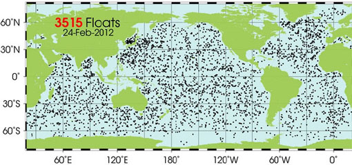FIGURE Distribution of Argo profiling drifters on February 24, 2012. These floats measure salinity and temperature over the upper 1,000­2,000 m of the ocean. SOURCE: These data were collected and made freely available by the International Argo Program and the national programs that contribute to it (, ).

OCR for page 33
CONTRIBUTIONS TO GLOBAL SEA-LEVEL RISE 35 In Situ Data Recent observational estimates of thermosteric sea- level rise have all been corrected for XBT and MBT A time-varying warm bias (systematically warmer depth bias (Table 3.1). The new estimates are based on temperature than the true value) has been found in updates of the Ishii and Kimoto (2009) data set (e.g., the global XBT data, and a cold bias (systematically Ishii, personal communication; Kuo and Shum, per- colder temperature than the true value) has been found sonal communication), which corrects for depth bias, in a small fraction of Argo float data (e.g., Gouretski or the Ingleby and Huddleston (2007) data set (e.g., and Koltermann, 2007; Wijffels et al., 2008; Ishii and Domingues et al., 2008), which corrects for both XBT Kimoto, 2009; Willis et al., 2009). XBT and MBT fall-rate bias and undersampling bias. Their estimates temperature observations are subject to instrument of the long-term thermosteric trend (beginning 1951­ bias, such as depth bias. The depth of each tempera- 1961) in the upper 700 m of the ocean range from ture observation is calculated using a fall-rate equation 0.29 ± 0.06 mm yr-1 to 0.52 ± 0.08 mm yr-1 (Table 3.1). and the time elapsed since the XBT entered the water. The latter, by Domingues et al. (2008), is higher than Inaccuracies in the fall rate affect the apparent depth at the rates estimated by IPCC (2007) for the same period which the temperature profile is taken, which in turn and by other investigators for similar periods. Estimates causes a temperature bias that varies with depth. The of the thermosteric trend in the upper ocean since 1993 MBT depth bias may have resulted from a delayed range from 0.71 ± 0.31 mm yr-1 to 1.23 ± 0.30 mm yr-1 response by the diaphragm used to sense pressure and (Table 3.1). These rates are generally lower than those thus infer depth (Gouretski and Koltermann, 2007). estimated by the IPCC (2007) for 1993 to 2003. The Argo biases were associated with a particular set Observations for the deep ocean are sparse, so of instruments deployed mainly in the Atlantic Ocean thermal expansion estimates for the full ocean depth (Willis et al., 2009). The sensors on these instruments are more uncertain than those for the upper ocean. use pressure measurements to infer depth, but a flaw The only recent estimates of the rate of thermosteric caused temperature and salinity values to be associated sea-level rise for the full ocean depth are by Domingues with incorrect pressure values, biasing the data. et al. (2008) and Church et al. (2011), who used a Correcting for XBT depth bias reduced the mag- thermal expansion value of 0.2 ± 0.1 mm yr-1 and nitude of the interdecadal variability previously seen 0.17 mm yr-1, respectively, for the deep ocean. This in the thermosteric sea-level signal during the 1970s deep-ocean value is comparable to a recent estimate of (Domingues et al., 2008). An apparent sharp rise in ~0.15 ± 0.08 mm yr-1 based on abyssal (below 4,000 m) thermosteric sea level during the 1970s was greatly and deep ocean (1,000­4,000 m) observations south of decreased in the corrected data of Levitus et al. (2009), the SubAntarctic Front taken in the 1990s and 2000s and essentially disappeared in the corrected data of Ishii (Purkey and Johnson, 2010). Kouketsu et al. (2011) es- and Kimoto (2009; compare the dotted and solid red and timated thermosteric sea-level change of ~0.11 mm yr-1 blue lines in Figure 3.1, top). Correcting for depth bias for the ocean below 3,000 m from the 1990s and to the also changed the estimated rate of global thermosteric 2000s based on observed data, and 0.12 mm yr-1 based sea-level rise. For example, Ishii et al.'s (2006) original on an ocean model data assimilation product. The estimate of thermosteric sea-level rise for the upper IPCC (2007) assessment, based on work by Antonov 700 m was 0.26 ± 0.06 mm yr-1 from 1951 to 2005. et al. (2005), was 0.1 mm yr-1 from 700 m to 3,000 m After correcting XBT and MBT temperatures for depth (Bindoff et al., 2007). Given the scarcity of data, how- bias and using an improved temperature climatology, ever, it is difficult to assess the uncertainty in deep Ishii and Kimoto (2009) found a slightly higher rate of ocean warming. 0.29 ± 0.06 mm yr-1 for the same time period (Table 3.1). Domingues et al. (2008) estimated that thermosteric Discarding biased Argo profiles removed an ap- sea-level rise for the full ocean depth increased from parent cooling trend from 2003 to 2006 (Willis et al., 0.72 ± 0.13 mm yr-1 for 1961­2003 to 1.0 ± 0.4 mm yr-1 2009). The linear trend from January 2005 to September for 1993­2003 (Table 3.1). The Church et al. (2011) 2011 in the newly analyzed data is 0.48 ± 0.15 mm yr-1 estimates for 1993­2008 are 0.88 ± 0.33 mm yr-1. For (Figure 3.2, Table 3.1). comparison, the committee calculated thermosteric sea-

OCR for page 33
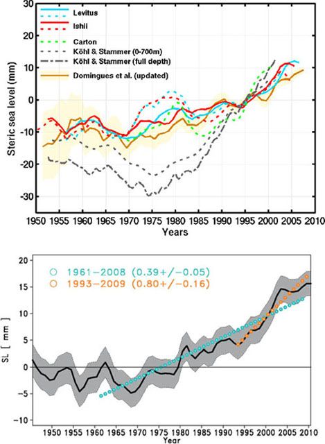
36 SEA-LEVEL RISE FOR THE COASTS OF CALIFORNIA, OREGON, AND WASHINGTON FIGURE 3.1(Top) Estimates of global mean thermosteric sea level for the past six decades. The dotted blue and red lines are the IPCC (2007) estimates for the upper 700 m. The solid blue and red lines are the equivalent curves after correction for XBT biases. Also shown are a bias-corrected estimate for the upper 700 m by Domingues et al. (2008; brown line with 1 standard deviation shaded) and an uncorrected estimate down to 1,000 m from the Simple Ocean Data Assimilation model by Carton et al. (2005; green dotted line). Estimates from the ocean data assimilation model of Kohl and Stammer (2008) to 700 m (gray dotted line) and full depth (gray dash-dotted line) also are shown. SOURCE: Church et al. (2010). (Bottom) New estimate of global mean thermosteric sea-level rise for the upper 700 m using an updated version of bias-corrected data from Ishii and Kimoto (2009). The orange and blue symbols and values are linear thermosteric sea-level trends for different time periods. The gray shading represents 1 standard deviation. SOURCE: Ishii and Kimoto (2009).

OCR for page 33
CONTRIBUTIONS TO GLOBAL SEA-LEVEL RISE 37 TABLE 3.1 Recent Estimates of Global Mean Thermosteric Sea-Level Rise Thermosteric Sea-Level Rise Source Period Depth Range (m) Instrument Bias Corrections (mm yr-1) IPCC (2007) 1961­2003 0­700 None 0.32 ± 0.12 0­3,000 0.42 ± 0.12 Domingues et al. (2008) 1961­2003 0­700 XBT fall-rate bias 0.52 ± 0.08 Full depth 0.72 ± 0.13 Ishii and Kimoto (2009) 1951­2005 0­700 XBT and MBT depth bias 0.29 ± 0.06 Kuo and Shum (personal communication, 2011)a 1955­2009 0­700 XBT and MBT depth bias 0.33 ± 0.01 Ishii (personal communication, 2011)b 1961­2008 0­700 XBT and MBT depth bias 0.39 ± 0.05 IPCC (2007) 1993­2003 0­700 None 1.5 ± 0.5 0­3,000 1.6 ± 0.5 Domingues et al. (2008) 1993­2003 0­700 XBT fall-rate bias 0.79 ± 0.39 Full depth 1.0 ± 0.40 Ishii and Kimoto (2009) 1993­2005 0­700 XBT and MBT depth bias 1.23 ± 0.30 Ishii (personal communication, 2011)b 1993­2009 0­700 XBT and MBT depth bias 0.80 ± 0.16 Church et al. (2011)c 1993­2008 0­700 XBT fall-rate bias, ARGO 0.71 ± 0.31 Full depth pressure bias 0.88 ± 0.33 Willis (personal communication, 2011)d 2005­2011 0­900 Biased ARGO data removed 0.48 ± 0.15 a Based on the Ishii and Kimoto (2009) data set, calculated for a different time period. b Updated from Ishii and Kimoto (2009) using the latest observational data. c Updated from Domingues et al. (2008) and other recently updated data sets, including ARGO. d Updated from Leuliette and Willis (2011) for thermosteric sea level. 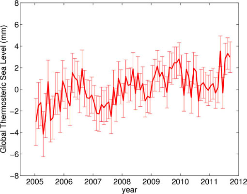FIGURE 3.2 Thermosteric sea-level rise estimated from Argo data for the upper 900 m using updated data from Leuliette and Willis (2011). The error bars are 1 standard deviation. SOURCE: Courtesy of J.K. Willis, Jet Propulsion Laboratory, California Institute of Technology.

OCR for page 33
38 SEA-LEVEL RISE FOR THE COASTS OF CALIFORNIA, OREGON, AND WASHINGTON level rates for the full ocean depth using measured rates Domingues et al. (2008) for 1961­2003 and the rela- for the upper 700 m by other investigators (Table 3.1) tively low estimates of Ishii (personal communication, and the Domingues et al. (2008) value for the deep ocean 2011) for 1961­2008 for the upper 700 m. The treat- below 700 m (Table 3.2). For the longer observational ment of data in unsampled and undersampled regions period (approximately five decades), the committee cal- of the world's oceans also can introduce uncertainties culated rates ranging from 0.5 ± 0.12 mm yr-1 (based on (Purkey and Johnson, 2010). Sampling problems are Ishii and Kimoto, 2009) to 0.59 ± 0.11 mm yr-1 (based particularly acute in the Southern Ocean and likely on Ishii, personal communication, 2011). These rates result in estimates of thermosteric sea-level rise that are are lower than the Domingues et al. (2008) rates, but biased low (Gille, 2008; Church et al., 2010). they are comparable within errors. For the post-1993 observational period, the committee's calculated rates are Models 1.0 ± 0.19 mm yr-1 and 1.43 ± 0.31 mm yr-1 (Table 3.2). The most recent estimate of Ishii (personal communica- The warming observed in the upper ocean also has tion, 2011) is comparable to estimates of Domingues et been inferred from ocean-atmosphere climate models. al. (2008) and Church et al. (2011), within their reported For example, Pierce et al. (2006) found general con- errors. sistency between models and observations for ocean The above estimates of the global thermosteric warming, with the signal disappearing around 600 m sea-level trend and its variability on interannual and depth. Climate model simulations also suggest heat up- decadal timescales differ, sometimes substantially. For take by the deep ocean (Katsman and van Oldenborgh, example, Domingues et al. (2008) shows a continued 2011; Meehl et al., 2011). Song and Colberg (2011), thermosteric sea-level rise after 2004, whereas Levitus using an ocean general circulation model constrained et al. (2009) and Ishii and Kimoto (2009) show a by sea-surface temperature and atmospheric radia- plateau (top panel of Figure 3.1). These differences tion measurements, found a strong warming signal of result from uncertainties in the data and the choice 1.1 mm yr-1 below 700 m for the 1993­2008 period. of instrument bias corrections, processing approach, This value is much higher than observational estimates baseline mean climatology, mapping technique, and (Purkey and Johnson, 2010; Kouketsu et al., 2011; Loeb treatment of unsampled or undersampled areas. Cor- et al., 2012), for reasons that are currently under debate. recting for XBT fall-rate bias reduced the errors in the thermosteric sea-level trend (S. Levitus, personal Data Assimilation communication, 2011). However, uncertainties in the bias corrections remain the dominant source of error, Ocean data assimilation techniques can be used especially for recent decades (Ishii and Kimoto 2009; to obtain estimates of deep-ocean warming and the Willis et al., 2009; Gouretski and Reseghetti, 2010; resulting thermosteric sea-level rise by constraining Lyman et al., 2010). the numerical models with available data. There are, Different data processing approaches also may however, significant differences between the various account for some differences among thermosteric sea- data assimilation products and direct observations, level estimates, such as the relatively high estimates of arising in part from uncertainties in direct observa- TABLE 3.2 Committee Estimates of Thermosteric Sea-Level Rise for the Full Ocean Depth Data Source Used in the Estimate Period Thermosteric Sea-Level Rise Estimates, This Report (mm yr-1)a Ishii and Kimoto (2009) 1951­2005 0.5 ± 0.12 Kuo and Shum (personal communication, 2011) 1955­2009 0.53 ± 0.14 Ishii (personal communication, 2011) 1961­2008 0.59 ± 0.11 Ishii and Kimoto (2009) 1993­2005 1.43 ± 0.31 Ishii (personal communication, 2011) 1993­2009 1.0 ± 0.19 aCalculated from estimates of the upper 700 m of the ocean by various investigators and the Domingues et al. (2008) rate of 0.2 ± 0.1 mm yr-1 for the deep ocean below 700 m.

OCR for page 33
CONTRIBUTIONS TO GLOBAL SEA-LEVEL RISE 39 tions and differences in data-assimilation approaches mate Experiment (GRACE) and altimeter data for estimating the state of the ocean (e.g., Church et (e.g., Lombard et al., 2007; Cazenave et al., 2009). al., 2010). The Simple Ocean Data Assimilation model Satellite altimetry measures the total sea-level change (Carton et al., 2005; Carton and Giese, 2008) uses a (steric plus ocean mass) and GRACE measures ocean multivariate sequential approach to force the ocean mass change. The difference between the two measure- model toward observed temperature and salinity data. ments provides an independent estimate of the steric Ocean dynamics and other properties are not preserved. sea-level change. However, estimates made this way Using this approach, the estimated thermosteric sea- vary significantly. level trend from 1968 to 2001 is similar to the observed estimates (Figure 3.1). Kohl and Stammer (2008) used Summary a more sophisticated approach, which synthesizes the observed data into a dynamically consistent model The thermal expansion estimates in the IPCC using the adjoint assimilation technique. To ensure Fourth Assessment Report were made before tem- dynamical consistency, the model forcing fields are perature biases due to the XBT and MBT depth errors modified. The estimated thermosteric sea-level trend were discovered. Efforts to improve the IPCC (2007) using this method shows a large decrease until 1975 estimates have focused on using new temperature and then a larger rise afterward (Figure 3.1). data, correcting instrument bias, and improving data Ocean data assimilation has been an active research processing methods. New estimates of thermosteric topic only since the 1990s. Over time, it may become sea-level rise are generally higher than those estimated a more reliable source for studies of decadal sea-level by the IPCC (2007) for the past four or five decades variability and change (Church et al., 2010). and generally lower than those estimated by the IPCC (2007) for the past 10­15 years (Figure 3.3). However, Satellites the new estimates overlap significantly with the IPCC (2007) estimates, within errors. 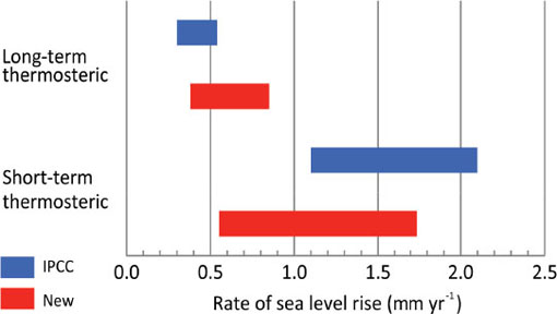A few investigators have inferred global steric Estimates of thermosteric sea-level rise for the sea-level rise from the Gravity Recovery and Cli- upper 700 m of the ocean have lower uncertainties than FIGURE 3.3 Comparison of thermosteric sea-level estimates for the full ocean depth from IPCC (2007; blue) and subsequent esti- mates (red). The bars represent the highest and lowest estimates. Long-term trends are for 1961­2003 (IPCC) and 1951­2005 (new estimates); short-term trends are for 1993­2003 (IPCC) and 1993­2008 (new estimates). SOURCE: IPCC estimates from Bindoff et al. (2007); new estimates are from Tables 3.1 and 3.2 based on data from Domingues et al. (2008), Ishii and Kimoto (2009), and Church et al. (2011).

OCR for page 33
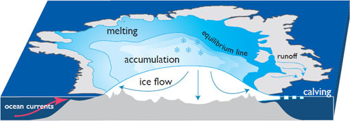
40 SEA-LEVEL RISE FOR THE COASTS OF CALIFORNIA, OREGON, AND WASHINGTON melting u eq il i b r iu m li n e runoff accumulation ice flow calving ocean currents FIGURE 3.4 Glacier and ice sheet mass balance components. Ice accumulates at high elevations and is lost at lower elevations through melting, sublimation, or iceberg calving. The boundary between areas of net gain and loss is called the equilibrium line. estimates for the full ocean depth due to the paucity caps, and ice sheets typically gain mass through snow of deep-ocean measurements. Studies suggest that accumulation and lose mass through melting and run- sampling problems cause a low bias in upper-ocean off (ablation), iceberg calving, and, to a lesser extent, thermosteric sea-level rise estimates, and also make sublimation and wind erosion and transport. Calving it difficult to assess the uncertainty in the deep-ocean can be the dominant mechanism of mass loss, account- thermosteric sea-level rise. Data assimilation and ing for 50­100 percent of the loss on the Antarctic Ice model results are not yet robust enough to be used to Sheet, about 50 percent of the loss on the Greenland fill in missing data. Ice Sheet (Rignot and Jacobs, 2002; van den Broeke et al., 2010), and, where it has been measured, about GLACIERS, ICE CAPS, AND ICE SHEETS 50 percent of loss from ocean-terminating ice cap complexes (Blaszczyk et al., 2009). In general, mass is Loss of land-based ice is a major contributor to gained at higher elevations and on the upper surface of global sea-level rise, equal to or exceeding the contri- a glacier or ice sheet, and mass is lost at lower elevations bution of thermal expansion. The equivalent of at least and at the base. The difference between accumulation 65 m of sea level is stored in glaciers, ice caps, and ice and ablation is called the mass balance, and it is deter- sheets. The Greenland and Antarctic ice sheets store the mined through a combination of in situ and satellite equivalent of about 7 m and 57 m of sea level, respec- measurements (Box 3.2), often combined with models. tively (Bamber et al., 2001; Zhang et al., 2003),1 and To determine the contributions of land ice to glaciers and ice caps store the equivalent of 0.6 ± 0.07 m, sea-level rise, mass balance estimates are converted about one-third of which is around the periphery of to sea-level equivalent (SLE), the change in global Greenland and Antarctica (Radic and Hock, 2010). average sea level that would occur if a given amount of The response of glaciers and ice sheets to climate water or ice were added to or removed from the oceans. change depends on processes acting at the upper SLE is computed by dividing the observed mass change surface; at the base, where glacial meltwater and the of the ice by the surface area of the world's oceans properties of the bedrock affect the rate of ice flow; and, (362 × 106 km2). When working with changing ice vol- in some locations, at the marine margin, where iceberg ume (e.g., rates of iceberg flux), the volume is converted calving and melting occur (Figure 3.4). Glaciers, ice to mass using the density of ice (900 kg m3). Using these values, 1.11 km3 ice = 1 km3 of water = 109 kg 1See also data compiled for the Sea-level Response to Ice Sheet water = 1 GT water, and 362 GT water = 1 mm SLE. Evolution (SeaRISE) assessment project, .

OCR for page 33
CONTRIBUTIONS TO GLOBAL SEA-LEVEL RISE 41 BOX 3.2 Measuring the Earth's Ice Monitoring the world's land ice masses is a challenging task complicated by the size, wide distribution, and generally remote and hostile envi ronments in which most glaciers are located. Changes in glacier or ice sheet volume can be calculated by mass budget methods (balancing input and output fluxes), by repeated geodetic measurements, by combinations of the two, and by measurements of mass change through gravity surveys using the GRACE satellite system. Quantitative determination of glacier and ice sheet mass balance requires a variety of data sets, including ice surface elevation and ice thickness, the rate of ice flow, and the rate of ice (snow) accumulation and ablation. Measurements are made both in situ (ideal for individual glaciers and process studies) and remotely (ideal for covering large regions). Satellite remote sensing instruments collect data at visible, near-infrared, and microwave wavelengths and may image the surface in blocks or along the ground track below the satellite (see the review in Quincey and Luckman, 2009). Ice Thickness. The thickness of glaciers and ice sheets is generally measured using radar sounding from aircraft or at the ice surface. The 25­400 MHz radar signal penetrates to the bedrock below the ice, and the difference between returns from the upper and lower surfaces is used to calculate the ice thickness. Radar sounding works best in cold, clean ice. Ice with substantial fractions of liquid water or crevasses scatter radar energy, creating com- plications for radar soundings of fast-moving outlet glaciers, especially those in warmer environments. Surface Topography. Topography is measured using aerial photogrammetry, airborne and satellite laser altimetry, and satellite radar altimetry. Radar altimeters on satellites (ERS-1, -2, Envisat, and CryoSat-2) are used to measure ice sheet surface elevation with decimeter accuracy, but the footprint of the sensor (the area on the surface within the field of view of the antenna) is relatively large (a few kilometers) and varies with surface roughness and slope. Laser altimeters have much smaller footprints (tens of meters; about 70 m for NASA's Geoscience Laser Altimeter) and may be mounted on aircraft or on satellites. Laser altimeters mounted on small aircraft are used for repeat surveys of glaciers in Alaska, where optimal flight lines are poorly suited for satellite orbital paths (Larsen et al., 2007). Repeat mapping of surface topography can be used to derive volume change, as long as neither the density nor the bed topography change between surveys. Ice Velocity. The rate of ice flow can be calculated using repeated measurements of the locations of features, either a survey monument or a natural feature (e.g., a crevasse intersection), on the ice surface. Locations can be determined using ground-based optical survey measurements, Global Posi- tioning System surveys, photogrammetry, or satellite image processing. Ice flow also can be determined from radar interferometry (e.g., Figure), which uses the change between observations in the phase of the returning radar wave to make a high-precision measurement of ground displacement relative to the spaceborne radar. Gravity. Ice sheet mass changes since 2002 can be determined from the GRACE satellite system (see Box 2.4). The ice sheet changes must be sepa- rated from other mass change signals such as those caused by glacial isostatic adjustment. In some instances the modeled corrections are robust, but in others the uncertainties can be large. The spatial resolution of the measurements depends on details of the processing and the latitude of interest (Wahr et al., 2004). Mass Balance. Accumulation and ablation are traditionally determined using in situ measurements made at least twice yearly, at the end of the ac- cumulation season and ablation season. This technique remains the only way to make direct observations of the components of the mass budget, but it is too time consuming and expensive to be used as an operational tool on the ice sheets. Accordingly, remote sensing methods are used extensively, with reliance on limited point climate and meteorological observations and on meteorological and surface energy balance models. Snow accumulation can be estimated from atmospheric models coupled with satellite observations or by analyzing annual layers in ice cores and interpolating between core sites using radar sounding of the ice layers. Melt can be estimated using energy balance models driven by atmospheric models. Runoff cannot be measured remotely, and in most cases is determined solely by modeling. continued

OCR for page 33
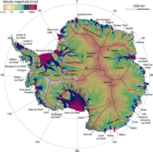
42 SEA-LEVEL RISE FOR THE COASTS OF CALIFORNIA, OREGON, AND WASHINGTON BOX 3.2 Continued FIGUREAntarctic glacier velocity (in m yr-1) derived from radar interferometry. Black lines delineate major ice divides. Velocities can reach a few km yr-1 on fast-moving glaciers (e.g., Pine Island) and floating ice shelves. SOURCE: Rignot et al. (2011b).

OCR for page 33
CONTRIBUTIONS TO GLOBAL SEA-LEVEL RISE 43 correction term is added to account for the ice volume Recent Results below the water line that has already affected sea level by its presence. On sufficiently long timescales, a cor- Since the IPCC Fourth Assessment Report was rection for glacial isostatic adjustment of the underlying published, more observations are available, and rapid bedrock, based on forward models, also may be made. flow changes at marine margins of ice sheets and gla- The conversion of ice mass loss to SLE assumes ciers, which were recognized but not included in the that all land ice melt enters the ocean. Land storage IPCC (2007) projections, are now represented in of ice melt may be significant for land-terminating some projections. Ice sheet velocity and mass balance glaciers in continental interiors (e.g., high mountains distributions are now better mapped, but the potential in Asia), but its occurrence is unconfirmed. SLE is a for rapid future increases in calving losses from ocean- globally uniform value and thus may be higher or lower terminating outlet glaciers is still poorly understood, in than the sea-level value in any particular region. part because of inadequate knowledge of the underlying physics. Estimates from the IPCC Fourth Assessment Report Glacier and Ice Cap Assessments The IPCC Fourth Assessment Report estimated that losses from glaciers and ice caps contributed Owing to the delay in assimilation of new observa- 0.58 ± 0.18 mm yr-1 to sea-level rise from 1961 to 2003 tions and the incomplete but evolving glacier inventory, and 0.77 ± 0.22 mm yr-1 from 1993 to 2003 (Bindoff most post-IPCC (2007) assessments of glacier and ice et al., 2007), with the most rapid ice losses occurring cap change (Table 3.3) are based on data collected prior in Patagonia, Alaska, northwest United States, and to 2007. The various analyses span different periods southwest Canada (Lemke et al., 2007). Uncertainties and use different methods to average sparse data and in the net loss rate were significant, however, because of to scale up regionally heterogeneous trends to estimate sparse point observations and incomplete knowledge of the global total, resulting in significant uncertainties. global glacier area and volume distribution for upscal- Estimated rates of ice loss, expressed as SLE, vary in ing point observations. On the Greenland Ice Sheet, time and space. For example, gravity observations in- the IPCC (2007) found that mass was gained at high dicate that the rate of mass loss in the Gulf of Alaska elevations because of increasing snowfall, and mass decreased from 2004 to 2008 (Luthcke et al., 2008; was lost near the coast because of increases in melting Table 3.3), but increased in the Canadian Arctic over and in the flow speed of outlet glaciers. The IPCC a similar interval (Gardner et al., 2011). These patterns estimated that the Greenland Ice Sheet contributed reflect the influence of rapid changes in the rate of ice 0.05 ± 0.12 mm yr-1 to sea-level rise from 1961 to 2003 flow (rapid dynamical response) associated with ice- and 0.21 ± 0.07 mm yr-1 from 1993 to 2003. Changes in ocean interaction in coastal regions. Antarctica were more challenging to interpret because The most recent published compilation (Cogley, of the relatively small changes in snow accumulation 2012), and the only one to use data from after 2007, rates (Monaghan et al., 2006) and to different trends shows a substantial decrease in glacier and ice cap in the flow of individual West Antarctic outlet streams. loss rates from 1.41 mm yr-1 SLE for 2001­2005 to The IPCC estimated that the Antarctic Ice Sheet con- 0.92 mm yr-1 for 2005­2010. The cause of this decrease tribution was between -0.28 and +0.55 mm yr-1 from is unclear, but suggests the potential for significant 1961 to 2003 and between -0.14 and +0.55 mm yr-1 variability on 5- to 10-year timescales and highlights from 1993 to 2003, allowing for the possibility that the the difficulty of extracting meaningful trends from Antarctic mass change may have reduced sea-level rise, short-term observations. Jacob et al. (2012) determined especially prior to 1993 (Bindoff et al., 2007; Lemke et an overall loss rate for global glaciers and ice caps of al., 2007). The rate of ice loss appears to have increased 0.41 ± 0.08 mm yr-1 for 2003­2010, but this value does since 1993 because of increasing surface melt on the not include the glaciers and ice caps on the periphery of Greenland Ice Sheet and faster flow of some outlet the Greenland and Antarctic ice sheets. They estimated glaciers in both Greenland and Antarctica. the contribution of these peripheral glaciers and ice

OCR for page 33
44 SEA-LEVEL RISE FOR THE COASTS OF CALIFORNIA, OREGON, AND WASHINGTON TABLE 3.3 Estimates of Glacier and Ice Cap Sea-Level Equivalent Sea-Level Equivalent Source Period Region Method (mm yr-1) Global Estimates IPCC (2007) 1993­2003 Global Combination of various estimates 0.77 ± 0.22 1961­2003 0.58 ± 0.18 Leclercq et al. (2011) 1850­2005 Global Glacier length 0.06 ± 0.01 Kaser et al. (2006) 2001­2004 Global Combination of three independent methods: Cogley 0.98 ± 0.19 (2009), Dyurgerov (2010), and Ohmura (2004) Cogley (2009) 2001­2005 Global Spatial polynomial interpolation 1.41 ± 0.20 Dyurgerov (2010) 2002­2006 Global Area weighting 0.95 ± 0.05 Cazenave and Llovel (2010) 2003­2007 Global Uncertainty-weighted average of available estimates 1.03 ± 0.06 Cogley (2012) 2005­2009 Global Spatial polynomial interpolation 0.92 ± 0.05a Jacob et al. (2012) 2003­2010 Global GRACE 0.41 ± 0.08b Regional Estimates Matsuo and Heki (2010) 2003­2009 High mountain Asia GRACE 0.13 ± 0.04 Jacob et al. (2012) 2003­2010 High mountain Asia GRACE 0.01 ± 0.05 Luthcke et al. (2008) 2004 Gulf of Alaska GRACE 0.39 ± 0.06 2007 0.13 ± 0.06 Gardner et al. (2011) 2004 Canadian Arctic GRACE 0.09 ± 0.02 2006 0.25 ± 0.03 a Representative of 2005/6­2009/10, but reports for the 2009/10 balance year are still incomplete. Value updated from Cogley (2012) and upscaled to all glaciers, including peripheral glaciers surrounding the ice sheets, using the method of Kaser et al. (2006). b Value excludes peripheral glaciers surrounding the Greenland and Antarctic ice sheets. Estimated loss rate (SLE), including peripheral glaciers given in Jacob et al. (2012), is 0.63 ± 0.23 mm yr-1. caps using a simple adjustment factor and arrived at a 2003 and 1998­2003, but Matsuo and Heki (2010) global total of 0.63 ± 0.23 mm yr-1, assigning substan- arrived at their value by assigning 0.027 mm yr-1 SLE tially less confidence in this rate than in the rate without (10 GT yr-1) to groundwater extraction. This may be an peripheral glaciers and ice caps. underestimate of groundwater extraction, given that the Glaciers in high mountain Asia (more than region includes the plains south of the Himalayas and 110,000 km2 of glacier area, including the Himalayas, part of the region where Tiwari et al. (2009) saw losses Karakoram, Pamirs, Caucasus, and Tien Shan regions) of ~54 GT yr-1 for 2002­2008. If a larger groundwater have experienced losses in recent decades, but the re- extraction signal were used, the GRACE data used by gion is sparsely observed and uncertainties are generally Matsuo and Heki (2010) would indicate a smaller high large. Shortly after the publication of the IPCC Fourth mountain Asia glacier loss rate. The most recent and Assessment Report, which contained an error concern- detailed analysis of high mountain Asia is presented in ing the disappearance of Himalayan glaciers, several Jacob et al (2012), who found a much lower total loss other erroneous reports were published, all based in rate of 4 ± 20 GT yr-1 for 2003­2010, corresponding part on gray literature and media stories. These created to 0.01 ± 0.05 mm yr-1 SLE. The authors ascribe the considerable confusion about the state of glaciers in the difference between their totals and other GRACE Himalayas and their near-term fate (see the summary analyses (e.g., Matsuo and Heki, 2010) to better treat- in Cogley et al., 2010). Subsequent analyses continue ment of mass concentration (mascon) calculations in to show substantial uncertainties, however. Matsuo and the GRACE processing and improved removal of the Heki (2010) used GRACE gravity methods to deter- terrestrial groundwater signal through modeling. mine ice losses from high mountain Asia and estimated All glacier and ice cap loss rates reported to date that the sea-level contribution of the entire region was are based on a global glacier and ice cap inventory 0.13 ± 0.04 mm yr-1 SLE for 2003­2009. This value that represents only ca. 48 percent of the world's was somewhat higher than the loss rate of 0.10 mm yr-1 704 ± 56 × 103 km2 of glacier-covered area exclusive determined by Dyurgerov and Meier (2005) for 1993­ of the ice sheets (Figure 3.5). The Randolph Glacier

OCR for page 33
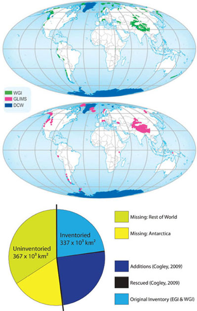
CONTRIBUTIONS TO GLOBAL SEA-LEVEL RISE 45 FIGURE 3.5 (Top) Map coverage of global glacier inventories--including the World Glacier Inventory (WGI), Global Land Ice Measurements from Space (GLIMS), and Digital Chart of the World (DCW)--used in published assessments. The figure shows the status prior to publication of the Randolph Glacier Inventory. SOURCE: United Nations Environment Programme, . (Bottom) Completeness of global glacier and ice cap inventories used in published assessments. Approximately one-third of the uninventoried area is in the peripheral glaciers and ice caps surrounding the two ice sheets, and most of the rest is in North America. "Missing" indicates that data are absent in the Cogley (2009) extended inventory. SOURCE: Cogley (2009).

OCR for page 33
46 SEA-LEVEL RISE FOR THE COASTS OF CALIFORNIA, OREGON, AND WASHINGTON Inventory, a new, complete inventory providing 100 Ice Sheet Assessments percent coverage of glaciers and ice caps, including those on the peripheries of ice sheets, has recently Systematic assessments of ice sheets began in the been completed.2 Several groups are working to update mid 1980s (e.g., Bindschadler, 1985; Oerlemans, 1989). present-day analyses and projections using the new With each assessment, the mass balance has become inventory. The glacier and ice cap loss rates presented increasingly negative (i.e., net mass loss) in both here are likely to change once the new inventory is fully Greenland and Antarctica. A number of ice sheet as- incorporated into assessments. sessments have been published since the IPCC Fourth In addition to deficiencies in the global glacier Assessment Report (Table 3.4). Methods for measur- and ice cap inventory, measurements of mass balance ing ice sheet mass balance are comparable to those terms are sparse (Dyurgerov, 2002; Kaser et al., 2006). used for glacier mass balance. Since 2002, however, Observations of glacier variations extend back into the detection of mass change using the GRACE satellite 18th century, but in situ mass balance measurements system has become a widely used tool for ice sheet mass that reveal climatic patterns do not begin until the balance owing to the operational difficulties of other early- to mid-20th century, and most records are less measurement methods over large areas. Interpretation than a few decades long (Zemp et al., 2009). As a result, of GRACE data is complicated by its intrinsic mixing scaling methods have been developed to translate local of gravity signals (Box 3.2). Glacial isostatic adjust- measurements to a global estimate (Bahr et al., 1997; ment must be corrected by modeling the lithospheric Dyurgerov, 2002; Kaser et al., 2006; Cogley, 2009). The response to loading changes (Velicogna and Wahr, incomplete inventory and the small number of long-term 2006a,b; Tregoning et al., 2009), but other mass change observational mass balance records worldwide are the terms (e.g., changes in terrestrial water storage) are largest (and hardest to quantify) sources of uncertainty smaller on the ice sheets than elsewhere. in present-day rates of glacier and ice cap mass loss. As shown in Table 3.4, the reported rates of mass Differences in methodology and in error reporting loss vary substantially, in part because of different make quantitative comparison of the various mass bal- uncertainties among measurement methods and im- ance estimates difficult. Slangen and van de Wal (2011) provements in the analysis of GRACE data. In addi- found that projections of future change in these systems tion, the ice sheet loss rates appear to experience not were about equally sensitive to uncertainty in the glacier only a long-term trend toward faster losses but also inventory as to the scaling factor used to relate tempera- significant interannual and multi-annual variability, so ture change to mass imbalance. Cazenave and Llovel measurements made over different time intervals can (2010) combined all available estimates to arrive at an be difficult to compare. The brevity of the record and uncertainty-weighted average of 1.03 ± 0.06 mm yr-1 differences in the spatial coverage, the quantities used SLE from glaciers and ice caps, or approximately to infer mass change, and the treatment of data gaps 41 percent of the total observed sea-level rise for the further complicate comparisons and trend assessment. 2003­2007 period. The committee estimated ice sheet loss rates for the Computing mean SLE rates using the published most recent period reported (2002­2009) by making a literature requires time series data and knowledge of weighted average of the values in Table 3.4.3 The aver- the uncertainties associated with the various estimates. age loss rates for 2002­2009 were 0.56 ± 0.13 mm yr-1 Such information is not always available or presented for the Greenland Ice Sheet and 0.37 ± 0.14 mm yr-1 for in a useful way. In this sense, the best mass balance the Antarctic Ice Sheet. compilation available is Cogley's (2009) glacier and ice cap data set (updated in Cogley, 2012, but released as 3 For each year, all available published values are weighted this report was being completed). For the most recent according to assessed confidence in the quality of the particular estimate, and then averaged. Some studies provide yearly values period (2005­2009), the loss rates reported for glaciers for their respective reporting periods; others provide only average and ice caps are 0.92 ± 0.05 mm yr-1. values over a multi-year period, and in these cases, the average rate was assumed to apply in each year in the interval. For a multi-year interval, the weighted average is obtained through a simple linear 2 See . average of the annual averages in that interval.

OCR for page 33
CONTRIBUTIONS TO GLOBAL SEA-LEVEL RISE 47 TABLE 3.4 Estimates of Sea-Level Equivalent from Ice Sheet Mass Loss Source Period Method Sea-Level Equivalent (mm yr-1) Greenland Ice Sheet IPCC (2007) 1993­2003 Combination of various estimates 0.21 ± 0.07 1961­2003 0.05 ± 0.12 Rignot et al. (2011a) 1992­2000 Mass balance method + GRACE 0.14 ± 0.14 2000­2003 0.47 ± 0.14 2003­2007 0.68 ± 0.14 Velicogna (2009) 2002­2003 GRACE 0.38 ± 0.09 2007­2009 0.79 ± 0.09 Schrama and Wouters (2011) 2003­2010 GRACE 0.55 ± 0.05 Cazenave et al. (2009) 2003­2008 GRACE 0.38 ± 0.05 Luthcke et al. (2008) 2004­2009 GRACE 0.52 ± 0.20 Zwally et al. (2011) 1992­2002 ICESAT 0.02 ± 0.01 2003­2007 0.47 ± 0.01 Sørensen et al. (2011) 2003­2008 ICESAT 0.58 ± 0.06 Wu et al. (2010) 2002­2008 GRACE + GPS 0.29 ± 0.06 Rignot et al. (2008) 1960s Mass balance method 0.30 ± 0.19 1970s­1980s 0.08 ± 0.14 van den Broeke et al. (2009) 2000­2008 Mass balance method 0.46 2003­2008 0.66 Antarctic Ice Sheet IPCC (2007) 1993­2003 Combination of various estimates 0.21 ± 0.35 1961­2003 0.14 ± 0.41 Rignot et al. (2011a) 1992­2000 Mass balance method + GRACE 0.18 ± 0.25 2000­2003 0.46 ± 0.25 2003­2007 0.56 ± 0.25 2007­2010 0.71 ± 0.25 Velicogna (2009) 2002­2003 GRACE 0.29 ± 0.20 Chen et al. (2009) 2002­2003 GRACE 0.52 ± 0.21 Cazenave et al. (2009) 2003­2008 GRACE 0.55 ± 0.06 Wu et al. (2010) 2002­2008 GRACE 0.23 ± 0.12 Wingham et al. (2006) 1992­2003 Radar altimetry 0.07 ± 0.08 Rapid Dynamic Change Peninsula, and the Amundsen Sea sector of the West Antarctic Ice Sheet. Warming ocean water appears to The possibility of rapid dynamic response to envi be increasing the rates of calving and melting (e.g., ronmental change as a mechanism of rapid sea-level Holland et al., 2008; Nick et al., 2009; Straneo et al., rise is a long-standing idea in glaciology (Mercer, 1978; 2010; Motyka et al., 2011), which in turn changes the Thomas and Bentley, 1978). Rapid flow processes have coupling between glacier ice and the adjacent bedrock, been observed on ice sheets (e.g., Bentley, 1987) and increasing the rate of ice flow. In some extreme cases, at marine-terminating glaciers for many years (Meier the discharge speed increased by an order of magnitude and Post, 1987). Increases in the rate of rapid transfer at glacier termini, although the rate of change varied of ice from land to the ocean by glacier flow and iceberg from year to year (e.g., Joughin et al., 2004; Howat calving were observed in Greenland between ca. 1995 et al., 2007). Climate-driven changes in sea ice in and 2005 (e.g., Rignot and Kanagaratnam, 2006) and the coastal fjord environment may also be important in Antarctica. These observations were published late in (Amundson et al., 2010). Rapid changes at the outlet the compilation of results for the IPCC Fourth Assess glacier terminus propagate into the interior over time ment, so the report included the observations, but not scales and with magnitudes that depend on both the an extensive analysis or interpretation. climate and glacier dynamics (Pfeffer, 2007). Ice sheet A variety of observational studies are now available mass balance over the next century depends in part on which, together with process studies, suggest a small how far and how rapidly that propagation proceeds (see set of underlying causes for changes in outlet glacier "Recent Global Sea-Level Projections" in Chapter 5). flow around the Greenland Ice Sheet, the Antarctic

OCR for page 33
48 SEA-LEVEL RISE FOR THE COASTS OF CALIFORNIA, OREGON, AND WASHINGTON The position of the grounding line--the transition West Antarctica is possible in some warming scenarios, at which ice resting on bedrock goes afloat--depends such as four times the preindustrial carbon dioxide on the ice thickness and varies with the ice flux through (Ridley et al., 2010) or 5°C ocean warming (Pollard the transition zone. Regions where the base of the ice and DeConto, 2009), but requires thousands of years rests below sea level and the grounding line is relatively (e.g., Marshall and Cuffey, 2000; Pollard and DeConto, unprotected by adjacent floating ice are the most vul- 2009; Ridley et al., 2010). nerable to rapid acceleration and thinning (Thomas et The rapid dynamic response from glaciers outside al., 1979; Scambos et al., 2004; Schoof, 2007). Rapid the ice sheets is less important than ice sheet dynamics retreat is possible where the bed is below sea level over the long term because glaciers do not contain and slopes down toward the interior because both the significant volumes of marine-grounded ice. However, thickness of the ice, and thus ice flux, and the thickness the potential for significant short-term contributions required to overcome buoyancy increase in the inland is large. Between 1996 and 2007, Columbia Glacier, direction (Pfeffer, 2007; Schoof, 2007). on Alaska's south coast, lost mass at an average rate of Despite rapid changes along the margins of the 6.80 GT yr-1, or 0.019 mm yr-1 SLE, approximately Greenland and Antarctic ice sheets, it is unlikely that 0.7 percent of the rate of global sea-level rise during the ice sheets will disappear over the next millennium. this period (Rasmussen et al., 2011, corrected here for The ice sheets are so thick (Figures 3.6 and 3.7) that ice already grounded below sea level). The volume of much of the surface is in higher, relatively cooler parts Columbia Glacier, approximately 150 km3, is too small of the atmosphere, allowing a positive mass balance to to contribute to sea level at such a rate for long, but be maintained even as the climate warms. However, if marine-terminating glaciers of this size can be signifi- dynamic thinning reduced the Greenland Ice Sheet, for cant factors on decadal scales. example, below some threshold size, winter snow would not compensate for the loss and the ice sheet would not Summary re-grow under current climate conditions (Toniazzo et al., 2004; Ridley et al., 2010). 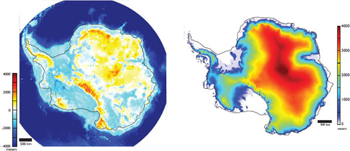Studies of such thresholds Most post-IPCC (2007) assessments of glacier and suggest that widespread denudation of Greenland and ice cap change have been made using data collected 4000 3000 4000 2000 2000 1000 0 500 km 0 -2000 meters 500 km -4000 meters FIGURE 3.6(Left) Antarctic bedrock elevations. Transition from light blue to dark blue marks the edge of the continental shelf. (Right) Antarctic surface elevations. Black line marks the approximate edge of the present-day ice (floating and grounded). Areas where the bed of the ice sheet is below sea level (e.g., West Antarctic Ice Sheet) are expected to be more vulnerable to rapid change than regions where the bed is above sea level. SOURCE: Data from Le Brocq et al. (2010).

OCR for page 33
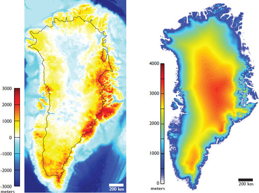
CONTRIBUTIONS TO GLOBAL SEA-LEVEL RISE 49 4000 3000 3000 2000 1000 2000 0 -1000 1000 -2000 0 200 km -3000 200 km meters meters FIGURE 3.7 Greenland bedrock elevation (left) and surface elevation (right). Black line marks the approximate edge of the present-day ice (floating and grounded). SOURCE: Original bedrock elevation from Bamber et al. (2001), modified to include data in the Jakobshavn Isbrae region from the Center for Remote Sensing of Ice Sheets, . prior to 2007. The new estimates of the glacier and Since about 2006, the rate of ice loss in Greenland ice cap contribution to sea-level rise tend to be at the has increased substantially and the rate of change in high end of the estimates provided in the IPCC Fourth Antarctica, while more difficult to quantify, appears to Assessment Report (Table 3.3). Most new assessments have shifted from negative to positive (e.g., Vaughan, of ice sheet change are based on GRACE data, which 2006; Rignot and Kanagaratnam, 2006; Rignot et al., have been available since 2002, although a few long- 2008; van den Broeke et al., 2009; Cazenave and Llovel, term assessments have been made using mass balance 2010; see also Table 3.4). This growing contribution methods. Different methods for estimating ice-sheet arises from increases in both the amount of surface melt- mass balance yield substantially different results. Esti- ing and the rate of ice discharge through coastal outlet mates made using more recent data (Table 3.4) show glaciers. Calculated loss rates from glaciers and ice caps that the contribution of Greenland to sea-level rise is have decreased since about 2005 (Cogley, 2012), due to significantly higher than the IPCC (2007) estimate and significant short-term variability in the global glacier the contribution of Antarctica has shifted toward the loss rate signal and, to a lesser extent, to improvements positive side of the range (raising sea level). in the global glacier inventory. Short-term (pentads

OCR for page 33
50 SEA-LEVEL RISE FOR THE COASTS OF CALIFORNIA, OREGON, AND WASHINGTON to decades) glacier loss rates are strongly negative but climate models, to estimate surface boundary condi- with no clear pattern of variability, whereas the longer tions such as temperature and precipitation. Because term trend (decade to century) is consistently negative of the complexity of hydrological processes and the and accelerating. In the most recent periods reported, wide range of spatial and temporal scales involved, fully the loss rates are 0.56 ± 0.13 mm yr-1 from 2002 to deterministic models are generally not used. A variety 2009 for the Greenland Ice Sheet, 0.37 ± 0.14 mm yr-1 of nondeterministic approaches have been developed from 2002 to 2009 for the Antarctic Ice Sheet, and (Eagleson, 1994; Famiglietti et al., 2009), and efforts to 0.92 ± 0.05 mm yr-1 from 2005 to 2009 for glaciers develop deterministic, quasi-deterministic, and hybrid and ice caps. models are being pursued (e.g., Kollet and Maxwell, 2008; Wood et al., 2011). These models are strongly TERRESTRIAL WATER STORAGE dependent on observations, which are coming increas- ingly from remote sensing (Box 3.3). Water lost or gained by the continents generally The GRACE satellite system (Boxes 2.4 and 3.3) results in a corresponding gain or loss of water by provide a sensitive means of detecting changes in land the oceans. Terrestrial water is stored in soils and the water mass, provided that other confounding mass subsurface (groundwater, aquifers), in snowpack and change signals can be independently assessed and permafrost, in surface water bodies (e.g., rivers, lakes, removed. Changes in groundwater mass and biomass reservoirs, wetlands), and in biomass. Some of the can be observed at a precision necessary for detect- water withdrawn from these sources as a result of ing, for example, seasonal changes in soil moisture human activities such as groundwater pumping, wetland content. The limited spatial resolution of GRACE drainage, diversion of surface water for irrigation, and is a minor impediment to its utility in groundwater deforesta tion eventually reaches the ocean, raising sea investigations, given the distributed character of most level at global, regional, and local scales (e.g., Bindoff et al., 2007; Milly et al., 2010). Conversely, some water that would normally reach the ocean is diverted through processes such as impoundment of water behind dams, subsurface infiltration beneath dams, and infiltration of BOX 3.3 irrigation water to depths beneath the root zone, thus Terrestrial Water Measurements lowering sea level or reducing the rate of sea-level rise. Prior to the launch of the GRACE gravity experiment, changes Some changes in terrestrial water storage can be in terrestrial water storage were nearly impossible to measure evaluated with reasonable precision at local scales, directly, and the terrestrial component of the water budget was esti- including changes caused by groundwater withdrawal, mated largely by modeling. Reservoir impoundment was estimated deforestation, agriculture, wetland drainage, and reser- by tallying the construction of reservoirs. Groundwater mining was voir construction. On global scales, however, the ter- estimated, for example, by balancing population-based estimates of well water extraction with well recharge modeled using groundwater restrial water balance is far more difficult to estimate. hydrological methods. Not only must all hydrological fluxes be evaluated, but The launch of the GRACE satellite system in 2002 provided also geographic coverage of in situ measurements, such scientists with the first means to directly measure changes in the as river and stream gage records, is spotty. In some parts mass of water on the Earth's surface and in the ground. Water mass of the world, instrument coverage is even declining.4 can be determined at resolutions ranging from approximately 8 mm For example, the number of stream gages monitoring of water equivalent within a 750 km radius sample near the poles to approximately 25 mm of water equivalent near the equator (Wahr freshwater discharge into the Arctic Basin declined by et al., 2006). The principal difficulty in interpreting GRACE data 38 percent between 1985 and 2004 (Corell, 2005). for hydrological studies lies in separating out undesired signals, Terrestrial hydrologic models can be used to close including those arising from glacial isostatic adjustment (corrected observational gaps and, when coupled with global using measurements or models) and from adjacent mass changes such as glacier and ice sheet changes (addressed using processing 4 See ; .

OCR for page 33
CONTRIBUTIONS TO GLOBAL SEA-LEVEL RISE 51 groundwater storage, except in areas where confound- Groundwater Depletion ing mass change signals are immediately adjacent. Distinguishing mass losses from Himalayan glaciers In arid regions with significant populations and/ from groundwater losses in adjacent agricultural land or agricultural or industrial activity (e.g., portions of to the south, for example, requires careful processing the United States, Mexico, Australia, China, Spain, and interpretation of GRACE data. and North Africa; see Shiklomanov, 1997), the rate of groundwater extraction often exceeds the rate of recharge. Huntington (2008) compiled published es- Estimates from the IPCC Fourth Assessment Report timates of groundwater depletion, which ranged from The IPCC Fourth Assessment Report and other 0.21 mm yr-1 to 0.98 mm yr-1 SLE (Table 3.5), but the previous assessments found large interannual and time period to which this rate applies was not specified decadal fluctuations in the storage of water on land, and the estimates are geographically incomplete. Based likely associated with changes in precipitation, but no on hydrological modeling, Wada et al. (2010) estimated significant trend in land water storage due to climate global groundwater depletion of 0.35 ± 0.1 mm yr-1 change (e.g., Bindoff et al., 2007). Because land hydrol- SLE for 1960, increasing to 0.8 ± 0.1 mm yr-1 SLE ogy records are short, sparse, and poorly distributed for 2000. Milly et al. (2010), also using modeling for global calculations, the magnitude of changes in methods, estimated lower values of 0.12 mm yr-1 SLE water storage is highly uncertain. However, the average for 1981­1998, 0.25 mm yr-1 SLE for 1993­1998, magnitude of change over annual and longer time and 0.2­0.3 mm yr-1 SLE for "recent years." Milly scales during the reporting period (1961­2003) must et al. (2010) acknowledged, but did not quantify, have been small, given that the combined contribu- considerable uncertainty in their estimates. Konikow tions of land ice and thermal expansion alone nearly (2011) estimated global groundwater depletion from match observed changes in sea level since 1993. The 1900 to 2008, and found it increased significantly to IPCC Fourth Assessment Report estimated that the 0.4 mm yr-1 during 2001­2008, double the rate of the contribution of land hydrology to sea-level change was 1990s. Most recently, Wada et al. (2012a) made an <0.5 mm yr-1 (Bindoff et al., 2007). extensive assessment of groundwater extraction and depletion, arriving at a value of 0.54 ± 0.09 mm yr-1 SLE for 1993­2008. Recent Advances The terrestrial hydrologic processes contributing to Reservoir Storage sea-level change remain poorly constrained, although the importance of water storage in artificial reservoirs Until recently, additions to sea level from ground- has become increasingly clear. Apart from changes in water extraction were thought to be largely offset by precipitation patterns and land ice volume, the primary increasing reservoir storage, although few studies es- terrestrial water fluxes are now thought to be reservoir timated uncertainties in reservoir storage. Chao et al. construction, which lowers sea level, and ground (2008) estimated the water volume stored in 29,484 water depletion, which raises sea level. The continual reservoirs constructed since about 1900 using the Inter- development of processing techniques for analyzing national Commission on Large Dams' World Register data from the GRACE satellites (e.g., Ramillien et al., of Dams. Summing their stated water impoundment as 2008) as well as methods for modeling global ground- the reservoirs were constructed provided the volume of water transport (e.g., Oleson et al., 2010) have made it water impounded as a function of time. Converting to possible to more precisely determine changes in land SLE yielded a reservoir storage rate of -0.55 mm yr-1 for water storage. Several new data sets have been pub- the 20th century (Chao et al., 2008). Lettenmaier and lished since the IPCC Fourth Assessment Report, but Milly (2009) found the equivalent impoundment to be many do not specify analysis periods, making it difficult -0.35 mm yr-1 SLE for 1940­1950 (Table 3.5). Milly et to compare estimates or analyze trends. al. (2010) used results from Gornitz (2001) and others to estimate that the impoundment rate of global reser-

OCR for page 33
52 SEA-LEVEL RISE FOR THE COASTS OF CALIFORNIA, OREGON, AND WASHINGTON TABLE 3.5 Estimates of Groundwater Extraction and Reservoir Impoundment Source Period Method Sea-Level Equivalent (mm yr-1) Net terrestrial depletion IPCC (2007) 1910­1990 Synthesis of reports -1.5 1990 -1.1­+1.0 Church et al. (2011) 1993­2008 Synthesis -0.27­+0.11 Groundwater extraction IPCC (2007) None given Synthesis of reports <0.5 Huntington (2008) None given Synthesis 0.21­0.98 Wada et al. (2010) 1960­2000 Hydrologic models 0.35­0.8 Milly et al. (2010) 1981­1998 Synthesis, models 0.12 1993­1998 0.25 "Recent years" 0.2­0.3 Konikow (2011) 2001­2008 Synthesis, models 0.4 Wada et al. (2012a) 1993­2008 Synthesis, models 0.45­0.63 Reservoir impoundment Chao et al. (2008) Past half-century Model -0.55 Lettenmaier and Milly (2009) 1940­1950 Model -0.35 Milly et al. (2010) Before 1978 Synthesis, models -0.5 After 1978 -0.28 Wada et al. (2012b) 1993­2008 Update of Chao et al. (2008) with seepage correction ~-0.20­ -0.40 voir storage declined from approximately -0.5 mm yr-1 effects (e.g., changes in soil hydraulic conductivity) of SLE before 1978 to approximately -0.25 mm yr-1 SLE thawing the global permafrost area of 22 ± 3 × 106 km2 after 1978. They attributed this decrease to slowing in (Gruber, 2011) may become significant in the near the rate of reservoir construction and to sedimentation, future. Changes in global lake storage contributed which slightly offset the storage capacity of existing about +0.11 mm yr-1 to sea level during the 1992­2008 reservoirs (Figure 3.8). How much sedimentation in period (Milly et al., 2010), but paleoclimatic records reservoirs affects sea-level rise is a matter of debate. show that lake levels exhibit strong interannual and Huntington (2008) found that sedimentation results interdecadal variability, so this rate is not a good indi- in a time-dependent loss of reservoir volume, which cator of future trends. The magnitude and sometimes affects the rate of sea-level rise. On the other hand, even the sign of other land water sources to sea level, Chao et al. (2008) argued that sedimentation displaces including irrigation, wetland drainage, urbanization, water behind dams and thus should have no effect on and deforestation, are unknown (Milly et al., 2010). the contribution of reservoir storage to sea-level rise. Regardless, the effect of sedimentation is likely to be Summary small compared with the decline in the number of res- ervoirs constructed. Wada et al. (2012b) estimated that Transfers of water (excluding ice melt) between decreased dam building lowered the contribution of res- the land and oceans are dominated by groundwater ervoir storage to about 0.3 ± 0.1 mm yr-1 for 1993­2008. depletion, which raises sea level, and reservoir im- poundment, which lowers sea level. Although more Other Contributors data (e.g., GRACE) and model results are available now than were for the IPCC Fourth Assessment Re- Snow accumulation and loss dominate seasonal port, it remains difficult to constrain the contributions variations in the terrestrial water contribution to global of terrestrial water to sea-level rise and uncertainties mean sea level but do not contribute to a long-term are large. Recent estimates for groundwater depletion trend (Milly et al., 2003; Biancamaria et al., 2011). The and reservoir impoundment are in line with the IPCC effects of changes in permafrost on sea level are cur- (2007) estimates, on the order of 0.5 mm yr-1. The two rently unknown, although the secondary hydrological terms sum to near zero, within stated uncertainties. As

OCR for page 33
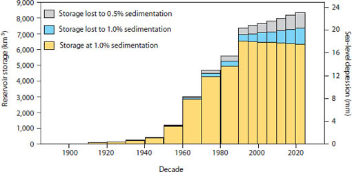
CONTRIBUTIONS TO GLOBAL SEA-LEVEL RISE 53 9,000 24 Storage lost to 0 .5% sedimentation 8,000 Storage lost to 1.0% sedimentation 20 7,000 Reservoir storage (km 3) Sea-level depression (mm) Storage at 1.0% sedimentation 6,000 16 5,000 12 4,000 3,000 8 2,000 4 1,000 0 0 1900 1920 1940 1960 1980 2000 2020 Decade FIGURE 3.8 Accumulated global reservoir water storage in dams from 1900 to 2025 (yellow bars), based on observations and projections. The rate of water storage in dams higher than 15 m or with a capacity of more than 3 million m3 has begun declining over the past decade because of sedimentation (blue and gray bars), potentially reducing the rate of sea-level rise. SOURCE: L ettenmaier and Milly (2009). this report was nearing completion, a new evaluation by In addition, new types of measurements, notably Wada et al. (2012b) found a net positive contribution to the GRACE satellite system, and expanded data sets global sea-level rise of 0.25 ± 0.09 mm yr-1 during the have become available since the IPCC Fourth Assess- 1990­2000 period as a result of a decrease in reservoir ment Report was published. Estimates incorporating construction and an increase in groundwater deple- the new data suggest a faster growing contribution of tion. If this result holds, terrestrial water storage could land ice to sea-level change than was seen in IPCC become a significant contributor to future sea-level rise. (2007) for the two periods. Since 2006, ice loss rates have accelerated in the ice sheets and declined in CONCLUSIONS glaciers and ice caps, likely reflecting interannual to multi-annual variability and possibly uncertainties The most comprehensive recent assessments of in data processing or interpretation of short records. global sea-level rise is given in the IPCC Fourth The most recent published estimate is that land ice Assess ment Report, which evaluated data and research melt accounted for about 65 percent of global sea-level results published up to about mid-2006, and Church et rise for 1993­2008 (Church et al., 2011). The prospect al. (2011), which provided updated data on the com- of increased ice sheet melting is important to future ponents of sea-level rise. The IPCC (2007) found that sea-level rise because the Greenland and Antarctic ice the relative contributions to global sea-level rise varied sheets store the equivalent of at least 65 m of sea level. over time, with thermal expansion contributing signifi- New data and models also are available for estimat- cantly more to sea-level rise for 1993­2003 than for ing the contribution of terrestrial water (besides ice 1961­2003. Since then, thermal expansion estimates melt) to global sea-level rise. Although the contribu- have been corrected for instrument biases, which gave tions of the two largest terms--groundwater depletion, systematically warmer temperatures than the true value which transfers water to the ocean and raises sea level, globally and cooler temperatures than the true value in and reservoir impoundment, which prevents water a portion of the Atlantic Ocean. The corrected rates from reaching the ocean and lowers sea level--are of thermosteric sea-level rise for the two IPCC (2007) significant, they are difficult to measure. As a result, periods are more similar, with a higher thermal expan- most recent assessments have not assigned a rate to sion contribution for 1961­2003 and a lower thermal terrestrial storage or assigned a rate of zero, within the expansion contribution for the 1993­2003 period. limits of uncertainty.

OCR for page 33