
Sea-level change is one of the most visible consequences of changes in the Earth’s climate. A warming climate causes global sea level to rise principally by (1) warming the oceans, which causes sea water to expand, increasing ocean volume, and (2) melting land ice, which transfers water to the ocean. Tide gage and satellite observations show that global sea level has risen an average of about 1.7 mm yr-1 over the 20th century (Bindoff et al., 2007), which is a significant increase over rates of sea-level rise during the past few millennia (Shennan and Horton, 2002; Gehrels et al., 2004). Projections suggest that sea level will continue to rise in the future (Figure 1.1). However, the rate at which sea level is changing varies from place to place and with time. Along the west coast of the United States, sea level is influenced by changes in global mean sea level as well as by regional changes in ocean circulation and climate patterns such as El Niño; gravitational and deformational effects of ice age and modern ice mass changes; and uplift or subsidence along the coast. The relative importance of these factors in any given area determines whether the local sea level will rise or fall and how fast it will change.
Sea-level change has enormous implications for coastal planning, land use, and development along the 2,600 km shoreline of California, Oregon, and Washington (referred to hereafter as the U.S. west coast). Rising sea level increases the risk of flooding, inundation, coastal erosion, wetland loss, and saltwater intrusion into freshwater aquifers in many coastal communities (e.g., Heberger et al., 2009, 2011). Valuable infrastructure, development, and wetlands line much of the coast. For example, significant development along the edge of central and southern San Francisco Bay—including two international airports, the ports of San Francisco and Oakland, a naval air station, freeways, housing developments, and sports stadiums—has been built on fill that raised the land level only a few feet above the highest tides. The San Francisco International Airport will begin to flood with as little as 40 cm of sea-level rise (Figure 1.2), a value that could be reached in several decades (Figure 1.1).
Coastal infrastructure and ecosystems are already vulnerable to high waves during ocean storms (e.g., Figure 1.3), especially when storms coincide with high tides and/or El Niño events. For example, a strong El Niño, combined with a series of large storms at times of high astronomical tides, caused more than $200 million dollars in damage (in 2010 dollars) to the California coast during the winter of 1982–1983 (Griggs et al., 2005). Higher sea levels and heavy rainfall caused flooding in low-lying areas and increased the level of wave action on beaches and bluffs (Storlazzi and Griggs, 2000). More than 3,000 homes and businesses were damaged, 33 oceanfront homes were completely destroyed, and roads, parks, and other infrastructure was heavily damaged. The damage will likely increase as sea level continues to rise and more of the shoreline is inundated.
In November 2008, Governor Arnold Schwarzenegger issued Executive Order S-13-08 directing California state agencies to plan for sea-level rise and coastal impacts.1 Included in the executive
__________
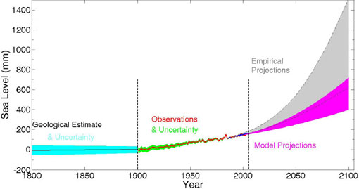
FIGURE 1.1 Estimated, observed, and projected global sea-level rise from 1800 to 2100. The pre-1900 record is based on geological evidence, and the observed record is from tide gages (red line) and satellite altimetry (blue line). Example projections of sea-level rise to 2100 are from IPCC (2007) global climate models (pink shaded area) and semi-empirical methods (gray shaded area; Rahmstorf, 2007). SOURCES: Adapted from Shum et al. (2008), Willis et al. (2010), and Shum and Kuo (2011).
order was a request that the National Research Council (NRC) establish a committee to assess sea-level rise in California to inform state planning and development efforts. Prior to release of the NRC report, the state agencies were instructed to incorporate sea-level-rise projections into their planning process. The range of projections adopted by California as interim values are 13–21 cm for 2030, 26–43 cm for 2050, and 78–176 cm for 2100 (CO-CAT, 2010).
Following the California executive order, the states of Oregon and Washington, the U.S. Army Corps of Engineers, the National Oceanic and Atmospheric Administration, and the U.S. Geological Survey joined California in sponsoring this NRC study. These agencies need sea-level information for a variety of purposes, including assessing coastal hazard vulnerability, risks, and impacts; informing adaptation strategies; and improving coastal hazard forecasts and decision support tools.
This report provides an assessment of current knowledge about changes in sea level expected in California, Oregon, and Washington for 2030, 2050, and 2100 (see Box 1.1 for the committee charge). The years for the assessment represent planning horizons: 2030 is a typical planning horizon for many local managers; 2050 is the latest date for which conventional population projections are available; and 2100 is the limit beyond which uncertainties become too high for planning.2 The report primarily focuses on how much sea level is likely to rise globally (Task 1) and along the west coast of the United States (Task 2). Processes that have only transient effects on sea level (e.g., tides, tsunamis) were considered only if the nature of the process affects trends in sea level (e.g., changes in frequency of intensity of storms [Task 2a]). Coastal impacts or measures to lessen them were considered only in the context of summarizing what is known about how coastal habitats and natural and restored environments respond to and protect against future sea-level rise and storms (Tasks 2b and 2c).
__________
2 Jeanine Jones, California Department of Water Resources, personal communication, December 3, 2008.
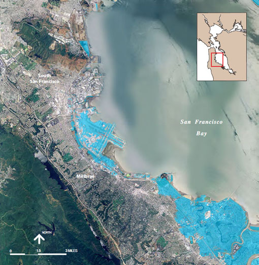
FIGURE 1.2 Expected inundation of low-lying areas, including the San Francisco International Airport (center), in the San Francisco Bay Area with a 40 cm rise in sea level (light blue shading). SOURCE: Bay Conservation and Development Commission, <http://www.bcdc.ca.gov/planning/climate_change/index_map.shtml>.
Assessments are intended to yield a judgment on a topic, based on review and synthesis of scientific knowledge. Beginning in 1989, the primary assessments of global sea-level change have been carried out by thousands of scientists working under the auspices of the Intergovernmental Panel on Climate Change (IPCC). IPCC assessments, which are made every 5 or 6 years, evaluate observations, models, and analyses of climate change, including sea-level change. For Task 1, this report summarizes the latest IPCC (2007) findings on global sea-level rise and its major components, then updates them with more recent results.
For Task 2, the committee drew on published research on sea-level change along the west coast of the United States and also carried out its own analyses. Prior assessments of the rate of local sea-level rise have been made for Washington (Mote et al., 2008)
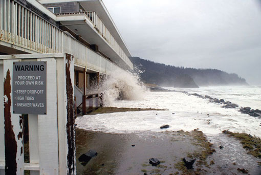
FIGURE 1.3 High surf during a high tide of nearly 2.7 m removed the front lawn of the Pacific Sands Resort at Neskowin, Oregon, on January 9, 2008. SOURCE: Courtesy of Armand Thibault.
BOX 1.1
Committee Charge
The committee will provide an evaluation of sea-level rise for California, Oregon, and Washington for the years 2030, 2050, and 2100. The evaluation will cover both global and local sea-level rise. In particular, the committee will
1. Evaluate each of the major contributors to global sea-level rise (e.g., ocean thermal expansion, melting of glaciers and ice sheets); combine the contributions to provide values or a range of values of global sea-level rise for the years 2030, 2050, and 2100; and evaluate the uncertainties associated with these values for each timeframe.
2. Characterize and, where possible, provide specific values for the regional and local contributions to sea-level rise (e.g., atmospheric changes influencing ocean winds, ENSO [El Niño-Southern Oscillation] effects on ocean surface height, coastal upwelling and currents, storminess, coastal land motion caused by tectonics, sediment loading, or aquifer withdrawal) for the years 2030, 2050 and 2100. Different types of coastal settings will be examined, taking into account factors such as landform (e.g., estuaries, wetlands, beaches, lagoons, cliffs), geologic substrate (e.g., unconsolidated sediments, bedrock), and rates of geologic deformation. For inputs that can be quantified, the study will also provide related uncertainties. The study will also summarize what is known about
a. climate-induced increases in storm frequency and magnitude and related changes to regional and local sea-level rise estimations (e.g., more frequent and severe storm surges);
b. the response of coastal habitats and geomorphic environments (including restored environments) to future sea-level rise and storminess along the west coast;
c. the role of coastal habitats, natural environments, and restored tidal wetlands and beaches in providing protection from future inundation and waves.
and California (e.g., Cayan et al., 2009), and numerous studies have been published on individual contributors to sea-level change along the U.S. west coast. The committee also analyzed tide gage records and Global Positioning System data from California, Oregon, and Washington for their local (around the station) and regional (along the coast of one or more states) trends, and extracted regional information from satellite altimetry data and glacial isostatic adjustment models.
The most challenging aspect of the committee charge was the projections of sea level for 2030, 2050, and 2100. The numerical global climate models developed for the IPCC Fourth Assessment Report3 project global sea-level rise to 2100. However, they do not account for rapid changes in the behavior of ice sheets and glaciers as melting occurs (ice dynamics) and thus likely underestimate future sea-level rise. The new suite of climate models for the Fifth Assessment Report was not available at the time of writing this report. Consequently, the committee projected global sea-level rise (Task 1) using model results from the IPCC Fourth Assessment Report, together with a forward extrapolation of land ice that attempts to capture an ice dynamics component. The committee also considered results from semi-empirical projections, which are based on the observed correlation between global temperature and sea-level change (e.g., Vermeer and Rahmstorf, 2009). For the projections of sea-level rise along the U.S. west coast (Task 2), the committee derived local values using regional ocean information extracted from global models, GPS data from along the coast, and ice loss rates of large or nearby glaciers.
Uncertainty
In the IPCC Fourth Assessment Report, the major components of global sea-level rise were estimated at the 90 percent confidence level (Bindoff et al., 2007). That is, values given as x ± e mean that there is a 90 percent chance that the true value is in the range x - e to x + e. This report follows the IPCC convention unless specified otherwise.
Uncertainty in projecting climate-related sea-level changes arises from three sources: internal variability of the climate system, which fluctuates on interannual to multidecadal and longer timescales and on regional to global spatial scales; model uncertainty; and scenario uncertainty (Hawkins and Sutton, 2009). The first is particularly important for projections based on extrapolation of observations because observational records tend to be short relative to the timescale of variability in the climate system. Models have uncertainties because they are mathematical approximations that depart in important ways from the actual system. Uncertainty in models used to describe key elements of sea-level change results from uncertainties in model parameters (e.g., initial conditions, boundary conditions) as well as structural uncertainties from incomplete understanding of some climate processes or an inability to resolve the processes with available computing resources (Knutti et al., 2010). Finally, future emissions of greenhouse gasses and other factors that drive changes in the climate system depend on a collection of human decisions at local, regional, national, and international levels, as well as potential but unknown technological developments. The IPCC deals with this uncertainty by providing a range of possible futures (scenarios) based on assumptions about trends in concentrations of greenhouses gases and other influences on the climate (e.g., Moss et al., 2010).
This report uses both model and extrapolation approaches to make projections. Each approach has different uncertainties (e.g., extrapolations take no account of emission scenarios), which were combined into a single uncertainty range for the projections. Although isolating the various sources of uncertainty may have been useful for some applications (e.g., evaluating costs and risks of various mitigation strategies), it was not required in the committee charge and would have required a different analysis approach.
Sea level is neither constant nor uniform everywhere, but changes continually as a result of interacting processes that operate on timescales ranging from hours (e.g., tides) to millions of years (e.g., tectonics). Processes that affect ocean mass, the volume of ocean water, or sea-floor topography cause sea level to change on global scales. On local and regional scales, sea level is
__________
3 More than 20 such models from around the world were analyzed and compared through the World Climate Research Program’s Coupled Model Intercomparison Project (CMIP3). See <http://www-pcmdi.llnl.gov/ipcc/about_ipcc.php>.
also affected by vertical land motions and local climate and oceanographic changes. The primary factors that contribute to global and local sea-level change are illustrated in Figure 1.4 and discussed below.
Global Sea-Level Change
Global sea level has varied significantly throughout Earth’s history. Sediment and ice-core records of these changes provide a pre-anthropogenic context for understanding the nature and causes of current and future changes. Over the past 2.5 million years, large continental ice sheets grew during long intervals of cold global temperatures (glacial periods or ice ages) and retreated during intervals of warm global temperatures (interglacial periods). Traces of paleoshorelines, found along many of the world’s coastlines, provide robust evidence that global mean sea level was at least 6 m higher during the last interglacial period (~116,000–130,000 years ago) than at present (Kopp et al., 2009). During the Last Glacial Maximum (~26,000 years ago), approximately 40 × 106 km3 of sea water was transferred to the continents and stored as ice. During that period, ice sheets covered much of North America, northern Europe, and parts of Asia, and sea levels were 125–135 m lower than present (Peltier and Fairbanks, 2006; Clark et al., 2009). The onset of deglaciation more than 20,000 years ago (Peltier and Fairbanks, 2006) caused sea level to rise at an average rate of about 10 mm yr-1 (Alley et al., 2005). Empirical and glacial isostatic modeling studies suggest that the rate of ice melt dropped significantly 7,000 years ago (Gehrels, 2010), then declined steadily to a value of zero change around 2,000 years ago (Fleming et al., 1998; Peltier, 2002b; Peltier et al., 2002). Geological data from salt marshes show a clear acceleration from relatively low rates of sea-level change during the past two millennia (order 0.25 mm yr-1; Figure 1.5) to modern rates (order 2 mm yr-1) sometime between 1840 and 1920 (Kemp et al., 2011).
Since the industrial era began, changes in global sea level have been driven in part by the accumulation of greenhouse gases in the atmosphere, which trap heat and raise global temperatures. The primary processes responsible for modern sea-level rise are thermal expansion of ocean water and melting from glaciers,
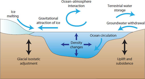
FIGURE 1.4 Processes that influence sea level on global to local scales. SOURCE: Modified from Milne et al. (2009).
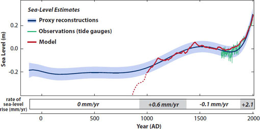
FIGURE 1.5 Sea-level estimates for the past 2000 years, adjusted for glacial isostatic effects, from proxy (geological) evidence (blue), tide gage observations (green), and Modified semi-empirical model hindcasts (red). Dotted red line shows where the model hindcast deviates from the proxy record. The lower panel shows rates of sea-level change in mm yr-1 based on the proxy reconstructions. SOURCE: Data from Jevrejeva et al. (2008), Vermeer and Rahmstorf (2009), and Kemp et al. (2011).
ice caps, and the Greenland and Antarctic ice sheets (Figure 1.6). Changes in the amount of water stored in land reservoirs have a smaller effect on global sea level. In general, groundwater extraction transfers water to the ocean and causes sea level to rise, and filling of land reservoirs causes sea level to fall.
Local and Regional Sea-Level Change Along the U.S. West Coast
Relative (or local) sea level is the mean level of the sea with respect to the land, both of which change with time, as summarized below.
Changes in Ocean Levels
Sea level in the Pacific Ocean is affected by ocean circulation, short-term climate variations, storms, and gravitational and deformational effects of land ice changes. Changes in ocean circulation affect regional sea level on seasonal to decadal and longer timescales by redistributing ocean mass and altering seawater temperature and salinity patterns. These changes in ocean circulation are driven primarily by changes in winds and ocean surface density associated with the El Niño-Southern Oscillation (ENSO), which has a period of 2 to 7 years, and the Pacific Decadal Oscillation, which has a typical period of several decades. During a strong El Niño, a pulse of warm water in the eastern equatorial Pacific moves northward, forming a bulge in sea level along the California, Oregon, and Washington coasts. The low atmospheric pressures and west-southwest winds induced by an El Niño further elevate sea levels, which can reach 30 cm above normal levels for several months (Komar et al., 2011). Sea level is lower along the U.S. west coast during cooler La Niña conditions.
Large storms raise coastal sea level for the duration of the storm, usually several hours. The path and propagation speed of storms dictate wind direction and changes in barometric pressure, which in turn influence wind waves and high water. The strongest winds and hence the biggest waves along the west coast of the United States are typically generated during winter storms. Large waves along the California coast are also generated by tropical storms that reach the eastern Pacific in summer and early fall.
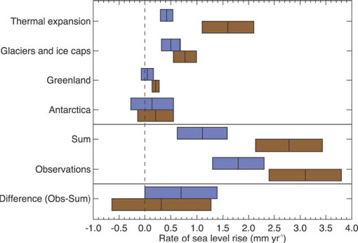
FIGURE 1.6 IPCC (2007) estimates of the primary contributions to global mean sea-level change for 1961 to 2003 (blue) and for 1993 to 2003 (brown), compared to the observed rate of global sea-level rise from tide gages and satellite altimetry. The bars represent the 90 percent error range. The relative contributions of these components has changed in recent years, as discussed in this report. SOURCE: Figure 5.21 from Bindoff et al. (2007).
Finally, the large mass of glaciers and ice sheets exerts an additional gravitational pull that draws ocean water closer. As the ice melts, the gravitational pull decreases, ice melt is transferred to the ocean, and the land and ocean basins deform in response to the loss of land ice mass. These gravitational and deformational effects create regional patterns of sea-level change. Modern melting of ice masses that are nearby (Alaska glaciers) or large (Greenland and Antarctic ice sheets) has the largest effect on sea level in the northeast Pacific Ocean, reducing the land ice contribution to local sea-level rise on the order of tens of percent. The influx of fresh melt water to the ocean also decreases seawater salinity and thus density near shore, which further contributes to regional sea-level variations.
Changes in Land Levels
Regional and local land motion along the U.S. west coast is caused by the ongoing response of the solid earth to a massive loss of ice at the end of the last ice age, tectonics, compaction of sediments, and the removal or addition of fluids from underground reservoirs. During the last glacial maximum, the weight of the ice depressed the land under the ice mass. As the ice melted, the land beneath rose at rates up to 50–100 mm yr-1 (e.g., Shaw et al., 2002), and the ocean floor subsided as ice melt was added to the ocean basins, exerting a considerable load (on the order of 100 t m-2 for a sea-level rise of 100 m; Figure 1.7). These isostatic adjustments produced a characteristic pattern of sea-level change, with land uplift and relative sea-level fall near the major ice centers, and relative sea-level rise everywhere else. Box 1.2 illustrates the effect of glacial isostatic adjustment on relative sea level along the west coast of the United States over the past 18,000 years.
The west coast of the United States is tectonically active, straddling three plate boundaries: the North American and Pacific plates, which slide past one another along the San Andreas Fault Zone in California, and the Juan de Fuca plate, which subducts under the North American plate along the Cascadia
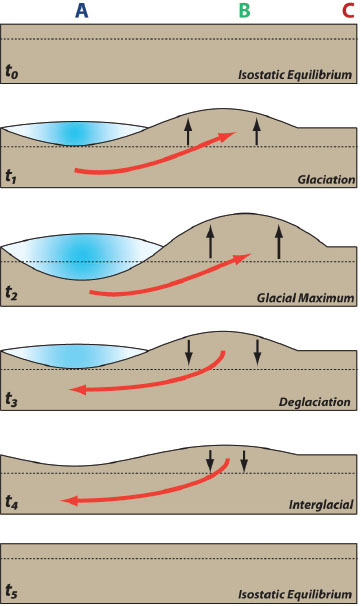
FIGURE 1.7 Response of the solid earth (brown) to the growth and melting of an ice sheet (blue) at increasing distances from the ice (A, B, and C). The addition of an ice sheet causes the land below it to subside and pushes (red arrow) a peripheral bulge outward. With deglaciation, the subsurface material flows back toward the area formerly covered by ice until equilibrium is again reached. SOURCE: Modified from Kemp et al. (2011).
Subduction Zone offshore Washington, Oregon, and northernmost California (Figure 1.8). In subduction zones, strain builds within the fault zone, causing the land to rise slowly before subsiding abruptly during a great (magnitude greater than 8) earthquake. The last great earthquake in the region occurred in 1700, causing a sudden rise in relative sea level of up to 2 m due to subsidence (Atwater et al., 2005). Since that event, much of the coastline of northern California, Oregon, and Washington has been slowly rising. Land motions along the San Andreas Fault Zone have less impact on sea level because the primary motions are horizontal and much of the fault is further inland.
Land subsidence resulting from sediment compaction and fluid (water, petroleum) withdrawal may cause relative sea level to rise. Compaction is particularly important in deltas and other coastal wetlands, where sediments have high water contents. Withdrawal of groundwater and petroleum increases the effective stresses in the surrounding sediments, resulting in consolidation and subsidence, which may be partially reversed by returning fluids to the subsurface.
GEOGRAPHIC VARIATION ALONG THE U.S. WEST COAST
How much coastal inundation can be expected with sea-level rise depends on the local geomorphology, which varies significantly along the west coast of the United States. The geomorphologic features along the coast are primarily the result of a collision between the North American and Pacific plates that began more than 100 million years ago and created steep coastal mountains, uplifted marine terraces, and sea cliffs. Over time, coastal lowlands developed, dominated by long sandy beaches, estuaries, and other wetlands. Most of the California coastline (72 percent or about 1,265 km) is characterized by steep, actively eroding sea cliffs, including about 1,040 km of relatively low-relief cliffs and bluffs, typically eroded into uplifted marine terraces (Figure 1.9), and 225 km of high-relief cliffs and coastal mountains (Figure 1.10). The remaining 28 percent of the coastline is relatively flat and comprises wide beaches, sand dunes, bays, estuaries, lagoons, and wetlands.
The coast of Oregon is dominated by resistant volcanic headlands separated by areas of lower relief. The latter are characterized by uplifted marine terraces, valleys where rivers emerge at the shoreline, and associated estuaries, sand spits, beaches, and dunes. The most extensive sand spits occur along the northern Oregon coastline. The longest continuous beach extends about 96 km, from Coos Bay to Heceta Head, near Florence. The largest coastal dune complex in the United States backs this region (Figure 1.11). Many of the estuarine wetlands have been diked, primarily to provide pasturelands.
BOX 1.2
Changes in Relative Sea Level Along the U.S. West Coast Since the Last Glacial Maximum
During the last ice age, northern Washington was covered by the Laurentide Ice Sheet. When the ice sheet retreated, coastal areas that had been depressed under the weight of the ice sheet were flooded. Relative sea level peaked in that area about 17,000 years ago, reaching values of about 90 m above present in Anacotes (#1 in the Figure) and about 40 m above present in Seattle (#2). Subsequent glacio-isostatic uplift caused relative sea level to fall to its lowest levels about 12,000 years ago (about -40 m in Anacortes and -55 m in Seattle). Relative sea level then rose as ice meltwater was transferred to the oceans and the Laurentide Ice Sheet peripheral bulge began to collapse, causing coastal subsidence.
Glacio-isostatic contributions were much lower in southern Washington, Oregon, and northern California (#3–#9 in the Figure) than for northern Washington, but they were still a dominant influence on sea level. In this area, rates of relative sea-level rise slowed as the effects of glacio-isostatic subsidence decreased. In Eureka, California (#7), for example, relative sea level rose at an average rate of about 7.5 mm yr-1 between 10,000 and 6,000 years before present, then rose at a decreasing rate.
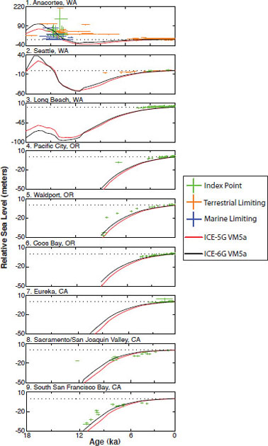
FIGURE Reconstruction of changes in relative sea level over the past 18,000 years for nine locations in Washington, Oregon, and California. Green crosses (index points) represent former sea levels inferred from dated organic sediment in salt and fresh water marshes. Limiting data are from marine shells (blue crosses) and terrestrial peat (orange crosses) that must have been laid down below and above mean sea level, respectively. Red and black lines are model predictions (Peltier and Drummond, 2008; Argus and Peltier, 2010; Peltier, 2010). SOURCE: Data provided by Richard Peltier, University of Toronto.
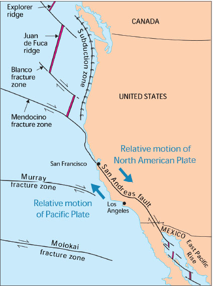
FIGURE 1.8 Major tectonic features along the western United States. Subduction of the oceanic Juan de Fuca and Gorda plates beneath the North American Plate occurs along the Cascadia Subduction Zone, which extends more than 1,000 km from Mendocino, California, to Vancouver Island. South of Cape Mendocino, the North American and Pacific plates slide past one another along the San Andreas Fault Zone. The land west of the San Andreas Fault, from San Diego to Cape Mendocino, is moving northwest relative to the rest of North America. SOURCE: U.S. Geological Survey, <http://pubs.usgs.gov/gip/dynamic/understanding.html>.
The shoreline of southern Washington is dominated by depositional landforms. Beaches, mostly backed by dunes, some developed, extend northward about 100 km from the mouth of the Columbia River to the mountainous Olympic Peninsula (Figure 1.12). The Long Beach Peninsula near the Columbia River and Grays Harbor include some of the most extensive wetlands in Washington, outside of Puget Sound. Some of these wetlands are being restored (e.g., Figure 1.13). Small coastal developments are present on portions of the peninsula and on the low-lying coastal areas to the north.
This report evaluates changes in sea level in the global oceans and along the coasts of California, Oregon, and Washington for 2030, 2050, and 2100. Chapter 2 describes methods for measuring sea level and presents recent estimates of global sea-level rise. Chapter 3 updates the IPCC (2007) estimates of the major components of global sea-level change— thermal expansion of ocean water, melting of glaciers and ice sheets, and transfers of water between land reservoirs and the oceans. Chapter 4 assesses the factors that influence sea-level change along the U.S. west
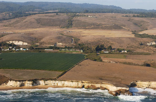
FIGURE 1.9 Uplifted marine terraces, Santa Cruz County, California. SOURCE: Copyright 2002–2012 Kenneth & Gabrielle Adelman, California Coastal Records Project, <www.Californiacoastline.org>.
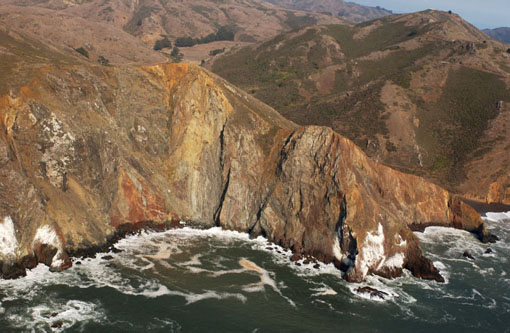
FIGURE 1.10 Steep rocky cliffs of the Marin Headlands north of San Francisco, California. SOURCE: Copyright 2002–2012 Kenneth & Gabrielle Adelman, California Coastal Records Project, <www.Californiacoastline.org>
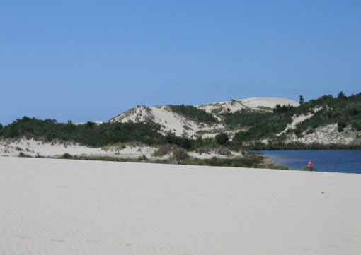
FIGURE 1.11 Oregon Dunes National Recreation Area. The largest coastal dune field in the United States has developed along the central Oregon coast and extends inland up to 3 km. SOURCE: Gary Griggs, University of California, Santa Cruz.
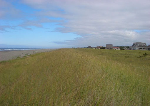
FIGURE 1.12 Long Beach Peninsula, Washington. Sandy beaches backed by dunes dominate the southern coast of Washington. SOURCE: Courtesy of Phoebe Zarnetske, Oregon State University.
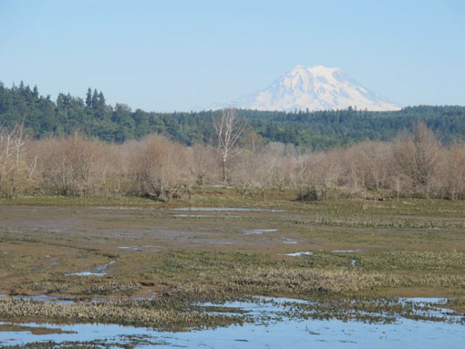
FIGURE 1.13 Tidal wetlands along the mouth of the Nisqually River, Washington, are being restored following removal of a dike built a century ago to drain the area for cattle ranching. SOURCE: Courtesy of Carl Safina; photo taken for the PBS television series Saving the Ocean.
coast, including regional changes in ocean circulation, climate-induced changes in storms, gravitational and deformational effects of land ice change, and vertical land motions. It also summarizes the results of the committee’s analysis of tide gage and GPS records from the California, Oregon, and Washington coasts, which is discussed in detail in Appendix A. Sea-level data from the northeast Pacific Ocean is presented in Appendix B. Data and uncertainties associated with the analysis of gravitational and deformational effects of land ice change are given in Appendix C. The tide gage and vertical land motion analyses draw on leveling data, and a description of leveling data compiled and analyzed for California by James Foster, University of Hawaii, appears in Appendix D. Chapter 5 summarizes recent projections of global and regional sea-level rise and presents the committee’s projections for 2030, 2050, and 2100. The method used to project the cryospheric component of global sea-level rise is described in Appendix E. Chapter 5 also describes what rare, extreme events, such as a great earthquake along the Cascadia Subduction Zone, might mean for local sea-level rise. Chapter 6 summarizes the literature on natural shoreline responses to and protection from sea-level change. Biographical sketches of committee members are given in Appendix F, and a list of acronyms and abbreviations appears in Appendix G.


