Page 303
10
Ozone Air-Quality Models
Introduction
To predict compliance with the ozone air-quality standard at some future date it is necessary to know how ozone concentrations change in response to prescribed changes in source emissions of precursor species: the oxides of nitrogen (NOx) and volatile organic compounds (VOCs). This assessment requires an air-quality model, which in the case of ozone prediction is often called a photochemical air-quality model. The model in effect determines the emission reductions needed to achieve the desired air-quality standard, such as the National Ambient Air Quality Standard (NAAQS) for ozone.
Air-quality models are mathematical descriptions of the atmospheric transport, diffusion, and chemical reactions of pollutants. They operate on sets of input data that characterize the emissions, topography, and meteorology of a region and produce outputs that describe that region's air quality. Mathematical models for photochemical air pollution were first developed in the early 1970s and have been developed, applied, and evaluated since that time. Much of the field's history is described in reviews by Tesche (1983), Seinfeld (1988), and Roth et al. (1989).
The air-quality model is theoretically the ultimate integrator of one's knowledge of the chemistry and physics of the ozone-precursor system. Photochemical air-quality models can be used to demonstrate NAAQS attainment or to educate planners about the emissions controls needed to head toward attainment. Whether or not they are actually used in determining abatement
Page 304
strategies, models are essential for examining of the complex interactions among emissions, meteorology, and atmospheric chemistry.
A practical model consists of four structural levels:
• The conceptual formulation; that is, a set of assumptions and approximations that reduce the actual physical problem to an idealized one, which, within the limits of present understanding, retains the most important features of the actual problem.
• The basic mathematical relations and auxiliary conditions that describe the idealized physical system.
• The computational schemes (numerical procedures) used to solve the basic equations.
• The computer program or code that actually performs the calculations.
The term ''model'' has been used to apply collectively or separately to all four levels. Models of a particular process, or a group of interacting processes, are called component models or modules. The basis for air-quality models is the atmospheric diffusion equation, which expresses the conservation of mass of each pollutant in a turbulent fluid in which chemical reactions occur (Seinfeld, 1986).
For at least a decade, the Environmental Protection Agency (EPA) has offered guidelines on the selection of air-quality modeling techniques for use in State Implementation Plan (SIP) revisions, new source reviews, and studies -aimed at the prevention of significant deterioration of air quality. EPA guidelines (EPA, 1986b) identify two kinds of photochemical model: The urban airshed model (UAM) is the recommended model for modeling ozone over urban areas and EKMA (empirical kinetic modeling approach) is identified as an acceptable approach.
As noted in Chapter 3, the 1990 Clean Air Act Amendments specify that three-dimensional, or grid-based, air-quality models, such as UAM, be used in SIPs for ozone nonattainment areas designated as extreme, severe, serious, or multistate moderate (EPA, 1991b). Grid-based models use a fixed Cartesian reference system within which to describe atmospheric dynamics (Seinfeld, 1988). The region to be modeled is bounded on the bottom by the ground, on the top by the inversion base or some other height that characterizes the maximum extent of vertical mixing, and on the sides by east-west and north-south boundaries, unless the coordinates are rotated. This space is then subdivided into a three-dimensional array of grid cells. The horizontal dimensions of each cell are usually a few kilometers for urban applications. Some older grid-based models assumed only a single, well-mixed vertical cell extending from the ground to the inversion base; current models subdivide the re-
Page 305
gion into layers. Vertical dimensions can vary, depending on the number of vertical layers and the vertical extent of the region being modeled. A compromise generally must be reached between the better vertical resolution afforded by the use of more vertical layers and the associated increase in computing time. Although aerometric data, such as the vertical temperature profile, that are needed to define the vertical structure of the airshed are generally lacking, it is important to use enough vertical layers so that NOx emissions from tall stacks are not overdiluted computationally. There are practical and theoretical limits to the minimum horizontal grid cell size. Increasing the number of cells increases computing and data acquisition effort and costs. In addition, the choice of the dimension of a grid cell implies that the input data—information about winds, turbulence, and emissions, for example—are resolved to that scale. In practice, most urban models use horizontal grid cell of a few kilometers, whereas regional models use horizontal grid cells of tens of kilometers.
There is a need for a set of directives about how to specify the size of the modeling domain, the horizontal grid spacing. to be used, the vertical extent of the modeling region, and the number and resolution of vertical layers. These directives must be based on the exercise of models having a wide range of spatial resolutions and on the comparison of model performance against a wide variety of high-quality field data. It has been found that increasing the horizontal grid spacing in a photochemical air-quality model will generally result in a reduction in the peak ozone concentration. It also is important to provide adequate vertical resolution—the order of five vertical layers or more for urban-scale applications (EPA, 1991b). The minimum amount of meteorological and air-quality data must be prescribed as modeling inputs. The choice of the size of the modeling domain will depend on the resolution available in the data, including the distribution of emissions in the region, the weather conditions, and, to some extent, the computational resources available. The spatial resolution of the concentrations predicted by a grid-based model corresponds to the size of the grid cell. Thus, effects that have spatial scales smaller than those of the grid cell cannot be resolved. Such effects include the depletion of ozone by reaction with nitric oxide (NO) near strong sources of NOx like roadways and power plants.
Several grid-based photochemical air-quality models have been developed to simulate ozone production in urban areas or in larger regions. They differ primarily in their treatment of atmospheric processes and in the numerical procedures used to solve the governing system of equations. Table 10-1 lists grid-based photochemical air-quality models in current use or under development. As noted in Chapter 3, photochemical air-quality models are used in determining the emissions controls needed to attain the ozone NAAQS. But
Page 306
| TABLE 10-1 | |||
| Model | Developer | Status | Reference |
| UAM (Urban Airshed Model | Systems Applications, Inc. | Wide use Documented | Reynolds et al. (1973, 1989 |
| Carbon Bond-II Chemistry | Reynolds (1977) | ||
| Ames et al. (1985) | |||
| UAM | Systems Applications, Inc. | Limited | |
| Carbon Bond-IV Chemistry | |||
| UAM | Radian Corporation | In testing | Tesche et la. (1988a,b) |
| Carbon Bond-IV Chemistry | Code available | Tesche and McNally (1989) | |
| CIT (California Institute of Technology) | California Institute of Technology and Carnegie Mellon | Research applications | McRae et al. (1982) |
| CIT Chemistry | University | Not documented | McRae and Seinfeld (1983) |
| Russell and Cass (1986) | |||
| CIT | Carnegie Mellon | Limited use | |
| SAPRC (Statewide Air Pollution Research Center) Chemistry | University | ||
(Table continued on next page)
Page 307
(Table continued from previous page)
| Model | Developer | Status | Reference |
| CALGRID | Sigma Research | In review | Yamartino et al. (1989) |
| SAPRC Chemistry | Documented | ||
| ROM | EPA | Operational (code and documentation due in 1990) | Lamb (1983) |
| Carbon Bond-IV Chemistry | |||
| RADM (Regional Acid Deposition Model) | National Center for Atmospheric Research and SUNY Albany | Operational | Chang et al. (1987) |
| ADOM (Acid Deposition and Oxidant Model) | ENSR and Ontario | Operational | Venkatram et al. (1988) |
| Ministry and Environment |
Page 308
first, the validity of the model must be demonstrated by its ability to simulate adequately a base-year episode of high concentrations of ozone. Then, using the same meteorology as in the base-year episode, the emissions are hypothetically reduced to the point at which the peak 1-hr ozone concentration in the region does not exceed 120 ppb.
The remainder of this chapter is structured as follows. First the development of meteorological inputs to air-quality models is discussed, followed by a brief discussion of boundary and initial conditions. We then address how attainment of the ozone NAAQS is demonstrated using a grid-based modeling approach. Because urban grid-based photochemical air-quality models have received a great deal of attention in the literature (see, for example, Seinfeld, 1988), we do not devote significant coverage to them here. However, regional air-quality models, which are quite similar in structure to the earlier models used in urban applications, have not undergone the same degree of evaluation and application as their urban counterparts. For this reason, and because such regional models are currently being used to assess ozone abatement strategies in areas like the northeastern United States, we will review regional grid models in this chapter. The particular model on which we focus is EPA's Regional Oxidant Model (ROM). After the analysis of regional models, the general issue of evaluation of model performance is addressed.
Meteorological Input To Air-Quality Models
Grid-based air-quality models require, as input, the three-dimensional wind field for the episode being simulated. This input is supplied by a so-called meteorological module. Meteorological modules for constructing wind fields for air-quality models fall into one of four categories (Tesche, 1987; Kessler, 1988):
• Objective analysis procedures that interpolate observed surface and aloft wind speed and direction data throughout the modeling domain.
• Diagnostic methods in which the mass continuity equation is solved to determine the wind field.
• Dynamic, or prognostic, methods based on numerical solution of the governing equations for mass, momentum, energy, and moisture conservation along with the thermodynamic state equations on a three-dimensional, finite-difference mesh.
• Hybrid methods that embody elements from both diagnostic and prognostic approaches.
Page 309
Objective analysis procedures are inexpensive and simple to use. Their disadvantage is that they contain no physics-based calculations, and the results are highly dependent on the temporal and spatial resolution of the observed wind speeds and directions. Results are often unsatisfactory in areas of the modeling domain where observations are either sparse or not representative of the physical geography. Areas of complex terrain, variations in land use, and ocean-land contrasts cannot be accounted for. Diagnostic procedures impose mass consistency on the flow field through appropriate equations, and can crudely include terrain blocking effects or estimates of upslope and down-slope flows if observed values are entered into the analysis. Diagnostic procedures have modest computational requirements and can require fewer observations than does objective analysis to produce a three-dimensional wind field. Without representative data, however, diagnostic models cannot simulate such features as sea and land breezes. Prognostic numerical prediction models are intended to simulate all relevant physical processes without requiring a significant amount of observed data. These models require specification of the large-scale flow, surface conditions, and the initial state of the atmosphere. Because prognostic models simulate the temperature field in addition to the wind field, it is possible to determine atmospheric stabilities and mixing-height fields from the output. However, the computations performed by prognostic models can be expensive, and they do not necessarily reproduce available observations. Recent developments in data assimilation techniques could overcome the latter problem by forcing models to be more consistent with the available local observations, provided these observations can be shown to be truly representative of the actual meteorological field. Also, with better computer systems becoming available, it is increasingly practical to use full numerical prediction models.
There are several hybrid models that use standard finite-difference techniques for horizontal advection but replace a rigid, vertical, finite-difference grid with one or more layers. The simplest example is a single-layer model in which the height and quantities of potential temperature and moisture, for example, are predicted in the boundary layer (Lavoie, 1972). This hybrid of numerical prediction and layer-averaged approaches is the basis of the EPA Regional Oxidant Model (ROM) (Lamb, 1983). An approach that is becoming more common is the use of the outputs from a prognostic model along with observed data as inputs to a diagnostic model.
An EPA five-city study has identified important limitations in the routinely available meteorological data bases and raises several questions (Scheffe, 1990): Is it possible to set minimum data requirements given the great diversity of the areas in the United States to which air-quality models will be applied? Must data be of sufficient spatial and temporal density to result in
Page 310
such narrow uncertainty bounds that performance evaluation for wind field generation routines is not needed, or is "sufficient data" defined by the amount needed to attain a specified level of uncertainty? An emerging issue in wind field modeling is that of performance evaluation—determining a technical basis for judging the accuracy of simulated wind fields. Current criteria for evaluating wind field modeling performance have not been applied in wind field generation for ozone modeling. Performance evaluation of the meteorological model, independent of the air-quality model, is necessary to ensure that compensating errors are not introduced into predicted ozone concentrations through unjustifiable modifications of the wind field.
There are several important meteorological variables other than wind field. Of particular importance is the treatment of photolysis rates and of the effects on these rates of clouds, urban aerosols, and ozone aloft. Clouds have traditionally been neglected in photochemical grid models because these models have focused on gas-phase pollutants, even though clouds can have a significant effect on the vertical distribution of pollutants (see Chapter 4) and on the attenuation (below cloud) or enhancement (near top of cloud) of photolysis rates. Objective or diagnostic techniques and prognostic modeling also can be used to calculate mixing heights. The key questions relate to the level of accuracy of the spatial and temporal variability in mixing heights. There are no currently accepted procedures for calculating mixing heights, and the mixing-height profile will strongly influence the predicted ozone concentrations in the modeling domain.
Boundary And Initial Conditions
When a grid-based photochemical model is applied to simulate a past pollution episode, it is necessary to specify the concentration fields of all the species computed by the model at the beginning of the simulation. These concentration fields are called the initial conditions. Throughout the simulation it is necessary to specify the species concentrations—called the boundary conditions—in the air entering the three-dimensional geographic domain.
Three general approaches for specifying initial and boundary conditions for urban-scale applications can be identified: Use the output from a regional scale photochemical model; use objective or interpolative techniques with ambient observational data; or, for urban areas sufficiently isolated from significant upwind sources, use default regional background values and expand the area that is modeled and lengthen the simulation period to minimize uncertainties due to a lack of measurements.
In the ideal case, observed data would provide information about the con-
Page 311
centrations at the model's boundaries. In practice, however, few useful data are generally available—a result of the difficulty in making measurements aloft and the fact that monitoring stations tend to be in places where air-quality standards are expected to be violated. An alternative approach is to use regional models to set boundary and initial conditions. This is, in fact, preferred when changes in these conditions are to be forecast. In any event, simulation studies should use boundaries that are far enough from the major source areas of the region that concentrations approaching regional values can be used for the upwind boundary conditions. Boundary conditions at the top of the area that is being modeled should use measurements taken from aloft whenever they are available. Regional background values are often used in lieu of measurements. An emerging technique for specifying boundary conditions is the use of a nested grid, in which concentrations from a larger, coarse grid are used as boundary conditions for a smaller, nested grid with freer resolution. This technique reduces computational requirements compared to those of a single-size, fine-resolution grid.
Simulations of a multiday episode, beginning at night, when concentrations of ozone precursors are the lowest, minimize the influence of initial conditions on ozone concentrations predicted 2 and 3 days hence. Initial conditions are determined mainly with ambient measurements, either from routinely collected data or from special studies. Where spatial coverage with data is sparse, interpolation can be used to distribute the surface ambient measurements. Because few measurements of air-quality data are made aloft, it is generally assumed that species concentrations are initially uniform in the mixed layer and above it. To ensure that the initial conditions do not dominate the performance statistics, model performance should not be assessed until the effects of the initial conditions have been swept out of the grid.
Demonstration of Attainment
Chapter 3 introduced the SIP concept wherein the demonstration of attainment of the ozone NAAQS is based on future-year simulations. These demonstrations require projections of emissions and of initial and boundary conditions. The use of "background" boundary conditions would require an estimate of how these background conditions might change in response to regional changes in emissions. Boundary conditions can be based on future-year regional modeling. Initial conditions are typically reduced in proportion to emission reductions from the base to future year.
A major question is "What is an acceptable procedure for demonstrating attainment?" Previous model applications for control strategy development
Page 312
have, for the most part, avoided complex scientific issues by focusing on one to three worst-case episodes, interpreting model results in a deterministic form without regard to modeling uncertainties and the statistical form of the ozone NAAQS. There is a critical need to identify and investigate methodologies for transforming results from deterministic models into a probabilistic form, so that informed decisions can be made about the efficacy of the selected emissions control strategy in achieving compliance with the ozone NAAQS. Other issues have not been adequately addressed in the context of ozone attainment demonstration. These include the number of episodes that need to be modeled and the duration of each episode.
When the episodes to be modeled have been selected, it must be decided whether attainment should be demonstrated for all modeled episodes. For a particular episode, it is not a simple matter to decide which measure will be used to show attainment. For example, how should bias—under- or over-prediction of the peak ozone concentration—in the base year be addressed? One approach is to ignore any bias in the base year and consider attainment to be achieved if future-year predictions produce peak values below the NAAQS. Alternatively, the future-year peak ozone predictions could be normalized relative to the bias in the base-year simulation; if peak ozone is underpredicted by 10% in the base year, the future-year predicted peak ozone is increased by the same amount. Such questions related to how attainment is demonstrated have not been addressed adequately by the regulatory community.
An aerometric data base is a critical component of a modeling application. Such a data base is needed to provide input to the model and to serve as a tool for assessing model performance. The elements of an aerometric data base for photochemical air-quality modeling are presented in Table 10-2. Most aerometric data bases use routine surface meteorological and air-quality measurements, either no upper-air meteorological data or routine National Weather Service balloon soundings only, and no air-quality data from aloft. A data base with such limitations does not contain enough information to characterize the three-dimensional meteorological and air-quality fields in space and time required for the model. An issue that must be addressed in an attainment demonstration is whether special aerometric measurements should be made over a limited period to provide a more extensive data base than is routinely available or whether a larger number of episodes should be considered with the more routine data base.
Page 313
| Table 10-2 | ||
| Extent of database | ||
| Extensive/Intensive | Routine | |
| Upper air meteorology (wind speed and direction, temperature, relative humidity, pressure) | ||
| Number of soundings per day | 4-8 | None or limited to routine National Weather Service or military installation observations |
| Vertical resolution | 100 meters | None |
| Air quality aloft | ||
| Species | Ozone, NO, NO, speciated VOCs | None |
| Number of profiles per day per site | > 3 | None |
(Table continued on next page)
Page 314
(Table continued from previous page)
| Extent of database | ||
| Extensive/Intensive | Routine | |
| Surface meteorology | ||
| Additional characteristics | Ultraviolet-radiation | |
| Temporal resolution | Continuous and hourly averaged | Continuous and hourly averaged |
| Surface air quality | ||
| Species and temporal resolution | Ozone, NOx, NO (continuous) Speciated VOCs (2-4 times per day) Secondary species (continuous) | Ozone, NOx, NO (hourly averaged) |
Another major issue is what should be done when sufficient air-quality data do not exist to perform a definitive model performance evaluation, but a SIP is still required. For some areas in this category, a grid-based, three-dimensional model simulation is inappropriate. However, because government agencies must make billion-dollar decisions concerning emissions control strategies, they should require that sufficient data be collected to support a proper air-quality model analysis. Use of a model in a data-poor situation, with a large number of default inputs, can delude regulators into believing they have a viable plan when none exists, but model use in a data-poor situation can lead to better analysis in the future. A model can be used as a tool to guide the collection of data and identify the most important data needs for a given region, such as was done in planning the Southern California Air Quality Study (SCAQS) (Lawson, 1990) and the San Joaquin Valley Air Quality Study (SJVAQS)/Atmospheric Utility
Page 315
Signatures, Predictions, and Experiments (AUSPEX) (Ranzieri and Thuillier, 1991).
Regional Grid Models
Grid-based models have been developed to simulate oxidant production and acid deposition over the eastern United States. The grid size of these models ranges from 18.5 to 127 kilometers (km). Only one of them, EPA's ROM, has been used extensively to examine the effects of emission reductions on ozone concentrations in urban, suburban, and rural areas. Development of this model began in 1977, after EPA-sponsored field programs revealed the regional nature of the ozone problem in the northeastern United States. Grid-based models and their evaluation are described here in detail, as these models are relatively new compared to urban models.
In the 1980s, Liu et al. (1984) developed a three-layer regional transport model with a grid size of 80 km that covered the domain of the Sulfate Regional Experiment (SURE) sites. (See Chapter 4.) Winds and mixing heights were obtained by interpolating observations from the National Weather Service radiosonde network, and the model used a version of the carbon bond mechanism (CBM-II). Liu and co-workers evaluated the performance of the model by comparing the time-series of ozone concentrations at the SURE sites for July 16-23, 1978—the most intense episode of high concentrations of ozone that year. The model has been updated to incorporate a nested plume model that treats large point sources; it has been applied, with different grid sizes, to western Europe, to the eastern United States, and to central California (Morris et al., 1988). Performance in the East was evaluated by comparison with ozone data from the SURE sites for Aug. 15 to Sept. 15, 1978. The overall correlation coefficient between the model and observations for all the daylight hourly data was 0.64; the model tended to underpredict the higher ozone concentrations and overpredict the lower ones. The model also overpredicted nighttime concentrations at many sites, possibly because of the poor representation of surface removal by dry deposition.
Two comprehensive models, RADM (regional acid deposition model) and ADOM (acid deposition and oxidant model), have been applied principally to simulations of acid deposition, with only limited evaluation of results for ozone (Middleton et al., 1988; Venkatram et al., 1988). RADM is driven by meteorological input from a mesoscale model (Anthes and Warner, 1978). It uses a lumped chemical mechanism (Stockwell, 1986; Stockwell et al., 1990), and it has a grid size of 80 km and either 6 or 15 vertical layers (Chang et al., 1987). Middleton and Chang (1990) have made comparisons of daily maximum ozone concentrations for three periods, one of which had high ozone concentrations;
Page 316
data from three to six stations were used.
ADOM is driven by meteorological input from the Canadian numerical weather prediction model and a high-resolution boundary layer model. It uses a condensed chemical mechanism adapted from Lurmann et al. (1986b) and has a grid size of 127 km and 12 vertical layers (Venkatram et al., 1988). Karamchandani et al. (1988) made comparisons with ozone time series at four rural stations, and showed ratios of observed to modeled ozone for June 9-17, 1983, for the northeast. Limited emissions reduction scenarios were examined, with results presented only for Ontario (Karamchandani et al., 1988).
The model of McKeen et al. (1991a) is similar in many respects to RADM. It is driven by the same mesoscale model, and it uses a version of the Lurmann et al. (1986b) chemical mechanism. It has a grid size of 60 km and 15 vertical layers and covers the eastern half of the United States. A preliminary evaluation was made for July 4-7, 1986. This period of high ozone concentrations was selected because it coincided with an intensive field measurement program at Scotia, Pennsylvania (Trainer et al., 1987). Model results for ozone (averages for 1:00 p.m. to 5:00 p.m.) were compared to data from the Aerometric Information Retrieval System (AIRS) (EPA, 1987) for the final two days of the simulation, and maps were shown of model results for NOx and isoprene, averaged over 0900-1700 hr, as were average vertical profiles for odd-nitrogen species and various VOCs. The budgets of ozone, NOx, and isoprene, averaged over the model domain, were discussed. Detailed comparisons with the Scotia data are not yet available (M. Trainer, NOAA, pets. comm., Nov. 1991).
The major shortcoming with the studies (Liu et al., 1984; Middleton and Chang, 1990; McKeen et al., 1991a) described above is that the model evaluations focus almost exclusively on surface ozone in rural air, usually for a single pollution episode. This is in part because of the lack of high-quality data for NOx and VOCs in rural locations (see Chapter 7). Only the study by McKeen et al. (1991a) shows model predictions for NOx, and none of the studies shows the spatial concentration fields predicted for any of the anthropogenic VOCs. None of the models has been evaluated systematically by rigorous comparison of predictions for ozone and its precursors for the range of meteorological conditions found in the eastern United States.
The Regional Oxidant Model (ROM) is a grid-based photochemical air-quality model with a grid size of ˜ 18.5 kin, designed to simulate ozone formation and transport over the eastern United States (Figures 10-1 and 10-2). The transport is governed by wind fields interpolated on an hour-by-hour basis from observations at surface and upper air stations. The model includes parameterizations for the effects of cumulus clouds on vertical transport; nighttime wind shear and turbulence episodes associated with the nocturnal jet stream; mesoscale vertical motions induced by the interaction of terrain and the large-scale flow; and the
Page 317
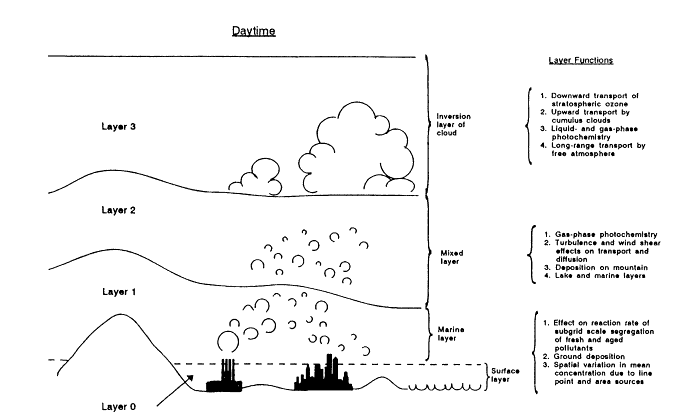
Figure 10-1.
Regional oxidant model (ROM) vertical structure of the atmosphere during daytime conditions. Source: Schere and Wayland, 1989.
Page 318
effects of differences in terrain on advection, diffusion, and deposition. Lamb (1983, 1984) described the theoretical basis and design of ROM. The model incorporates the Carbon Bond 4.0 (CBM-IV) chemical mechanism (Whitten and Gery, 1986). Most studies with ROM2.0 have used the National Acid Precipitation Assessment Program (NAPAP) 1980 emissions inventory (Version 5.3) for anthropogenic species and the inventory of biogenic VOCs described by Novak and Reagan (1986), and have focused on the northeastern United States (Figure 10-2a), although a few studies have been conducted for the Southeast (Figure 10-2b).
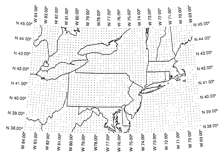
Figure 10-2a
Regional oxidant model (ROM) domain, Northeastern United States. Source: Schere and Wayland, 1989.
The advantage of the physical layered structure of ROM (Figure 10.1) over a finite-difference representation of the vertical is that it allows high horizontal resolution without excessive amounts of computer memory being consumed by many vertical layers. This is particularly important for a model that uses 28 chemical tracers as well as meteorological fields. There are problems with its approach, however, in mountainous regions, such as the Appalachians, Rocky Mountains, or along the West Coast of the United States, where the atmospheric boundary layer has more than one level. Pollutants thus could be emitted in any
Page 319
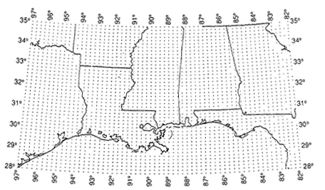
Figure 10-2b
ROM domain, Southeastern United States. Source: Schere and Wayland, 1989.
of the layers shown in Figure 10-1, or even above the model layers, depending on environmental stability and winds. Moreover, the transfer rates between layers are affected by the presence of mountains whose heights are greater than the height of the boundary layer. Multi-atmospheric boundary layers also can form along coastal regions because of sea breeze circulations. In some cases their effects can be characterized in a three-layer atmosphere; in other cases such a simple parameterization will not work. The same holds true for parameterizations of the effects of cumulus transport and wet deposition on transfer rates. There often is not enough information in a three-layer model to diagnose the predominant mode of convection (by ordinary cumulus clouds, by deep convection, or by mesoscale convective systems). The deeper modes of convection require information about the deeper tropospheric structure and its modulation by convection.
A major limitation of ROM is that it is a ''hardwired'' model such that resolution cannot be readily expanded in the vertical direction as better computer resources become available. There has been a revolution in supercomputers and workstations in the decade since ROM was designed. Numerical prediction models with 15 to 30 levels in the vertical direction and 15 km resolution laterally are now being run operationally in the United Kingdom and elsewhere. The
Page 320
output of such models could be used to drive an improved ROM with vertical resolution that matches the larger-scale model grid and uses some of the physical routines, such as the convective parameterization schemes, available in the larger-scale model.
The domain of ROM is relatively small, a consequence of its high spatial resolution. The effect of initial and boundary conditions is therefore of concern. The model is initialized with "clean" tropospheric background conditions—ozone at 35 parts per billion (ppb), NOx at 2 ppb, and nonmethane VOCs at 15 ppb carbon—and it is allowed to run chemically for 10 hr before the actual start of a run. This procedure reduces the value for NOx to ˜0.2 ppb (Schere and Wayland, 1989). ROM takes boundary conditions for ozone to be the average of values (6-hour mean) at three "relatively rural" sites in Ohio, West Virginia, and Virginia; the model is then re-equilibrated for 1.5 hours, starting with the equilibrated initial conditions and the new ozone value, to obtain daytime and nighttime boundary conditions. The equilibrated initial and boundary conditions for NOx are exceedingly (and probably unrealistically) low. The effects of the boundary conditions are expected to be greatest in the west and south of the modeled area, and least in the Northeast corridor, the focus of the model.
ROM2.0 has been evaluated by making comparisons with measurements of ozone, NOx, and nonmethane VOCs collected between July 12 and August 31, 1980 (Schere and Wayland, 1989). The model was run without re-initialization for this six-week period, which was chosen to coincide with three major field programs in the Northeast: the Northeast Regional Oxidant Study (NEROS) (Vaughan, 1985), the Persistent Elevated Pollutant Episode (PEPE) study, and the Northeast Corridor Regional Modeling Program (NECRMP). These programs were designed to provide data for input to and evaluation of regional and urban models applied to the Northeast, and each included a major component of aloft data obtained by aircraft. The frequency of upper air soundings was increased from two to four per day at the stations within the domain of ROM2.0 during intensive NEROS field study periods. The major shortcoming of the data available for this period is the relative dearth of rural data, particularly for NOx. None of the NOx monitors were sensitive to concentrations below 5 ppb, and concentrations below this level are often found at rural sites (see Chapter 7). The ozone data were obtained from EPA's SAROAD data base (now AIRS [EPA, 1987]) supplemented by data for southern Ontario (obtained from Environment Canada and the Ontario Ministry of the Environment). In all, 214 sites were studied, primarily in or near urban areas.
ROM2.0 results for ozone were evaluated (Schere and Wayland, 1989) by examining frequency distributions for groups of measurement sites that had common characteristics as discussed below. This method of comparison was chosen over a point-by-point comparison because of the inherent uncertainty in
Page 321
| TABLE 10-3 | ||||||
| Concentration range, ppb | ||||||
| 5-20 | 5-40 | 40-80 | > 80 | |||
| Group 1, | 0.084 | 0.271 | 0.385 | 0.344 | ||
| 35 sites | (0.043) | (0.063) | (0.045) | (0.056) | ||
| Group 2, | 0.149 | 0.378 | 0.406 | 0.216 | ||
| 39 sites | (0.058) | (0.067) | (0.072) | (0.033) | ||
| Group 3, | 0.159 | 0.438 | 0.466 | 0.096 | ||
| 64 sites | (0.061) | (0.068) | (0.073) | (0.046) | ||
| Group 4, | 0.218 | 0.590 | 0.355 | 0.054 | ||
| 54 sites | (0.063) | (0.060) | (0.043) | (0.040) | ||
| Group 5, | 0.423 | 0.799 | 0.187 | 0.014 | ||
| 20 sites | (0.133 | (0.093) | (0.081) | (0.024) | ||
| Group 6, | 0.044 | 0.262 | 0.627 | 0.111 | ||
| 2 sites | — | — | — | — | ||
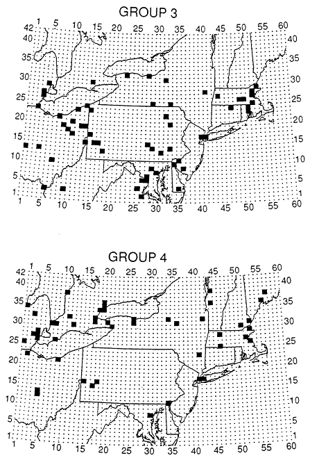
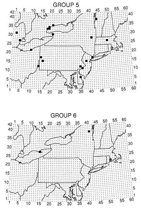
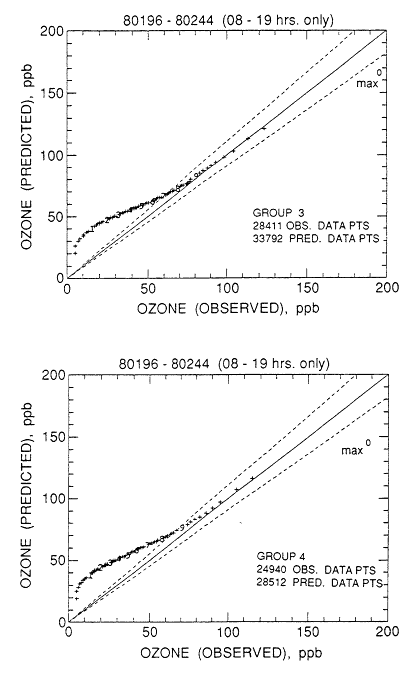
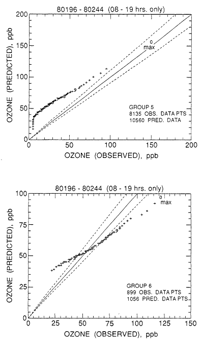
the wind-driven transport component of the model. The sites were divided into groups based on observed frequency distributions, as shown in Table 10-3. Groups 1 and 2 (Figure 10-3) consisted of sites where concentrations above 80 ppb were found most often, and tended to be located along the Northeast corridor. Groups 3 and 4 had lower concentrations of ozone and were distributed throughout the model's domain. Group 5 had many sites where concentrations were below 20 ppb, suggesting contamination by a nearby source of NOx, or problems with the monitor. Group 6, Whiteface Mountain, New York, and Long Point Park in southern Ontario, had few high or low values, characteristic of more remote or mountaintop sites. Comparisons of the frequency distributions for these groups for 8:00 a.m. to 7:00 p.m. LST (local standard time) with model results are shown in Figure 10-4. The figure illustrates the tendency of the model to overpredict ozone at lower concentrations (<50 ppb); some of the
Page 322
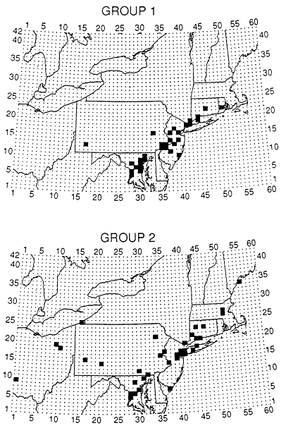
Figure 10-3
ROM grid cell locations (darkened) of monitoring sites within groups
1 through 6 (see Table 10-3). Source: Schere and Way-land, 1989.
Page 323
Page 324
Page 325
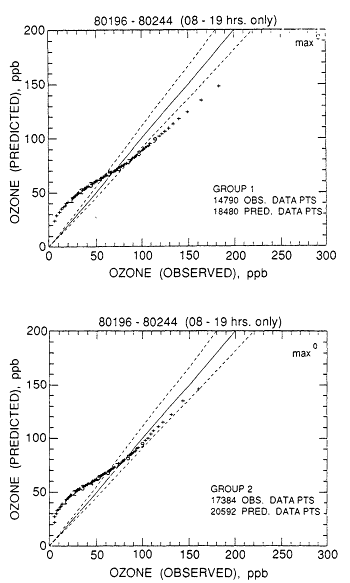
Figure 10-4
Observed versus ROM-predicted cumulative frequency distributions of
daytime (8:00 a.m. to 7:00 p.m., LST) hourly ozone concentrations at each
of six groups of receptor locations over the period from July 14 to
August 31, 1980. Source: Schere and Wayland, 1989.
Page 326
Page 327
Page 328
low values could result from local titration of ozone by NOx at the predominantly urban monitoring sites, an effect that the model would not reproduce. The model underpredicts ozone concentrations above 100 ppb in group 1, which contains the sites where the highest concentrations of ozone are found, but reproduces values from 60 ppb to 120 ppb at sites in groups 3 and 4, most of which lie outside the Northeast corridor. The model also underpredicts concentrations above 75 ppb at the two most remote sites (group 6).
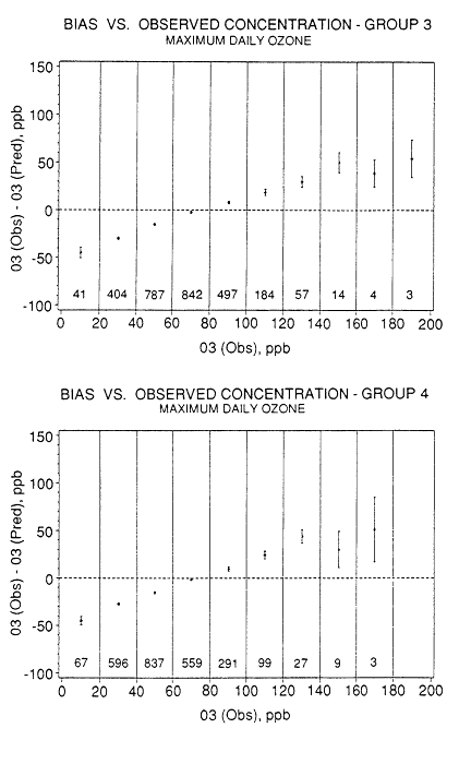
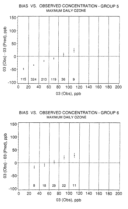
The NAAQS for ozone is based on maximum 1-hour daily concentrations, so these were evaluated separately, using the same groups of stations (Schere and Wayland, 1989). The bias was calculated as the difference between the daily maximum at a site and that in the model (the data were matched in space but not in time on a given day). The bias values are shown in Figure 10-5, as a function of observed ozone, sorted in 20-ppb ranges. The figure shows increasing underprediction of ozone with increasing concentration, and overprediction of low concentrations of ozone. The model performs best for maximum concentrations of 60-100 ppb. The mean underprediction is ˜30 ppb for observed values of 120-140 ppb, and 50-70 ppb for observed values above 160 ppb.
Schere and Wayland (1989) examined the spatial pattern of ozone in the Northeast corridor for five episodes in the six-week period. They compared model results to the pattern of maximum concentrations (the maximum for each station during the episode), as shown in Figure 10-6. The pattern of high concentrations agrees well for July 20-22, less well for July 25-27. The tendency to underpredict the highest concentrations is obvious. Examination of all the episodes shows some characteristic problems. There is often a systematic underprediction of ozone concentrations downwind of Philadelphia, Pennsylvania, such that the urban plume is not apparent in the model results. The urban plumes from Washington, D.C.; Baltimore, Maryland; New York, New York; and Boston, Massachusetts were discernable in the predictions. There appears to be a significant bias in the wind field toward a westerly direction, such that the plumes were carried eastward in the model, whereas the observed data suggest transport to the northeast. Aircraft data show that the model tends to underpredict regional background concentrations of ozone by 20-30 ppb; observations were typically 40-90 ppb whereas the model predicted 40-60 ppb. This could result in part from the low upper boundary value for ozone and in part from underprediction of NOx. The model also underpredicted ozone concentrations aloft in urban plumes.
Model results for NOx were evaluated in the same manner as for ozone, by forming groups of sites. ROM2.0 significantly underpredicts NOx and NO2 (nitrogen dioxide) for urban sites at both the 50th and 90th percentiles of the frequency distributions, as shown in Table 10-4. This could result from the coarse grid of the model or from a systematic underestimate of NOx in the
Page 329
| TABLE 10-4 | ||||
| Daytime, 8:00 a.m. to 7:00 p.m. | All hours | |||
| Percentile | Percentile | |||
| 50th | 90th | 50th | 90th | |
| NOx | 1.8 | 2.3 | 1.9 | 2.5 |
| NO2 | 2.2 | 2.2 | 2.1 | 1.9 |
emissions inventory. Rural measurements of NOx were not available for the evaluation.
Schere and Wayland (1989) evaluated data for VOCs (excluding methane) on a site-by-site basis. The ratios of observed to predicted VOC concentrations for 6:00 to 9:00 a.m. LDT (local daylight time) were typically around 6 for urban areas with a range of 4-10 for specific cities, and somewhat lower, 1.3-8, for data collected after 9:00 a.m. The ratio was lower, about 2, at sites outside large urban areas. The model gave a more accurate prediction of the distribution among the various VOC species than of the total amount. It underpredicted VOCs aloft by a factor of only 1.4 to 2.8, and there were some overpredictions; the more reactive hydrocarbons were underpredicted to a greater extent than were the less reactive ones. VOC emissions appear to be seriously underestimated by the NAPAP 1980 inventory (cf. Chapter 9), and the effect of inaccurate inventories on ROM predictions for ozone requires investigation.
Schere and Wayland (1989) concluded their evaluation of ROM2.0 with the caution that ''a number of issues have arisen that prevent recommending use of the model in a simple unassisted manner for studies of violations of the ozone air-quality standard.'' They stressed that careful analysis of the simulated wind fields and background concentrations of ozone must be made before an episode is used in a model for regulatory application.
Evaluation of Model Performance
Air-quality models are evaluated by comparing their predictions with ambient
Page 330
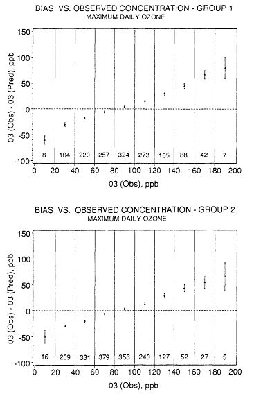
Figure 10-5
Bias versus observed concentration for maximum daily ozone over the
simulation period from July 14 to Aug. 31, 1980, for groups 1 through 6
(see Table 10-3). The 95% confidence interval is shown about the mean
value for each concentration interval. Source: Schere and Wayland, 1989.
Page 331
Page 332
Page 333
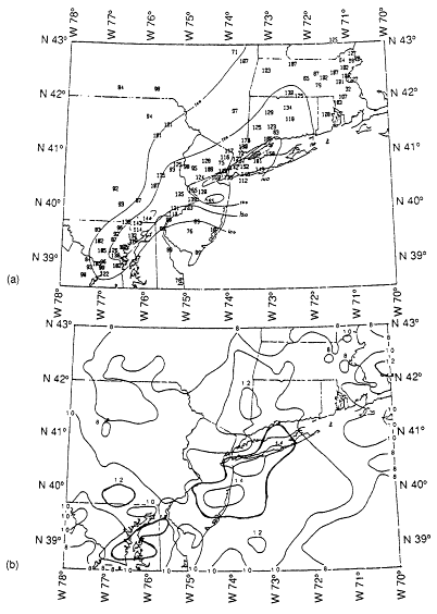
Figure 10-6
Contours of maximum hourly ozone concentrations over the period July
25-27, 1980, for (a) observed and (b) predicted data sets. Contours of
observed data are in concentration units of parts per billion and contours
of predicted data are in units of ppb/100. Source: Schere and Wayland, 1989.
Page 334
observations. Because a model's demonstration of attainment of the ozone NAAQS is based on hypothetical reductions of emissions from a base-year-episode simulation, the accuracy of the base-year simulation is essential. Emissions control prescriptions estimated for an area to meet the NAAQS are sensitive to the base-year model performance. Performance requirements for the base-year simulation are instituted to ensure that the model is adequate to evaluate emissions control strategies. An adequate model should give accurate predictions of current peak ozone concentrations and temporal and spatial ozone patterns. It should also respond accurately to changes in VOC and NOx emissions, to differences in VOC reactivity, to changes in temperature, and to spatial and temporal changes in emissions patterns for future years. Associated with model performance evaluation is the quantification of the uncertainty in predicted emissions control estimates; for example, determination of the relationship between uncertainties in the emissions inventory and uncertainties in model predictions.
A performance evaluation should answer several questions:
• If successfully evaluated for a base case, does the model hold for significantly reduced emissions?
• Does the model correctly reveal the effect of VOC and NOx emissions controls and the influence of chemical reactivity in ozone reduction?
• Has the sensitivity of model performance to variability in input data been established? Have the evaluations been stringent enough to clearly reveal a flawed model?
• What are the component uncertainties in the modeling analysis, and what is the aggregate uncertainty in the control strategy requirement obtained from the model results?
• What is the ability of the model to correctly simulate the effects of individual sources or upwind source regions on local air quality?
• What is the probability that desired air quality will be achieved in the model, given the use of a deterministic model and a limited number of modeling episodes?
The terms "model validation" and "model verification" are frequently used to describe the process of comparing model predictions with observations. These terms can be confusing. If a model is valid, its predictions will agree with the appropriate observations, given a perfect specification of model inputs. A "model performance evaluation'' is the process of comparing a model's predictions with observations. The term "verification" might be reserved to describe a successful, or positive, outcome of the model evaluation process; to determine whether a model is in fact valid.
Traditional photochemical model performance evaluations do not provide
Page 335
enough information to decision makers about the suitability of models for use in regulatory applications (Dennis and Downton, 1984; Seinfeld, 1988). Because evaluation methods have traditionally focused only on the degree to which predictions and observations agree, they are not specifically designed to reveal flaws in a model, in its data base, or in the procedures used to exercise the model. Instead, they are aimed at quantifying the correspondence between predicted and observed ground-level concentrations of pollutants, generally ozone. Although current operational evaluation procedures can indicate how well a model performs in an overall sense relative to similar applications in the past; little direct information is provided about a model's suitability for predicting the effects of emission reductions.
An important question in performance evaluation is whether specific performance goals are specified, or whether minimum criteria for rejection of the results should be set. This is a subtle issue. Key model inputs needed to simulate past episodes have important areas of uncertainty. These inputs include boundary and initial conditions, both on the ground and in the air, and emissions. Sometimes the uncertainties in these inputs are large enough that the temporal and spatial features of ozone behavior can be reproduced reasonably well by variation of the inputs within their ranges of uncertainty. At other times, such variation does not produce adequate agreement between predictions and observations.
Figure 10-7 shows an ozone time series for a UAM simulation of an episode of high concentration of ozone on Sept. 16-17, 1984, in the South Central Coast air basin of California. The solid line represents the hourly base-case model predictions for the Simi monitoring station. The boxes indicate the ozone concentrations observed for each hour. The vertical lines represent the estimated overall uncertainty and representativeness of the spatial distribution of ozone measurements. The thin solid lines enclose an ensemble of time series profiles obtained from more than a dozen model runs focusing on uncertainties in the predicted mixing heights. These uncertainties were derived from a numerical mixed-layer model (Tesche et al., 1988c). Ideally, the ensemble of ozone predictions (enclosed by the thin solid lines) would trace a path within the upper and lower uncertainty bounds of the hourly ozone measurements. If this were the case, the predictions would match the observations within experimental uncertainty. This is not the ease in the example presented here; the model underestimates the peak ozone concentration, and the variability in afternoon ozone predictions that results from mixing-height uncertainties appears to be comparable to the estimated uncertainty in the ozone measurements.
Model performance evaluation procedures and tests must be designed to reveal flaws in assumed input information and model components in order to ensure that a model is producing the right answer for the right reason. In the past, ozone-modeling protocols accepted photochemical model results as ade-
Page 336
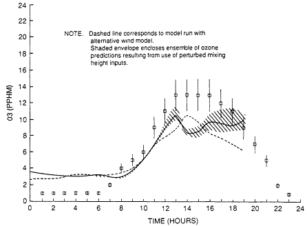
Figure 10-7
Ozone predictions and observations; Sept. 17, 1984
Simi monitoring station. Source: Tesche et al., 1990.
quate if the bias and error statistics were comparable to those of previous, similar studies, but little attention was given to whether the previous simulations adequately met policy-making needs.
The performance of photochemical models, judged by commonly reported statistical procedures, appears to have reached a plateau (Seinfeld, 1988). Current grid-based photochemical models reproduce hourly averaged ozone concentrations to within 30-35% of measured values, and the peak 1-hr concentration is often reproduced to within 15-20%. Tesche (1988) has compiled most of the ozone simulations reported prior to 1988, and the results are summarized in Figure 10-8. The statistics on which Figure 10-8 is based are pairs of hourly averaged predictions and observations at the various monitoring stations in each region. Sixty-seven percent of the single-day simulations exhibit underestimation of ozone, and 62% of the multiday simulations show underestimation of ozone concentrations. This performance is consistent with an underestimation of VOC emissions.
Despite more than a decade of accumulated experience in photochemical model evaluation and refinement, there has been no focused attempt by regu-
Page 337
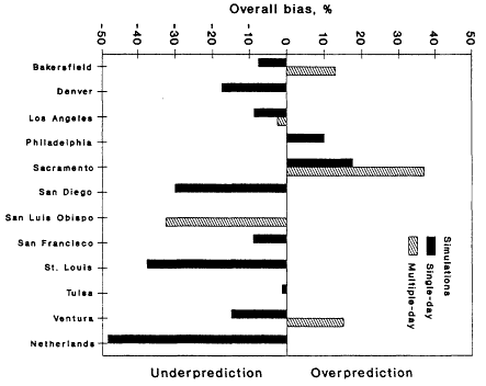
Figure 10-8
Overall bias in hourly averaged ozone predictions by urban area for single- and
multiple-day simulations of episodes of high concentrations of ozone for model
applications prior to 1988. Source: Tesche, 1988.
latory agencies, model developers, or others to derive a consistent set of evaluation procedures from among the techniques in common use—notwithstanding the widely recognized need for such methodology.
Model Performance Evaluation Procedures
Before a photochemical model is applied to simulate the effects of emissions controls, the model must be shown to reproduce the chemical and physical processes that govern ozone formation. This kind of assessment, referred to as model performance evaluation, involves the compilation of emissions, meteorological, air quality, and chemical data drawn from an actual episode. This
Page 338
information is used in the exercise of the model. Through various statistical and graphic means, the model predictions and air-quality observations are compared to determine the fidelity of the simulation.
Specific numerical and graphic procedures have been recommended for evaluation of the performance of grid-based photochemical models (Tesche et al., 1990). The methods suggested include the calculation of peak prediction accuracy; various statistics based on concentration residuals; and time series of predicted and observed hourly concentrations. Four numerical measures appear to be most helpful in making an initial assessment of the adequacy of a photochemical simulation (Tesche et al., 1990):
• The paired peak prediction accuracy.
• The unpaired peak prediction accuracy.
• The mean normalized bias.
• The mean absolute normalized gross error.
Graphic procedures are suggested to complement the statistical approaches. Finally, a minimum set of six diagnostic simulations is recommended as part of performance evaluations.
Diagnostic Evaluation Procedures of Model Performance
The diagnostic evaluation procedures for models discussed in this section are used to determine the causes of failure of a flawed model; to stress a model to ensure failure if the model is flawed; and to provide additional insight into model performance beyond that supplied through the operational evaluation procedures previously discussed. Frequently, operational model evaluation does not convey enough information about the model and data base to allow their use in emissions control strategy development and testing. Particularly in complex air basins, such as the South Coast air basin of California, the model evaluation process should be supplemented with additional diagnostic analyses that probe further into the comparisons between prediction and observation, attempting to ensure that the ozone response given by the model is correct. This section discusses a series of tests and comparisons that are useful in diagnostic analysis of photochemical models. The general categories of these analyses are: diagnostic simulations, testing of species other than ozone (when adequate data permit), examination of model-predicted fluxes and pollutant budgets, and sensitivity-uncertainty testing. In some cases the tests must be supported by high-quality aerometric data bases, only now available in some areas due to the high cost of their acquisition.
Page 339
Five diagnostic simulations are suggested to accompany the numerical and graphic comparisons of predictions and observations (Tesche et al., 1990): zero emissions, zero initial conditions, zero boundary conditions, zero surface deposition, and mixing-height variations.
Zero Emissions
The purpose of the zero-emissions simulation is to ensure that the base-case simulation results are influenced appropriately by the emissions inputs or, conversely, are not over-influenced by initial and boundary conditions. Removing all emissions should lead to much lower concentrations of reactive species. The zero-emissions simulation is performed by running the base-case scenario with all emission values reduced to zero. All other model input files remain unchanged from the base case.
The diagnostic run should produce significantly reduced concentrations—close to background or to the concentrations representing the inflow boundary conditions. If not, there is reason to question the accuracy of the simulation. Lack of sensitivity to emissions can indicate inappropriately high initial conditions, improper boundary conditions, or some flaw in the model itself. Quite apart from these concerns, insensitivity to emissions raises serious questions about the usefulness of the simulated episode for control strategy development and assessment.
Zero Initial Conditions
The zero-initial-conditions simulation reveals how many of the predictions from the second (or third) day result from the initial field used to start the base-case simulation. This test simulation is performed by setting all initial concentrations as close to zero as possible, while avoiding numerical instabilities. Deficit enhancement and time series graphs can be used to display the results of this simulation. If the effect of the initial field is completely gone by the second or third day, the deficit enhancement graphs will indicate essentially no differences between the diagnostic and base-case runs on the following days. For stagnation episodes, some residual effects of initial conditions could be seen even on the third day of a multiday simulation (Tesche and McNally, 1989).
Zero Boundary Conditions
The zero-boundary-condition simulation examines the influence of boundary
Page 340
values on second (or third) day concentrations, particularly in regions where the base-case predictions are highest. This simulation helps identify situations in which the base-case results are greatly affected by the boundary conditions. The simulation is performed by setting all inflow and outflow boundary values to zero, including those for the top surface of the modeling region.
Zero Surface Deposition
The zero-surface-deposition simulation addresses the influence of dry surface deposition removal on concentrations of primary and secondary species. The diagnostic run is performed by setting deposition velocities for all species to zero in the base-case simulation. Although deposition tests have not been reported in previous model evaluation studies, some general guidelines can be suggested. For primary species, such as NOx and VOCs, when deposition is neglected the downwind concentration fields should increase relative to the base case in a manner consistent with the deposition velocities for each primary species. For secondary species, such as ozone, the effect of a change in the deposition of primary species will depend on how that change propagates through the nonlinear chemistry.
Mixing-Height Variations
Mixing heights have a direct and often significant influence on ozone concentrations. The objective of the mixing-height diagnostic simulation is to reveal the degree to which ozone concentrations are influenced by the height of the mixed layer. At a minimum, one diagnostic run is suggested in which the hourly mixing-height values are uniformly increased by 50% above the base-case account. This increase is somewhat larger than the expected uncertainty in estimates of mixing heights typically encountered. Therefore, this simulation should provide a bound on the change in ozone predictions resulting from uncertainties in this input. Increased mixing heights typically reduce ozone concentrations, although the reduction is usually less than a one-to-one change. This effect can be seen by moving toward the origin along a line of constant VOC/NOx ratio on an ozone isopleth plot (see Chapter 6). One might choose, instead, to reduce the hourly mixing heights by 50%. The resultant changes in ozone concentrations under this scenario will typically be comparable in magnitude but of opposite sign to those for the mixing height increase.
Page 341
Dependence on Initial and Boundary Conditions
Given the dependence of model results on initial and boundary conditions, it is of interest to quantify that dependence. Russell et al. (1989) performed a series of diagnostic simulations to identify how grid-based airshed model predictions change with changes in boundary and initial conditions. Initial conditions alone (in a simulation without emissions) led to the development of an air mass with elevated concentrations of ozone and VOCs that would last for several days before being slowly depleted by ground-level deposition and atmospheric chemistry. Predictions on the first and second day of a three-day simulation were dependent on initial conditions of VOC and NOx. By the third day, most of the initial-condition-dominated air mass had left the modeling region, although part of the region was still influenced. Boundary conditions primarily influence the regions near the boundary, with a small influence in the central modeling region. Reducing both boundary and initial conditions to background concentrations led to less than a 4% reduction in peak ozone and exposure predictions from the base-case simulation that used more representative values.
However, if emissions are reduced by 50% or more, the role of initial and boundary conditions increases and cam become significant. For example, diagnostic simulations show that there are enough VOCs in the boundary conditions to form significant amounts of ozone when there are no VOC emissions from any source. Trajectory model studies show similar findings, and this is particularly important because trajectory model simulations are usually for less than 1 day. Simulations of less than 1 day are very sensitive to the choice of initial and upper level boundary conditions. Studies of boundary and initial condition effects suggest that large modeling domains and multiday (preferably, 3 or more) simulations are necessary for testing the effects of control strategies, and it is preferable to have model domain boundaries in relatively clean, rural regions.
Assessing Simulation Results
Decision makers and regulatory agencies seek quantitative performance standards by which to judge new models as acceptable. Each photochemical modeling episode exhibits distinctive aerometric and emissions features. Each model's available data base also is unique in the amount and quality of observations available to support model evaluation and testing. In addition, the particular set of modeling procedures and codes makes each application distinctive. Therefore, automatic use of standards for acceptance or rejection raises the risk of accepting a model evaluation that gives seemingly ''good" performance statistics but for
Page 342
the wrong or misleading reasons. It also could lead to rejection of a model evaluation that violates criteria for reasons related to input inaccuracies rather than to fundamental flaws.
Instead of prescribing fixed performance standards, Tesche et al. (1990) suggest the following approach. From more than 15 years of photochemical model development and testing, photochemical grid model simulations generally produce peak (unpaired) prediction accuracy, overall bias, and gross error statistics in the approximate ranges of 15-20%, 5-15%, and 30-35%, respectively (Figure 10.8). A study that follows an approved ozone-modeling protocol but falls outside all these ranges would not be rejected unless evidence from the model's diagnostic simulations and the other numerical measures and diagnostic tests suggested unusual or aberrant behavior. For model simulations falling within these ranges, some additional diagnostic analyses could be appropriate to lend further support to the contention that the simulation is acceptable. For model results outside the ranges given for any one of these areas, it should be incumbent on the modeler to explain why the performance is poorer than that commonly achieved in similar applications and whether the causes of poorer performance will adversely affect the use of the model in control strategy evaluations. This method provides reviewing agencies with a general model performance target, but still guards against the inappropriate rejection of less accurate model simulations when appropriate explanations can be provided.
Multispecies Comparisons
The development of evaluation procedures that test photochemical model performance for species other than ozone can provide a basis for accepting or rejecting a model (or a model simulation); they significantly improve the chances that a flawed model will be identified. Adequate model performance for several reactive species increases the assurance that correct ozone predictions are not a result of chance or fortuitous cancellation of errors introduced by various assumptions. Multispecies comparisons could be the key in discriminating among alternative modeling approaches that provide similar predictions of ozone concentrations.
To date, most model evaluation studies present results only for ozone (Tesche, 1988), although there are a few limited tabulations of NO2 predictions (Wagner and Ranzieri, 1984). Studies reported by Roth et al. (1983), Tesche (1983), Russell and Cass (1986), Wagner and Croes (1986), and Russell et al. (1988a,b) are among the few that present performance evaluation statistics for associated pollutants. Lack of ambient measurements for such pollutants is the major reason for the limited number of past studies. The data bases for the
Page 343
Southern California Air Quality Study and the San Joaquin Valley Air Quality Study (SJVAQS)/Atmospheric Utility Signatures, Predictions, and Experiments (AUSPEX) now allow for several comparisons with species other than ozone. The SCAQS data in particular afford a level of testing of photochemical models and modules, such as the chemistry mechanism, not previously possible. The availability of ambient air measurements for speciated organics and for key species such as formaldehyde (HCHO), peroxyacetyl nitrate (PAN), nitrogen dioxide (NO2), hydrogen peroxide (H2O2), nitric acid (HNO3), and organic acids will allow not only more extensive operational model testing but also diagnostic and comparative evaluations. Finally, the SCAQS data base, or similar data bases that will be assembled in the future, such as one from the SJVAQS/AUSPEX (Ranzieri and Thuillier, 1991), also offer the potential for evaluations of alternative chemical kinetic mechanisms.
Evaluation of model performance for precursor and intermediate species as well as for product species other than ozone is recommended when ambient concentration data for these species are available. Comparisons of observed and predicted concentrations for all important precursors, intermediates, and products involved in photochemical air pollution—such as individual VOCs, nitric oxide (NO), nitrogen dioxide (NO2), PAN, ozone, H2O2, nitrous acid (HONO), and HNO3—are useful in model evaluation, especially with respect to the chemistry component of the model (Dodge, 1989, 1990). Accurate matching of ozone alone may not be sufficient to indicate that a chemical mechanism is correct. Comparisons of predictions and observations for total organic nitrates (mainly PAN) and inorganic nitrates (HNO3 and nitrate aerosol) can be used to test qualitatively whether the emissions inventory has the correct relative amounts of VOCs and NOx. However, HNO3 and nitrate aerosol cannot be included in the data set for model comparisons if the model does not include an adequate description of the HNO3 depletion process associated with aerosol formation.
Depending on the availability of other measurements and the incorporation of aerosol dynamics and thermodynamic processes in the model, the above comparisons can be supplemented with others. For example, because HNO3 is a sink for the OH radical and because H2O2 is a sink for the HO2 radical, the ratio of HNOa to H2O2 is an indicator of the extent to which OH and HO2 radicals are adequately simulated (if nighttime HNO3 formation processes are properly accounted for).
There are practical limitations in evaluating a model's performance in identifying speciated VOCs. Conceptually, comparisons can be made between observed and predicted total VOC concentrations as well as between observed and predicted concentrations of classes of VOCs. The second type of comparison requires aggregations of ambient VOCs into the classes used in the particular
Page 344
chemical mechanism of the model under consideration. However, emissions of nonreactive organic compounds, which can constitute 5 to 30% of actual VOC emissions, usually are not included in the simulation. Thus, predictions of VOCs could have an inherent bias toward underestimation relative to observed VOCs unless the difference is accounted for by explicitly excluding the nonreactive compounds from the observed concentrations. Also, approximations must be made in the schemes used to group the VOCs (Middleton et al., 1990). In some cases, the assignment of individual compounds to a class is based more on the similarity of their ozone formation potential to that of the model species than on the rate at which they react. Hence, perfect agreement is not expected and, in fact, agreement to within 20% for VOC classes is probably the best that can be expected.
Mass Fluxes and Budgets
Only recently have attempts been made to derive mass balances and carry out flux calculations for photochemical grid model simulations. This has occurred more routinely for regional grid-based models. Four mass balance and flux calculation procedures are suggested to accompany detailed performance evaluations. The first involves computing the mass fluxes into and out of the domain boundaries. The second procedure involves the mass fluxes into and out of the mixed layer. Third, the surface deposition fluxes should be estimated; hourly and daily average surface deposition rates should be calculated and reported for each species removed at the ground. In the final procedure, emissions, transport, transformation, and removal terms are reconciled in a simplified, closed mass budget over the whole modeling domain. The various flux terms described above, when combined with the hourly emissions rates, can be used in a simple mass budget to apportion the total mass in the modeling domain into emission, transport, and removal components. The transformation term is obtained by taking the difference between masses flowing into and out of the model domain, assuming a closed budget.
Another test that should be performed to ensure mass consistency in meteorological and air-quality models is a simulation with an inert tracer version of the model. This simulation should be initialized with a homogeneous boundary and three-dimensional concentration field and should cover a period of at least 12 hours. The concentration field at the end of the simulation should be the same as the initial field.
Page 345
Sensitivity-Uncertainty Analysis
Sensitivity analysis consists of systematically studying the behavior of a model over ranges in variation of inputs and parameters. This process can extend to studying the behavior of the model for changes in its basic structure—for different assumptions in its formulation. When model inputs and parameters are varied over their ranges of uncertainty to provide estimates of the range of uncertainty in predicted concentrations due to these input uncertainties, the process can be called sensitivity-uncertainty analysis. The diagnostic simulations discussed earlier fall within the general category of sensitivity analysis.
Sensitivity analysis can be used to determine whether the predictive behavior of a model is consistent with what is expected on the basis of its underlying chemistry and physics—whether the model responds ''properly" when its inputs and parameters are varied. Sensitivity-uncertainty analysis is just a sensitivity analysis in which the variations in inputs and parameters correspond to their estimated uncertainties, and it is used to estimate the uncertainty in a model prediction. Sensitivity analysis of air-quality models meets two objectives: to determine qualitatively whether a model responds to changes in a manner consistent with what is understood about the basic physics and chemistry of the system, and to estimate quantitatively the uncertainty in model predictions that arise from uncertainties in the inputs and parameters.
Various methods applicable to sensitivity-uncertainty analysis of photochemical air-quality models are available (Dunker, 1980, 1984; Seigneur et al., 1981; Tesche et al., 1981; Tilden et al., 1981; McRae et al., 1982; Brost, 1988; and Derwent and Hov, 1988). An overview and synopsis of major results of sensitivity testing and analyses of photochemical air-quality models can be found in Seinfeld (1988). There are several parameters of interest in the sensitivity analysis of photochemical air-quality models (Tesche et al., 1990):
• Structure and design parameters of the model, including the horizontal and vertical dimensions of the computational grid cell, the number of cell layers in the vertical direction, and the size of integration time steps. In sensitivity testing, changes in these areas are deliberate and are related to model use. The objective is to identify values for each element that will lead to an optimal combination of computational efficiency and accuracy of prediction.
• Constitutive parameters of the model, including chemical reaction rate constants and deposition velocities. Sensitivity analysis usually focuses on the effects on model predictions of uncertainty in these values.
• Input parameters. These are calculated from the input data and, as discussed below, carry the uncertainties inherent in these data.
Page 346
When comparing model predictions and observations, one must remember that observations contain uncertainties due to measurement errors and the naturally random character of the atmosphere. Futhermore, models predict volume average concentrations, whereas observations reflect point measurements. Fox (1981) gives a good introduction to the concept of uncertainty in air-quality modeling. Beck (1987) offers further discussion of the concept of uncertainty in environmental models and data.
The results of a sensitivity-uncertainty analysis can be presented graphically as indicated in Figure 10-7. The solid bold line in the figure represents base-case ozone predictions for particular air-monitoring stations. The boxes indicate the observed ozone concentrations at each hour, and the vertical lines associated with each box represent the estimated uncertainty of the ozone measurement. The magnitude of these measurement uncertainties has been estimated to include a component related to the spatial representativeness of the monitoring station. The solid lines enclose an ensemble of time series profiles obtained from several sensitivity runs involving different increases and decreases in the base-case mixing heights. In the example shown, these mixing-height uncertainties were derived from more than a dozen simulations of a numerical mixing-height model (Tesche et al., 1988c). Ideally, the ensemble of photochemical model predictions (enclosed by the thin solid lines) would trace a path within the upper and lower uncertainty bounds of the hourly ozone measurements.
Testing the Adequacy of Model Response to Changes In Emissions
It is important to assess the ability of models to correctly simulate the effects of emissions changes because of the direct connection between changes in emissions and the intended regulatory application of photochemical models. Traditionally, photochemical models are evaluated for a variety of meteorological conditions over periods of time too brief to involve major changes in emissions. Then the critical assumption is implicitly made that the models will be applicable under conditions of drastically altered emissions. The work of Dennis and co-workers (Dennis et al., 1983; Dennis and Downton, 1984; Downton and Dennis, 1985; Dennis, 1986) has shown that grid-based photochemical models that perform adequately for a range of meteorological conditions do not necessarily work well when the evaluation involves a large change in emissions. They have found that different versions of the UAM that give similar performance results under conditions of changing meteorology perform very differently when tested for emissions changes. (These versions of the UAM represent progressive improvements in chemistry, numerical methods, and the treatment of meteorolo-
Page 347
gy.) It is imperative, therefore, to evaluate photochemical models intended for use in the development of air pollution control strategies to determine their ability to simulate the effects of emissions changes.
The problems raised in this kind of evaluation are serious. To allow a meaningful model performance evaluation, detailed emissions inventories of comparable accuracy are required for base years long enough apart (at least 10 years) that major emissions changes have taken place. It also is necessary to identify episodes that occur in periods of similar meteorology for the two representative years. Ideally, this kind of evaluation, which uses historical emissions and air-quality records, is the preferable one, but generally the lack of detailed inventories and historical aerometric data prohibits this approach. Even if the required data are available, the evaluation would have to account for all the changes that have occurred over the years in the procedures for developing emissions inventories, monitoring air quality, and so on.
The use of weekday versus weekend emission rates has been suggested as an alternative to retrospective modeling. Even assuming that inventories are accurately estimated, it is not likely that the difference in emissions would be sufficient for a meaningful evaluation of model performance, although such studies would be valuable. An exception might be to conduct such an evaluation after the implementation of a major regulation such as RVP (Reid vapor pressure) reduction of motor vehicle fuel. A third promising approach to evaluating a model's ability to correctly predict the effects of major changes in emissions would be to thoroughly test the model for different urban areas, using input data sets of similar levels of detail.
Because evaluation using historical inventories and aerometric data does not appear feasible now, this third option appears to be a good alternative. A fixed version of the photochemical model (same horizontal and vertical resolution; identical input data preprocessors, chemistry, and removal modules; and so on) could be applied to all regions selected for the evaluation. The evaluation could span a wide range of meteorological conditions for the urban areas under consideration, corresponding to high-, moderate-, and low-ozone days. Such an evaluation would not test uniform changes in emission; instead, it would evaluate overall model performance for different spatial and temporal distributions, source strengths, and speciation of emissions.
Even if the problems of availability and quality of input data (emissions and aerometric) are solved, allowing one to evaluate a model's ability to simulate significant emissions changes, one must still account for the fact that the sensitivity of a photochemical modeling simulation to emissions changes will vary according to meteorology. Wagner and Wheeler (1989), reporting on sets of simulations performed by Tesche et al. (1988a,b) and Wagner (1988), concluded that "the location and amount of maximum sensitivity to emissions changes vary
Page 348
with the meteorology. This may mean that more than one episode should be used in evaluating the effects of emission changes upon peak ozone concentrations." Indeed, the selection of particular ozone episodes on which to design emissions controls can have a substantial effect on the projected control levels. It is therefore important to examine several episodes to determine the sensitivity of controls to meteorology.
Summary
There are several classes of photochemical air-quality models (Table 10-5), and although grid-based models are the best for simulating atmospheric chemistry and transport processes, they require relatively large data bases, and many areas of the country do not have the resources to support their use. These areas will continue to rely on trajectory models like EKMA (empirical kinetic modeling approach) to determine ozone abatement strategies. Two questions attend the use of EKMA-type models and reduce the confidence that can be placed in guidance derived from them: First, what inaccuracies result if vertical heterogeneity is not included in the trajectory model? Second, to what extent is a trajectory model simulation an adequate representation of three dimensional airshed behavior? Some results suggest that EKMA-type trajectory models are too limited in their formulation to account for multiple-day episodes of high ozone concentrations. For example, application of EKMA-type models to Boston (Chang et al., 1989) and Philadelphia (Whitten et al., 1986) showed either little change or an increase in ozone concentrations in response to NOx reductions. However, multiple-day ROM simulations (Possiel et al., 1990) found that NOx reductions led to decreased ozone concentrations in both locations.
The model inputs needed to simulate historical ozone episodes—boundary and initial conditions, both on the ground and aloft, and emissions inventories—have associated uncertainties, often of a magnitude difficult to estimate. Compilation of simulations over many episodes and many regions indicates a general under-prediction of peak ozone concentrations. The most consistent explanation for this behavior is a general underestimation of volatile organic compound (VOC) emissions. In some cases, however, the uncertainties in model inputs are large enough that the temporal and spatial features of ozone behavior can be reproduced by selection of the inputs within their ranges of uncertainty. Indeed, the "play" in inputs that has been used to improve ozone predictions might have compensated for an underestimated VOC emissions inventory.
Page 349
| TABLE 10-5 | ||
| Model Type | Strengths | Limitations |
| EKMA (Empirical kinetic modeling approach) | Easy to apply, detailed chemistry, computationally rapid. | Lacks physical detail, short model simulations. Does not accurately simulate multi-day events or long-range transport. |
| Urban, grid-based | Physically detailed. Suited for multiday modeling of urban areas (˜400 km). | Computationally demanding. Sensitive to boundary conditions when long-range transport is important. |
| Regional | Physically detailed. Suited for studying regional areas (˜1000 km). | Computationally demanding, limited spatial resolution. (ROM also has limited vertical resolution.) Not well suited to studying pollutant dynamics in cities. |
| Nesteda | Advantages of both urban and regional models. | Computationally awkward and demanding. Information travels in one direction. |
| Multiscaleb | Advantages of nested, urban, and regional models. Computationally straightforward. | Computationally demanding. In development. |
| aNested models are models in which finer grid scales are embedded. | ||
| bMultiscale models are in effect nested models whose character on different scales may be different. | ||
If so, this is a cause for concern when models are then used to determine degrees of VOC and NOx control needed to attain the ozone National Ambient
Page 350
Air Quality Standard (NAAQS). The critical question is "What is the effect of uncertainties in base-year inputs on projections of control levels for future years?" Once this question is answered, these uncertainties need to be incorporated in the State Implementation Plan. For example, it is important to know whether such uncertainties affect the choice of control strategies—for example, control of VOCs versus control of oxides of nitrogen (NOx) versus both. Model performance evaluation procedures must be designed to reveal flaws in a base-case simulation to ensure that a model gives the right answer for the right reason.
Computational constraints historically have limited the use of advanced three-dimensional, photochemical air-quality models. Instead, less-comprehensive, less computationally intensive, and more limited models, such as EKMA have been used. Such models are not capable of fully characterizing ozone dynamics in urban and regional areas over multiple days, nor the response of ozone to emission changes. Rapid increases in computational power and algorithmic efficiencies now allow for more widespread use of advanced models, and are playing a significant role in the ability to understand atmospheric pollutant dynamics. The continued evolution of computational capability will allow for in-depth studies using more chemically and physically comprehensive models.


