
Page 93
4
The Effects of Meteorology on Tropospheric Ozone
Introduction
Meteorological processes directly determine whether ozone precursor species are contained locally or are transported downwind with the resulting ozone. Ozone can accumulate when there are high temperatures, which enhance the rate of ozone formation (as discussed in Chapter 2), and stagnant air. Some processes, such as those that lead to cloud formation, can disperse or transport ozone and its precursors. This chapter examines the effects of weather on tropospheric ozone formation, accumulation, and transport and discusses aspects of those processes that are important for predicting ozone concentrations through the use of mathematical models. The chapter also includes a discussion of rural ozone data for the United States, with a focus on the effects of meteorology.
Ozone Accumulation
Major episodes of high concentrations of ozone are associated with slow-moving, high-pressure weather systems. These systems are associated with high concentrations of other chemical pollutants such as sulfur dioxide. There are several reasons that slow-moving, high-pressure systems promote high concentrations of ozone:
• These systems are characterized by widespread sinking of air through
Page 94
most of the troposphere. The subsiding air is warmed adiabatically and thus tends to make the troposphere more stable and less conducive to convective mixing. Adiabatic warming of the air occurs as the air compresses while sinking; no heat is added to it.
• The subsidence of air associated with large high-pressure systems creates a pronounced inversion of the normal temperature profile (normally temperature decreases with height in the troposphere), which serves as a strong lid to contain pollutants in a shallow layer in the troposphere, as is common in the Los Angeles basin, for example. During an inversion, the temperature of the air in the lower troposphere increases with height, and the cooler air below does not mix with the warmer air above.
• Because winds associated with major high-pressure systems are generally light, there is a greater chance for pollutants to accumulate in the atmospheric boundary layer, the turbulent layer of air adjacent to the earth's surface.
• The often cloudless and warm conditions associated with large high-pressure systems also are favorable for the photochemical production of ozone (see Chapter 5).
In the eastern United States and Europe, the worst ozone pollution episodes occur when a slow-moving, high-pressure system develops in the summer, particularly around the summer solstice. This is the time with the greatest amount of daylight, when solar radiation is most direct (the sun is at a small zenith angle) and air temperatures become quite high (greater than 25ºC) (RTI, 1975; Decker et al., 1976). As the slow-moving air in the shallow boundary layer passes over major metropolitan areas, pollutant concentrations rise, and as the air slowly flows around the high-pressure system, photochemical production of ozone occurs at peak rates. Major high-pressure systems at the earth's surface are associated with ridges of high-pressure surfaces in the middle and upper troposphere. Forecasting the onset of a major episode of ozone pollution in the eastern United States involves predicting the development of ridges of high pressure at 500 millibars (mb). These ridges are generally well predicted by global numerical prediction models for periods of 3-5 days (Chen, 1989; van den Dool and Saha, 1990). High ozone episodes are often terminated by the passage of a front that brings cooler, cleaner air to the region.
The accumulation of ozone in the Los Angeles basin illustrates the importance of meteorology. The weather in that area is dominated by a persistent Pacific high, which causes air subsidence and the formation of an inversion that traps the pollutants emitted into the air mass. The local physical geography exaggerates the problem, because the prevailing flow of air in the upper atmosphere is from the northeast, which enhances the sinking motion of air
Page 95
on the leeward, western side of the San Gabriel Mountains into the basin. The low-level flow of air is controlled by daytime sea-breeze and nighttime land-breeze circulations. During the day the sea-breeze is channeled by the coastal Puente Hills and the San Gabriel Mountains and the southern entrance to the San Fernando Valley (Glendening et al., 1986). Because of its low latitude (˜34 degrees) and prevailing subsiding flow in the upper atmosphere, the basin experiences long hours of small-zenith-angle sunlight and relatively few clouds. These conditions are ideal for the photochemical production of ozone.
Clouds and Venting of Air Pollutants
Clouds play an important role in mixing pollutants from the atmospheric boundary layer into the lower, middle and upper troposphere, a process known as ''venting'' (e.g., Gidel, 1983; Chatfield and Crutzen, 1984; Greenhut et al., 1984; Greenhut, 1986; Ching and Alkezweeny, 1986; Dickerson et al., 1987; Ching et al., 1988). They also influence chemical transformation rates and photolysis rates. The effect of clouds on vertical transport depends on their size and type. Although major high pressure systems may be cloud-free, weaker systems may permit the formation of a variety of cloud types. Consequently, regional models for ozone need to simulate cloud formation and vertical redistribution.
Ordinary cumulus clouds, such as fair weather cumulus, are relatively shallow, small-diameter clouds. They typically form from masses of warm air that develop in the boundary layer, and they can be modeled using approaches similar to those used for the dry boundary layer (Cotton and Anthes, 1989). Greenhut (1986) analyzed turbulence data from over 100 aircraft penetrations of fair-weather cumulus clouds, with the goal of developing parameterizations of cloud transport for EPA's Regional Oxidant Model (ROM) (discussed in Chapter 10). He found that the net ozone flux in the cloud layer was a linear function of the difference in ozone concentration between the boundary layer and the cloud layer, and that cloud turbulence contributed about 30% of the total cloud flux. Ozone fluxes in the regions between clouds were usually smaller than the cloud fluxes, but their contribution to the net transport of ozone was important because they occur over a larger area.
Cumulonimbus clouds are convective clouds of significant height (often the entire height of the troposphere). Precipitation is important in their life cycle, organization, and energy transformation. These clouds may function as wet chemical reactors and provide a source of NOx from lightning. The fundamental unit of a cumulonimbus is a cell, shown on radar as a region of con-
Page 96
centrated precipitation, and characterized as a region of coherent updraft and downdraft. Cumulonimbus clouds are classified by their cells, organization, and life cycles. Ordinary cumulonimbi contain a single cell which has a life cycle of 45 minutes to an hour. Many thunderstorms are composed of a number of cells, each having lifetimes of 45-60 minutes. These multicell storms can last for several hours and vertically redistribute large quantities of ozone and its precursors. Supercell storms, composed of a single steady cell, with strong updrafts and downdrafts, can last two to six hours and inject large quantities of pollutants into the upper troposphere.
Dickerson and coworkers demonstrated the role of cumulonibus clouds in transporting polluted boundary layer air to the upper troposphere using CO as a tracer (Dickerson et al., 1987; Picketing et al., 1989), but noted that not all cases of convection cause such transport (for example, convective clouds above a cold front [Pickering et al., 1988]). Pickering et al. (1990) argued that convective redistribution of ozone precursors may lead to an increase in the production rate of ozone averaged through the troposphere. Venting of NOx from the boundary layer leads to lower concentrations, and the efficiency of ozone production per molecule of NOx is higher for lower NOx (Liu et al., 1987).
Occasionally, thunderstorms organize into systems several hundred kilometers across, called mesoscale convective systems (MCSs), that can last 6-12 hours or more. Lyons et al. (1986) provided a dramatic example of the effect of MCSs on the polluted boundary layer. They described a case when a massive complex of thunderstorms swept through the eastern U.S., which was under the influence of a stagnant high pressure system. The MCSs removed over half a million square kilometers of polluted boundary layer air and replaced it with cleaner middle tropospheric air, leading to significant decreases in ozone and sulfate concentrations and increases in visibility.
Regional and Mesoscale Predictability of Ozone
Here we examine the predictability of ozone concentrations on the mesoscale (scales of a few tens of kilometers to a few hundred kilometers) and on the scale of major regions of the United States (i.e., the East Coast, or central U.S., or West Coast) from a meteorological perspective.
Major high-concentration episodes provide a good opportunity for predicting the transport and dispersion of ozone. That is because the greatest ozone concentrations occur when there are stagnant, high-pressure weather systems in which the larger-scale patterns of air flow vary slowly. Under these conditions, regional and mesoscale numerical prediction models can predict flow
Page 97
fields of air driven primarily by local circulations caused by features such as land-sea temperature differences, mountain topography, and differences in land use such as irrigated and nonirrigated land, or forested regions (Pielke, 1984). Likewise, during major episodes, the uncertainties of cloud transport are minimized because stagnant high-pressure regions are not favorable for deep convection; the main difficulty in prediction is in determining the times of the onset and termination of the stagnant high. The strength and position of a stagnant high-pressure system in the lower atmosphere are related to the presence of a ridge of high pressure in the middle and upper troposphere, which is reasonably well predicted by current global forecasting models for several days (van den Dool and Saha, 1990). Perhaps the greatest uncertainty in the prediction of ozone concentrations when there are strong stagnant high-pressure systems is whether a large mesoscale convective system will form on the periphery of the stagnant high and invade the interior of the system, sweeping large volumes of boundary layer ozone and other species into the middle and upper troposphere.
A much greater uncertainty in ozone predictability exists with weaker surface high- pressure systems. The strength, beginning, and end of ozone episodes associated with these systems are influenced by smaller-scale atmospheric disturbances, which are not as easy to predict with current global models. Moreover, because deep convection is more prevalent in weaker high-pressure systems, it is difficult to predict how much ozone will be removed from the atmospheric boundary layer by cumulonimbus transport. With the development of global and regional models that account more accurately for convection and surface processes and provide freer resolution, the ability to predict ozone concentrations during weaker high-pressure episodes will improve, but the ability to predict beyond about three days will probably remain marginal.
Another factor that limits the accuracy of model predictions is the transport and dispersion of pollutants from local plumes where high concentrations of pollutants can occur immediately downwind of emission sources. Because individual plumes are normally smaller than the grid size for regional and mesoscale models, these processes may have to be treated on the sub-grid scale to account for the different concentration regimes in the plumes (Sillman et al., 1990a).
Global and Long-Term Predictability of Ozone
There is considerable interest in predicting the effects of global climate change and air quality legislation on concentrations of lower tropospheric
Page 98
ozone for the next several decades. What is our ability to predict the climate changes that will affect concentrations of ozone over one or more decades? As noted above, important to the ability to predict major episodes of high concentrations of ozone in a particular region is the ability to predict the global middle- and upper- atmospheric pressure ridge-trough pattern (Grotch, 1988). A persistent ridge in a particular region is favorable for establishing a major high-pressure system at the earth's surface, and if such a ridge occurs during early summer with low solar zenith angles and long days, a major high-ozone episode is likely to result. The problem is that the longwave ridge-trough pattern varies with the seasons and over periods of decades and longer in ways that cannot yet be predicted.
For example, general circulation models that simulate global greenhouse warming predict major shifts in the longwave ridge-trough pattern (Grotch, 1988). Despite the fact that higher average temperatures are associated with higher rates of ozone production, if the large-scale pressure pattern shifted such that the East Coast were preferentially under a trough in the early summer, that region would likely experience reduced concentrations of ozone. Unfortunately, although general circulation models predict a shift in the large-scale ridge-trough pattern associated with global warming, no two models predict the same shift in patterns, and none of the predictions of pattern shifts should be viewed with confidence.
Unfortunately, the preferred pressure ridge-trough pattern is unpredictable for periods beyond about 10 days. As a result, ozone concentrations cannot be predicted for longer periods.
Ozone in the Eastern United States
In the eastern United States, high concentrations of ozone in urban, suburban, and rural areas tend to occur concurrently on scales of over 1000 kin. This blanket of ozone can persist for several days, and the concentrations can stay high (greater than 80 ppb) for several hours each day.
The major characteristics of episodes of high ozone concentration in the East were identified first during rural field studies sponsored by EPA from 1972 to 1975 (RTI, 1975; Decker et al., 1976). Ozone concentrations above 80 ppb were found for several consecutive days over areas larger than 100,000 km2. The episodes generally were associated with slow-moving, high-pressure systems, when the weather was particularly favorable for photochemical formation of ozone; there were warm temperatures, clear skies, and light winds. The highest ozone concentrations often were found on the trailing side of the center of the high-pressure system. These early studies showed that average
Page 99
ozone concentrations at rural sites in the Midwest are higher than at urban sites, and they suggested a gradient in rural ozone values from west to east, with higher values in the eastern United States. Subsequent case studies documented the occurrence of high concentrations of ozone in the Midwest, Northeast, South, and on the Gulf Coast (Vukovich et al., 1977; Wolff et al., 1977; Spicer et al., 1979; Wolff et al., 1982; Altshuller, 1986). In one of the more dramatic cases, high ozone concentrations (> 100 ppb) were found to extend from the Gulf Coast, throughout the Midwest, and up to New England (Wolff and Lioy, 1980). High concentrations are found throughout the atmospheric boundary layer when such conditions occur (e.g., Vukovich et al., 1985).
Some of the highest concentrations of ozone are found in plumes of pollutants downwind of urban and industrial areas. Studies that use surface and aircraft data have shown that the high concentrations are superimposed on elevated background concentrations during high-ozone episodes. The higher background concentrations are presumably due to enhanced photochemical production of natural and anthropogenic ozone in the warm, cloud-free conditions that characterize such episodes. The plumes may maintain their integrity for 12 hours, and they can cover an area larger than 150 by 50 km; the length of a plume is typically three times its width (White et al., 1976; Spicer et al., 1979, 1982; Sexton and Westberg, 1980; Clarke and Ching, 1983). Small cities (approximately 100,000 population) can generate 10-30 ppb ozone over background concentrations (Spicer et al., 1982; Sexton, 1983). Concentrations found in plumes from larger cities (St. Louis, Boston, Chicago, or Baltimore) are more typically elevated by 30-70 ppb over background (White et al., 1976; Sexton and Westberg, 1980; Spicer, 1982; Clark and Clarke, 1984; Altshuller, 1988). The most extreme cases, where concentrations are 60-150 ppb higher than background, are found over Connecticut, downwind of the New York-New Jersey industrial and metropolitan area (Rubino et al., 1976; Cleveland et al., 1977; Spicer et al., 1979). Plume studies were reviewed by EPA (1986a) and Altshuller (1986).
Analyses of data from rural sites in the United States have focused on the seasonal and diurnal behavior of ozone and the frequency distributions of its concentration (RTI, 1975; Decker et al., 1976; Singh et al., 1978; Evans et al., 1983; Pratt et al., 1983; Fehsenfeld et al., 1983; Evans, 1985; Logan, 1985, 1988, 1989; Lefohn and Mohnen, 1986; Lefohn and Pinkerton, 1988; Aneja et al., 1990). The behavior of ozone is illustrated here with data taken from two measurement programs, the Sulfate Regional Experiment (SURE) and its continuation as the Eastern Regional Air Quality Study (ERAQS), with nine sites (Mueller and Watson, 1982; Mueller and Hidy, 1983); from the National Air Pollution Background Network (NAPBN), with eight sites (Evans et al.,
Page 100
1983; Evans, 1985), and from Whiteface Mountain, New York (Mohnen et al., 1977; Lefohn and Mohnen, 1986).
The annual cycle of monthly mean and monthly maximum values of ozone and the diurnal cycle in July are shown in Figure 4-1 for typical rural sites in the eastern and western United States. Cumulative probability distributions (providing percentile rank scores) for April 1 to Sept. 30 are shown in Figure 4-2 (Logan, 1988, 1989). Concentrations of ozone are highest in spring and summer, and average values are similar at all sites, about 30-50 ppb. Monthly maximum concentrations (the average of the daily maxima) are much higher at the SURE sites in the East, however, than at remote sites in the West, 60-85 ppb versus 45-60 ppb. The higher maxima are not reflected in the daily average values because the diurnal variation is much more pronounced at most of the eastern sites, with lower minima compensating for higher maxima. Values within a few ppb of the daily maximum persist for 7-10 h, from late morning until well into the evening at some sites. The cumulative probability distributions show that ozone almost never (probability <0.5%) exceeds 80 ppb at the three western sites, whereas concentrations above 80 ppb are quite common at the eastern sites. Ozone concentrations exceeded 80 ppb on 39% of days between May and August at the nine SURE sites and Whiteface Mountain in 1978, and on 26% of days in 1979. Concentrations occasionally exceed 120 ppb, the maximum allowed concentration set by the National Ambient Air Quality Standard (NAAQS) for ozone (Figure 4-3). Western sites affected by urban plumes also can show concentrations over 80 ppb (Fehsenfeld et al., 1983). The highest concentrations are observed at the central and eastern rural sites influenced by major urban and industrial sources of pollution (those in northern Indiana, Pennsylvania, Delaware, and Massachusetts in this case); high concentrations are less common at the more remote central and eastern sites (in Wisconsin, Louisiana, and Vermont).
Daily maximum concentrations of ozone for all of 1979 are shown in Figure 4-3 for four rural sites within 500 km of one another in the northeast. The high concentrations usually occur in periods a few days long, and high- (and low-) ozone days tend to occur concurrently. Ozone concentrations stay elevated for several hours each day during the high periods.
The data from the SURE/ERAQS program were used in an analysis of episodes of high concentrations for a region extending from Indiana east to Massachusetts, and south to Tennessee and North Carolina (Logan, 1989). Variations in ozone concentrations were highly correlated over distances of several hundred kilometers, and the highest concentrations tended to occur concurrently, or within 1-2 days of one another, at widely separated stations. There were 10 and 7 ozone pollution episodes of large spatial scale (> 600,000 km2) in 1978 and 1979, respectively, between the months of April and Septem-
Page 101
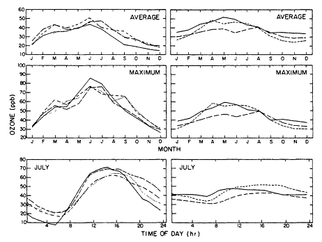
Figure 4-1
Seasonal and diurnal distributions of ozone at rural sites in the United States.
The upper panels show the seasonal distribution of daily average values; the
middle panels show monthly averages of the daily maximum values. The lower
panels show the diurnal behavior of ozone in July. The left panels show results
for four sites in the eastern United States from Aug. 1, 1977 to Dec. 31, 1979:
Montague, Massachusetts (solid); Scranton, Pennsylvania (dashed); Duncan
Falls, Ohio (dot dashed); and Rockport, Indiana (dot). The right panels show results
for three sites in the western United States from four years of measurements: Custer,
Montana (1979-1982, site at 1250 meters, short dashes); Ochoco, Oregon (1980-1983,
1350 meters, long dashes); and Apache, Arizona (1980-1983, 2500 meters, solid).
Source: Logan, 1988.
Page 102
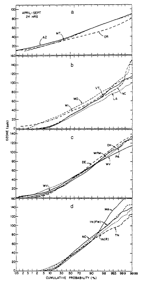
Figure 4-2
24-hour ozone cumulative probability distributions April 1-Sept. 30. (a) Western
NAPBN sites; (b) eastern NAPBN sites; (c) SURE sites; (d) Whiteface Mountain.
Sites are identified by state; results are plotted on probability paper; normally
distributed data define a straight line. Source: Logan, 1989.
Page 103
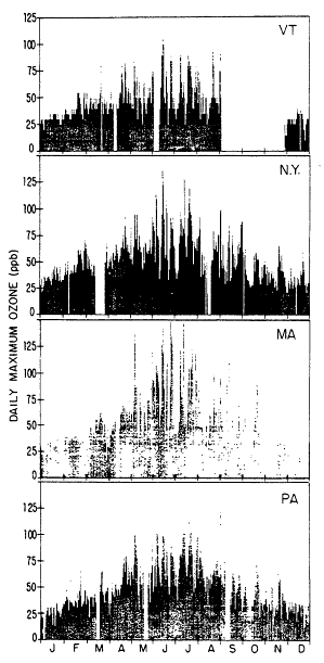
Figure 4-3
Time series of daily maximum ozone concentrations at rural sites
in the northeastern United States in 1979. Source: Logan, 1989.
Page 104
ber; they persisted for 3-4 days on average, with a range of 2-8 days, and were most common in June. Daily maximum ozone concentrations exceeded 90 ppb at more than half of the sites during these episodes and often were greater than 120 ppb at one or more sites. An analysis of the weather for each episode shows that high-ozone episodes were most likely in the presence of weak, slow-moving, persistent high-pressure systems as they migrated from west to east, or from northwest to southeast, across the eastern United States. Fast-moving and intense anticyclones (highs) were much less likely to promote the occurrence of ozone pollution episodes. The analysis of 2 complete years of data strengthens the conclusions of the case studies discussed earlier. There are no indications that either the weather or the ozone concentrations in 1978 and 1979 were particularly anomalous, although the concentrations could have been somewhat above average in 1978 (Logan, 1989).
The influence of the paths of anticyclones on the spatial pattern of ozone in the eastern two-thirds of the United States was examined by Vukovich and Fishman (1986). They showed maps of the mean diurnal maximum values of ozone for July and August of 1977-1981, using rural data where possible, and typical paths of anticyclones for each of these months. They concluded that if there is a persistent path for migratory high-pressure systems, the regions of high concentrations of ozone are associated with that pathway. An analysis of the climatology of anticyclones in July for 1950-1977 shows that the preferred track is across the northeast rather than across the southeast United States (Zishka and Smith, 1980). There was a downward trend in the number of anticyclones during this period.
The data discussed above show that there is a persistent blanket of high ozone in the eastern United States several times each summer, generally associated with stagnant high-pressure systems. Since rural ozone values commonly exceed 90 ppb on these occasions, an urban area need cause an ozone increment of only 30 ppb over the regional background to cause a violation of the NAAQS in a downwind area. Such increments have been demonstrated in the plume studies discussed earlier and in systematic studies of three urban areas (Kelly et al., 1986; Altshuller, 1988; Lindsay and Chameides, 1988).
Kelly et al. (1986) compared ozone concentration at a rural site outside Detroit with a site typically in the Detroit plume. For the upper quartile of ozone days in 1981, the ozone daily maximum was 104 ppb at the plume site, and the concentration at 1100 h was 47 ppb at the rural site. Kelly et al. argued that the plume generated 57 ppb ozone; the ozone maximum at the rural site was 73 ppb, 31 ppb below the plume's maximum value. On the day with the highest maximum ozone, 180 ppb, ozone concentrations were about 90 ppb at rural sites. Altshuller (1988) examined ozone formation in the St.
Page 105
Louis plume using 2 years of surface data from 12 sites. He compared the maximum ozone concentration at the station nearest the plume center and the average of the maximum ozone at upwind stations to obtain the change in ozone concentration (DO3). Monthly mean values of DO3 were 26-53 ppb, with an overall average of 45 ppb; high concentrations were most common in July and August, and the 90th-percentile value of DO3 was 80 ppb. In another study of the same data, Shreffler and Evans (1982) showed that upwind concentrations were 40-100 ppb and that DO3 appeared to be independent of the upwind concentrations. Finally, Lindsay and Chameides (1988) compared maximum ozone concentrations from stations upwind and downwind of Atlanta and at a rural site 125 km away. On days when urban ozone concentrations exceeded 100 ppb, the ozone concentration was 80-85 ppb at the upwind station and 110-125 ppb at the downwind station, suggesting that the city contributed 30-40 ppb above the immediate background. On these days, the ozone concentration at the rural site was 65 ppb, 20 ppb higher than average.
A study of the meteorological conditions associated with high-ozone days (above 80 ppb) in 17 cities demonstrated the regional nature of the problem, at least in the Northeast. Samson and Shi (1988) examined the wind flow for all days in 1983-85 when ozone exceeded 80 ppb in these cities, using trajectory calculations integrated backwards to the source region. They found that days with concentrations above 120 ppb were generally associated with low wind speeds, with the exception of Portland, Maine, where high-ozone days were moderately windy, presumably due to long-range transport of ozone from the south and west. The median distance the air had traveled in the previous 24 hours was about 500 km for the northeastern cities, suggesting long-range transport, but only 250 km for the southern cities. High-ozone days tended to occur over a longer season for the southern cities than for the northeastern cities (Figure 4-4).
Summary
Weather patterns play a major role in establishing conditions conducive to ozone formation and accumulation and in terminating episodes of high ozone concentrations. High ozone episodes are typically associated with weak, slow-moving high pressure systems traversing the central and eastern United States from west to east or from northwest to southeast. These episodes usually end with a frontal passage that brings cooler, cleaner air to the region. Clouds play an important role in the vertical redistribution of ozone and its precursors.
High ozone episodes last from 3-4 days on average, occur as many as 7-10
Page 106
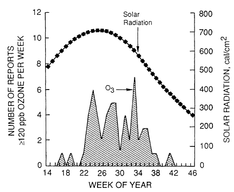
Figure 4-4a
The average number of reports of ozone concentrations ![]() ppb at
ppb at
the combined cities of New York and Boston from 1983 to 1985
(1April = week 14, 1 May = week 18, 1 June = week 22, 1 July = week 27,
1 August = week 31, 1 September = week 35, 1 October = week 40, 1
November = week 44). A representation of the annual variation in solar
radiation reaching the earth's surface at 40ºN latitude (units,
calories/cm2) is shown. Average over 1983-1985.
times a year, and are of large spatial scale: > 600,000 km2. Maximum values of non-urban ozone commonly exceed 90 ppb during these episodes, compared with average daily maximum values of 60 ppb in summer. An urban area need contribute an increment of only 30 ppb over the regional background during a high ozone episode to cause a violation of the National Ambient Air Quality Standard (NAAQS) in a downwind area. Such increments have been demonstrated in the studies described in this chapter. Given the regional nature of the ozone problem in the eastern United States, a regional model is needed to develop control strategies for individual urban areas. This
Page 107
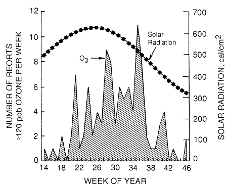
Figure 4-4b
The average number of reports of ozone concentrations ![]() ppb at
ppb at
the combined cities of Dallas and Houston, from 1983 to 1985.
(1 April = week 14, 1 May = week 18, 1 June = week 22, 1 July = week 27,
1 August = week 31, 1 September = week 35, 1 October = week 40, 1 November
= week 44). A representation of the annual variation in solar radiation reaching
the earth's surface at 30ºN latitude (units, calories/cm2) is shown.
Source: Samson and Shi, 1988.
need was recognized by EPA and led to the development of the Regional Oxidant Model, discussed in Chapters 10 and 11.
Regional models for ozone require a meteorological component that realistically describes the atmospheric wind field and its turbulence and mixing characteristics. Such a description is generally provided by prognostic meteorological models, as discussed in Chapter 10.


