Large-Scale Structures in Acoustics and Electromagnetics: Proceedings of a Symposium (1996)

Peter M. Pinsky

Stanford University

M. Malhotra

Stanford University

Lonny L. Thompson

Clemson University

In this paper the development of efficient computational methods for the exterior structural acoustics problem is considered from two standpoints. The first is a space-time finite element method for transient structural acoustics. The second is the development of efficient and robust iterative solution methods for large-scale problems in the frequency domain.

In the first part of this paper, a new space-time finite element approach for solving the coupled structural acoustics problem involving the interaction of vibrating structures submerged in an infinite acoustic fluid is described. The proposed method employs the simultaneous discretization of the spatial and temporal domains and is based on a new time-discontinuous variational formulation for the coupled fluid-structure system. In the proposed approach, the concept of space-time slabs is employed, which allows for discretizations that are discontinuous in time and offers greater discretization flexibility, e.g., through the use of space-time meshes oriented along space-time characteristics. In the space-time approach, increased algorithmic stability is obtained through the introduction of temporal jump operators, which give rise to a natural high-frequency dissipation required for the accurate resolution of sharp gradients in the physical solution. Additional stability is obtained by a least-squares modification. The order of accuracy of the solution depends directly on the order of the finite element spatial and temporal basis functions, which can be chosen to any accuracy for general unstructured discretizations in space and time. The resulting space-time approach, therefore, permits the development of a finite element method for transient structural acoustics with the desired combination of increased stability and high accuracy. Additionally, the proposed time-discontinuous Galerkin space-time method provides a natural variational setting for the incorporation of high-order accurate nonreflecting boundary conditions that are local in time. Since the temporal and spatial domains are treated in a consistent manner in the space-time variational equations, the method inherits a firm mathematical foundation from which rigorous a posteriori error estimates useful for reliable and efficient adaptive schemes may be established, (see, e.g., Johnson, 1990, 1993).

In the second part of this paper, we address issues relating to the efficient solution of large-scale matrix problems arising in steady state acoustics. Although considerable progress has been made in finite element methods for exterior problems in the frequency domain, efficient numerical algorithms for robust and accurate solution of large-scale acoustics problems still need to be developed. Although gradient-type iterative methods are an attractive alternative to direct methods for efficient solution of

large sparse matrix problems arising from finite element discretizations, the convergence of these methods deteriorates with increasing mesh density and increasing frequency of analysis. In such cases effective preconditioning becomes essential in order to accelerate iterative convergence. In the second part, we investigate a multilevel preconditioning approach that is based on the h-version of the hierarchical finite element method.

Consider the coupled system illustrated in Figure 9.1, consisting of the computational domain , composed of a fluid domain Ω_f, and structural domain Ω_s. The fluid boundary is divided into the fluid-structure interface boundary Г_i and the artificial boundary . The structural boundary is composed of the fluid-structure interface boundary Г_i and a traction boundary Gs. The infinite domain outside the artificial boundary is denoted by . The temporal interval of interest is and the number of spatial dimensions is d.

The structure is governed by the equations of elastodynamics, while the fluid equations are derived under the usual linear acoustic assumptions of an inviscid, compressible fluid with small disturbance. The strong form of the fluid-structure initial boundary-value problem is given by:

Find , and , such that

(9.1)

(9.2)

(9.3)

(9.4)

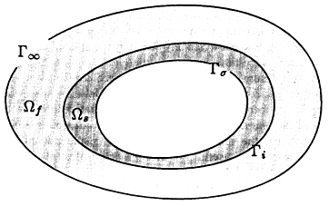
Figure 9.1 Coupled system for the exterior fluid-structure interaction problem, with artificial boundary enclosing the finite computational domain.

(9.5)

(9.6)

(9.7)

In the above, u(x, t) with is the structural displacement vector, σ is the symmetric Cauchy stress tensor, and (x,t) with is the scalar acoustic velocity potential. The phase velocity of acoustic wave propagation is denoted by c; ρ_s > 0 and ρ_f > 0 are the reference densities of the structure and fluid, respectively. A superposed dot indicates partial differentiation with respect to time t, and refers to the symmetric gradient. The acoustic pressure, p, and the acoustic velocity, ν, are related to the velocity potential by p = -ρ_f and . Equation (9.7) is the radiation boundary condition imposed on the artificial boundary , which approximates the asymptotic behavior of the solution at infinity, as described by the Sommerfeld radiation condition. Also, appropriate initial conditions are assumed corresponding to the above coupled second-order system of hyperbolic equations.

The development of the space-time method proceeds by considering a partition of the time interval, , of the form 0 = t₀ < t₁ <...< t_N = T, with . Using this notation, and are the nth space-time slabs for the structure and fluid respectively. For the nth space-time slab, the spatial domain is subdivided into (n_el)_n elements, and the interior of the e^th element is defined as . Figure 9.2 shows an illustration of two consecutive space-time slabs Q_n-1 and Q_n for the fluid where the superscript is omitted for clarity.

Within each space-time element, the trial solution and weighting function are approximated by pth-order polynomials in x and t. These functions are assumed C⁰(Q_n) continuous throughout each space-time slab, but are allowed to be discontinuous across the interfaces of the slabs. This feature of the time-discontinuous method allows for the general use of high-order elements and spectral-type interpolations in both space and time. The collections of finite element interpolation functions are given by the spaces as follows:

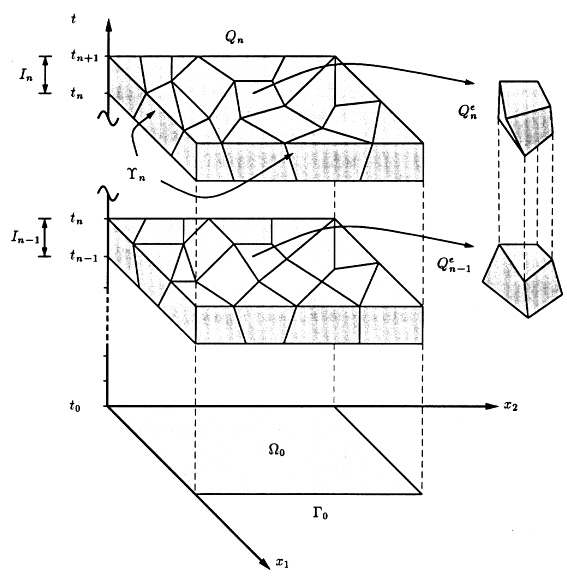
Figure 9.2 Illustration of two consecutive space-time slabs with unstructured finite element meshes in space-time.

where denotes the space of pth-order polynomials and C⁰ denotes the space of continuous functions. For clarity, only natural boundary conditions are employed. As a result the trial function spaces and weighting spaces are identical, i.e., and . Before stating the space-time variational equations, it is useful to introduce the following notation:

The interpretation of other similar terms may be inferred from these. The L₂ norm is denoted by . A natural measure of stability for the coupled structural acoustics problem is the total energy for the system:

where and denote energy of the elastic structure and of the acoustic fluid, respectively.

The space-time variational formulation is obtained from a weighted residual of the governing equations and incorporates time-discontinuous jump terms. The specific form of this new formulation is designed such that unconditional stability for arbitrary space-time finite element discretizations can be proved through a functional analysis of the method. The time-discontinuous Galerkin formulation can be stated formally:

Within each space-time slab, n = 0,1, . . . , N - 1, find , such that when , the following coupled variational equations are satisfied:

where

In the operator G_s, the terms evaluated over Ω_s × I_n weakly enforce the momentum balance in the structure while in G_f, the terms evaluated over Ω_f × I_n weakly enforce the scalar wave equation over the interior domain of the space-time slab. Fluid-structure interaction is accomplished through the

coupling operators defined on the fluid-structure interface Г_i × I_n. The operator incorporates the time-dependent radiation boundary conditions on the boundary , and will be described later in the next section (on Exact Nonreflecting Boundary Conditions).

An important component in the success of the space-time method is the incorporation of discontinuous temporal jump terms, , at each space-time slab interface. These jump operators weakly enforce initial conditions across time slabs and are crucial for obtaining an unconditionally stable algorithm for unstructured space-time finite element discretizations with high-order interpolations. The specific form of these jump operators is designed such that a natural norm emanates from the variational equation and satisfies a strong coercivity condition. From a Fourier analysis, it can be shown that the jump operators introduce beneficial numerical dissipation for frequencies above the spatial resolution limit.

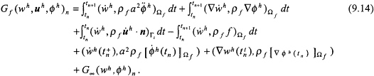
The method is applied in one space-time slab at a time; data from the end of the previous slab are employed as initial conditions for the current slab. Matrix equations are obtained by introducing space-time finite element approximations for u^h(x,t) = N_s(x,t)d and ^h(x,t) = N_f(x,t). In these expressions and are basis functions defined over a space-time slab, and d and are global solution vectors. Inserting into the variational (9.13) and (9.14) leads to the coupled system of algebraic equations to be solved in sequence for each time interval :

where K_s is the matrix emanating from the structural operator G_s, K_f is the matrix emanating from the fluid operator G_f, and A is the fluid-structure coupling matrix:

where and shape functions for the structure and fluid respectively.

New time-dependent nonreflecting boundary conditions, which are exact for the first N spherical wave harmonics on , have been derived recently (Thompson and Pinsky, 1994, 1995a; Thompson, 1994). Two alternative sequences of time-dependent nonreflecting boundary conditions have been obtained; the first involves both time and spatial derivatives (local in time and local in space version), and the second involves time derivatives while retaining a spatial integral (local in time and nonlocal in space version).

In the first version, a local in time counterpart to the spatially nonlocal DtN map is derived in Thompson (1994) and Thompson and Pinsky (1995a), which exactly represents the first N spherical wave harmonics. This new sequence of boundary conditions retains the nonlocal spatial integral, yet replaces the time-convoluted DtN map with higher-order local time derivatives. This form of time-dependent boundary conditions has the advantage that, when implemented in the time-discontinuous

finite element formulation, standard interpolation functions may be used for both the space and time variables.

The second version starts from the localization of the acoustic impedance relation, the Dirichlet-to-Neumann (DtN) map in the frequency domain. In Thompson (1994) and Thompson and Pinsky (1995b), it is shown that when the solution on the boundary contains only a finite number of spherical harmonics, then such a transformation gives an exact condition that is local in both x and t. The sequence of local boundary conditions is obtained by truncating the DtN map. Time-dependent boundary conditions are then obtained through the application of an inverse Fourier transform. This new sequence of local time-dependent boundary conditions provides increasing accuracy with order N, which, however, is also a measure of the difficulty of implementation. In general, the Nth-order condition contains all the even tangential and temporal derivatives up to order 2(N-1). Because the time-discontinuous formulation allows for the use of C⁰ interpolations to represent the high-order time derivatives, it is possible to implement this sequence of time-dependent absorbing boundary conditions up to any order desired. However, for high-order operators in the sequence extending beyond , the lowest possible order of spatial continuity on the artificial boundary that can be achieved after integration by parts is C^N-2. For these high-order operators, a layer of boundary elements adjacent to possessing high-order tangential continuity on is needed. Further details on the finite element implementation of these boundary conditions using the space-time formulation are described in Thompson (1994).

In this section, results are summarized from a stability analysis of the space-time finite element formulation for the exterior structural acoustics problem. In the absence of forcing terms, i.e., and f = 0 and for , it has been proved in Thompson (1994) and Thompson and Pinsky (1995b) that the following energy decay inequality holds for the coupled space-time formulation:

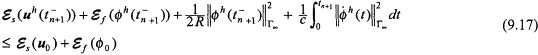
for n = 0,1,2,..., N - 1. In the above inequality, and were defined earlier in Yserentant (1986) and Zienkiewicz et al. (1981) and denote the energy for the elastic structure and acoustic fluid respectively. Equation (9.17) states that the total energy in the fluid-structure system, plus the energy absorbed through the radiation boundary, is always less than or equal to the initial energy in the system. A corollary to this estimate is that the computed total energy for the system plus the radiation energy absorbed through the artificial boundary at the end of a time step is always less than or equal to the total energy at the previous time step for arbitrary step sizes, i.e.,

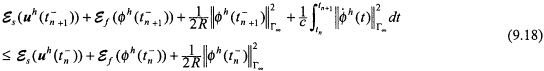
for n = 0,1,2,..., N - 1. Results (9.17) and (9.18) both imply that the space-time formulation presented is unconditionally stable. See Thompson (1994) for an analogous result for the interior problem where no radiation boundary conditions are present.

For additional stability, local residuals of the governing differential equations in the form of least-squares may be added to the Galerkin variational equations. The Galerkin/Least-Squares addition to the variational equation for the fluid (9.14) is

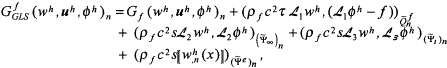
where () is the residual for the wave equation, () is the radiation boundary residual, and () is the interface boundary residual. In the above expressions, a tilde refers to integration over element interiors and τ and s are local mesh parameters designed to improve desirable high-frequency numerical dissipation without degrading the accuracy of the underlying time-discontinuous Galerkin method. For the structural equation (9.13), similar least-squares terms are added (see Thompson, 1994). Consistency of both the underlying method and the least-squares addition is clear from the fact that a sufficiently smooth exact solution of the coupled initial/boundary-value problem as stated in (9.1)-(9.7), satisfies the variational equations (9.13), (9.14), and (9.19) identically.

To study the convergence rates of the space-time finite element formulation for the exterior structural acoustics problem the following space-time mesh size parameters are introduced. For the structural domain Ω_s ,h_s = max{c_LΔt,Δx} where c_L is the dilatational wave speed and Δx and Δt are maximum element diameters in space and time, respectively. For the fluid domain Ω_f, h_f = max{cΔt,Δx} where c is the acoustic wave speed. Assuming that the exact solution to the strong form of the initial boundary value problem with is sufficiently smooth in the sense that

and assuming standard finite element interpolation estimates hold, then it has been proved in Thompson (1994) and Thompson and Pinsky (1995b) that the following error estimate holds for the time-discontinuous Galerkin Least-Squares formulation,

where k and p are the finite element interpolation orders for the structure and fluid respectively. In the above, the error is defined as

and c(u) and c() are values that are independent of the mesh size parameters h_s and h_f. The norm in which convergence is measured is given by

In the above expression is the residual for the structure. This norm emanates naturally from the coupled fluid-structure variational equations (9.13) and (9.14) together with the least-squares operators discussed above. The error estimate is optimal in the sense that the finite element error converges at the same rate as the interpolate. This result indicates that the error for the coupled system is controlled by the convergence rates in both the structure and the fluid. In other words, for an accurate solution to the coupled fluid-structure problem, discretizations for both the structural domain and the fluid domain must be adequately resolved.

Convergence rates are verified numerically by calculating the response of the one-dimensional wave equation in the interval . On the boundary L = 4, the exact nonreflecting boundary condition

is imposed. The left end (x = 0) is fixed. A transient pulse of the form

is initiated at x₀ = 2.4 with wavelength λ = 0.8. The response was calculated for the time interval . Each space-time slab was discretized with a uniform mesh of 160 biquadratic elements. Figure 9.3 shows the error computed using the Galerkin Least-Squares formulation at time T = 1.8. This result confirms that a cubic rate of convergence is obtained as predicted by (9.20).

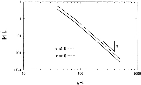
Figure 9.3 Convergence of the numerical error employing the Q2 element; h = h _f is the element mesh size parameter. Results confirm the high-order convergence rate (2p - 1) = 3 for p = 2.

A numerical example is presented to demonstrate the effectiveness of the time-discontinuous space-time finite element method to accurately model transient scattering from geometrically complex structures. The problem investigated also assesses the performance of the local nonreflecting boundary conditions. For all the numerical results presented, the GLS mesh parameters are set to zero and standard quadratic finite element shape functions are used in both the time and space dimensions.

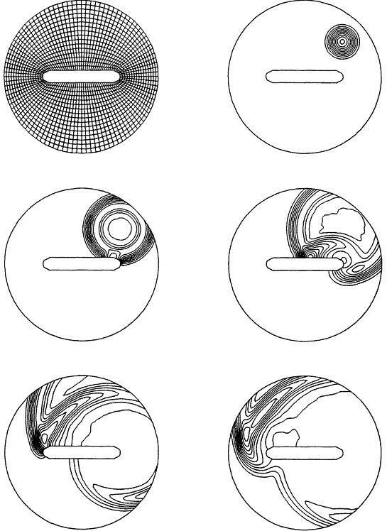
Consider the time-dependent scattering from a rigid cylinder with conical-to-spherical end caps and a large length to diameter ratio. Figure 9.4 illustrates the finite element spatial discretization of the computational domain bounded internally by the lateral projection of the benchmark cylinder and externally by a circular artificial boundary. A total of 1,600 space-time elements are used for this example. For this two-dimensional problem, we consider the the following second-order local time-dependent boundary operator (Pinsky et al, 1992):

The pulse f = δ(x₀,y₀) sin ωt and is positioned inside the computational domain, simulating an oblique incident wave during a short time period. The numerical simulation is continued until just prior to reaching the practical disappearance of the signal from the domain. This example represents a challenging problem where the multiple-scales involving the ratio of the wavelength to cylinder diameter and cylinder length dimension play a critical role in the complexity of the resulting scattered wave field.

The numerical simulation starts with the initial pulse shown in Figure 9.4 at t = 3. The accompanying figures show the contours of the scattering phenomena from the cylinder with homogeneous Neumann boundary conditions on the wet surface, i.e., ''rigid'' boundary conditions. At t = 6 the incident pulse has expanded in a cylindrical wave and has just reached the boundaries of the rigid cylinder. At the artificial boundary, the wave front is allowed to pass through the boundary with no reflection. At t = 9, the wave has begun to reflect off the rigid boundary, creating a complicated backscattered wave. As time passes, the originally cylindrical incident wave has been scattered into a part that travels along the upper part of the cylinder, and a part that diffracts around the backside.

In the second part of this paper, we consider efficient methods for the solution of large-scale matrix problems that arise from finite element methods for structural acoustics. Direct solution techniques become expensive for solving large systems of linear equations due to excessive growth in computational and storage requirements. Iterative solution strategies are an attractive alternative in these situations. Also, unlike direct methods, characteristic computational kernels associated with iterative solution methods parallelize very efficiently, making them even more attractive for use on modern vector and parallel computers. However, for matrix problems arising from finite element discretizations in acoustics, the convergence of gradient-type iterative methods deteriorates under increasing mesh density and increasing frequency. Under these circumstances, effective preconditioning becomes essential. For

effective preconditioning of the Helmholtz operator we examine a novel approach that is based on an understanding of the properties of finite element discretization of a second-order elliptic differential operator.

As a model problem we consider a linear, second-order, elliptic partial differential equation along with specified boundary conditions,

with the boundary of the domain . The variational form of the problem is expressed as follows: Find satisfying u = g on Г_g such that a( u,v) =f(v) holds satisfying v = 0 on Г_g. The bilinear functional a(.,.) is defined on the Sobolev space H and corresponds to the differential operator ; f(.) is a linear functional corresponding to the forcing function and specified flux boundary conditions. Introducing a finite element discretization of the domain and choosing a basis on this discretization, the approximate statement of the variational problem becomes: Find satisfying u^h = g on such that

holds satisfying v^h = 0 on . By employing the Galerkin approach, the discrete system of equations to be solved is Kd = f, where K_ij = a(_i,_j) and f_j = f(_j). If a(.,.) is evaluated using the usual nodal basis consisting of Lagrange polynomials, shown in Figure 9.5b, then the spectral condition number of K grows as O(h^-2), where h is the characteristic mesh size (see, e.g., Axelsson and Barker, 1984). However, for an appropriate set of h-hierarchical basis functions the condition number grows as O(logh^-1)² (Yserentant, 1986). In the h-hierarchical approach, basis functions of the same polynomial order are introduced in a hierarchic fashion corresponding to nodes in the interior of an element (see Figure 9.5a). Although not necessary, it may be useful to consider such interior nodes as those arising from refinement of an initial coarse mesh. Alternatively, it is useful to think of these nodes as being associated with a "multilevel splitting" of a given mesh (Yserentant, 1986).

Using these multiple levels, the hierarchical basis can be defined as follows: (1) basis functions at the coarsest level, level 1, consist of the nodal basis functions, and (2) the hierarchical basis at any level j > 1 consists of nodal basis functions corresponding to nodes in that level which are not present in any of the coarser levels, together with the hierarchical basis for level j - 1. This recursive definition leads to a set of basis functions that is complete and unique. We now describe transformation matrices that relate the nodal basis with an equivalent set of h-hierarchical basis functions.

Figure 9.5 (a) h-Hierarchical linear shape functions introduced with two refinement levels.

(b) An equivalent nodal basis for the final mesh with linear Lagrange polynomials.

Consider a function approximated on a given finite element mesh with n unknowns (or degrees of freedom) using nodal and hierarchical basis functions as

respectively. Let = { ₁(x), ₂(x),..., _n(x)}^T and Ψ = {Ψ₁(x),Ψ₂ (x),..., Ψ_n(x)}^T denote column vectors comprising nodal and hierarchical basis functions respectively. We are interested in the linear transformation matrix P such that Ψ = P. For the case of two levels, it is easy to show that the nodal and hierarchical basis functions are related as

where n₁ is the number of nodes in Level 1, and nodes in Level 1 are assumed to be numbered before those in Level 2; and are square identity matrices of size n₁ and n - n₁; and F is a sparse matrix containing the interaction of hierarchical shape functions between the two levels. To generalize (9.32) for the case of multiple levels, recall the definition of the hierarchical basis functions. Due to the

recursive construction of the hierarchical basis, the transformation matrix in the case of j > 2 levels can be stated as

where P_k is the transformation between the nodal basis on Level k+1, the hierarchical basis on nodes in Level k and Level k+1. Each P_k essentially has the same structure as P₁ (shown in (9.32)).

Now consider the solution of our nodal basis finite element equations Kd = f. In order to achieve improved conditioning of the matrix equations, we start by employing hierarchical basis functions in the bilinear form a(.,.) of (9.28). Now, using (9.33), introduce nodal basis functions Φ in place of to get a relation between K and its equivalent representation in the hierarchical basis ,

If we choose P^-1 and P^-T as left and right preconditioners, the hierarchical basis preconditioner can be stated as M_HB = (P^TP)^-1. Such a construction of the hierarchical basis preconditioner from transformation matrices was obtained by Yserentant (1986). It is interesting to note that the matrix entries in M_HB are independent of the coefficients that appear in the differential operator . In order improve this situation, we combine diagonal scaling with the preconditioner M_HB. Although diag () is not easily available, it is frequently useful (Greenbaum et al., 1989) to employ instead diag (K) in the following way:

Another approach in enhancing M_HB becomes evident if we consider the block form of . Ordering all nodes in coarsest level first, we form the preconditioner

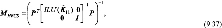
where the operator represents an approximate solution of unknowns associated with nodes in the coarsest level, and the block matrix , with _i and _i being the basis functions corresponding to nodes in Level 1. We compare the performance of preconditioners (9.36) and (9.37) in our numerical examples.

The use of a preconditioner in conjunction with a gradient-type iterative method requires solving a system of equations, of the form Mz = r, at each step of the iteration. An attractive feature of the preconditioners M_HB or M_HBDS is that solving for z doesn't require a matrix inversion, and only matrix-vector products of the form

need to be evaluated. Since the preconditioner appears in the above operations only, significant reductions in storage and computational costs can be realized if these matrix-vector products are computed directly and the explicit calculation of P and P^T is avoided. This is a key algorithmic feature that was also exploited in Yserentant (1986). On unstructured grids, the preconditioning steps in equation (9.38) can be performed using nearest-neighbor type connectivity data between successive hierarchical levels. Such a procedure entails only a limited amount of additional storage of O(n_np) words, and a computational complexity of O(n_np) flops. Here n_np denotes total number of mesh points. See Malhotra and Pinsky (1995) for a description of data-structures and algorithms for efficient implementations on serial and distributed memory computers.

An important ingredient in the construction of hierarchical basis preconditioners is the choice of a multilevel splitting associated with the finite element mesh on which the problem needs to be solved. Multiple grid levels inherent in such a splitting arise quite naturally in h-adaptive finite element computations if nested mesh refinement is employed. However, in applying the preconditioning approach to indefinite problems, a more careful selection of grid levels is required. Results, based on both a priori convergence analyses (Schatz, 1974) as well as dispersion analyses (Thompson, 1994) of finite element discretizations, indicate that for indefinite problems it is essential that the mesh size be sufficiently small in order to maintain accuracy of finite element approximations. For the Helmholtz equation, results of one-dimensional dispersion analysis indicate a limit of resolution given by where k is the wavenumber for linear basis functions. In our numerical tests on two-dimensional scattering problems using multilevel hierarchical grids, the coarse grid was chosen to satisfy this limit of resolution.

It is noteworthy that the preconditioning approach described here is not directly based on a "splitting" or "factorization" of the large sparse coefficient matrix K. The hierarchical basis preconditioners, therefore, can also be employed in conjunction with highly storage-efficient matrix-free implementations of a gradient-type iterative algorithm. Matrix-free iterative approaches involve calculating characteristic computational kernels required in the iterative method without the explicit assembly of any global matrix, which enables substantial storage reductions. This is particularly useful in

the context of acoustics, where a matrix-free representation of the non-local DtN contribution allows the use of this highly accurate boundary condition without any storage penalties associated with its nonlocal nature (Malhotra and Pinsky, 1995).

A canonical problem in structural acoustics is the scattering of plane waves from a rigid body submerged in a fluid of infinite extent. Here we consider two-dimensional plane-wave scattering from a rigid cylinder with conical-to-spherical end caps and a large length to diameter ratio as shown in Figure 9.6. The governing equations are:

(9.39)

(9.40)

(9.41)

In the above equations, p is the unknown acoustic pressure in the fluid domain , k is the wavenumber, and n denotes unit outward normals from respective boundaries. Equation (9.41) represents the impedance of the infinite acoustic medium, exterior to , through the boundary operator . We employ an exact representation of the radiation impedance by choosing to be the Dirichlet-to-Neumann (DtN) map (Keller and Givoli, 1989); for details on finite element modeling of (9.39)-(9.14), see Harari (1991). We consider plane waves incident along the length of the cylinder such that p_inc = e^ikx, where and x is the coordinate along the length of the cylinder. As our basic iterative method, we employ the complex-symmetric preconditioned quasi-minimal residual (QMR) iterative method (Freund and Nachtigal, 1991; Freund, 1992). Iterations are stopped when the true residual at iteration k satisfies .

The effect of mesh refinement is examined first by fixing the frequency of analysis at k = π / 6 and solving the problem on three successively refined meshes. In order to construct M_HBDS, an initial coarse

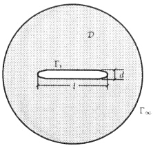
Figure 9.6 Two-dimensional trace of a rigid cylinder with end caps, l / d = 8.

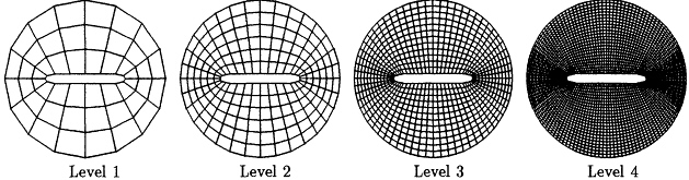
Figure 9.7 Multiple grid levels for the scattering example: solution on mesh with 3,200 unknowns, kd = π / 6.

mesh of 3 × 16 elements (radial × circumferential elements) was used and intermediate mesh levels were obtained by successive uniform refinement (Figure 9.7). We denote by "HB Levels" the total number of hierarchical levels used to construct the transformations from the nodal to the hierarchical basis.

Table 9.1 summarizes the number of iterations required for convergence using various preconditioners. Observe that the unpreconditioned algorithm, denoted by M_I, suffers substantial deterioration in iteration count as the mesh size decreases. Diagonal preconditioning, M_D, offers little improvement. The performance of M_HBDS appears to be almost mesh-independent. Similar behavior is observed for analysis at kd= π / 2 and kd = π illustrated in Figure 9.8.

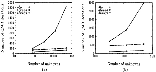
Figure 9.8 Convergence with mesh refinement for (a) kd = π / 2, (b) kd = π.

Next, we examine the effect of increasing frequency on the performance of various preconditioners. Figure 9.9 shows the number of iterations needed for convergence as the wavenumber is increased to kd = π / 2 + and then kd = π. Although M_HBDS performs better than diagonal scaling, the iteration counts for M_HBDS do not remain as favorable when the wavenumber increases to kd = π. However, the preconditioner M_HBDS accounts for the deterioration in convergence with frequency increase and leads to a rate of convergence that is almost both mesh- and frequency-independent.

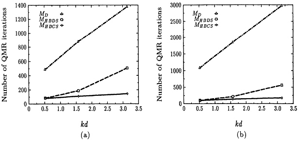
Figure 9.9 Convergence with frequency increase for meshes with unknowns (a) n = 12544, (b) n = 49664.

In this paper, a new space-time finite element method for solution of the transient structural acoustics problem in exterior domains has been presented. The formulation is based on a new time-discontinuous Galerkin Least-Squares variational equation for both the structure and the acoustic fluid together with their interaction. The resulting space-time algorithm gives for the first time a general solution to the fundamental problem of constructing a finite element method for transient structural acoustics with unstructured meshes in space-time and the desired combination of increased numerical stability and high accuracy.

Desirable attributes of the new computational method for transient structural acoustics include a natural framework for the design of rigorous a posteriori error estimates for self-adaptive solution strategies for unstructured space-time discretizations, and the implementation of high-order accurate time-dependent nonreflecting boundary conditions. Furthermore, through the use of acoustic velocity potential and structural displacement as the solution variables, the space-time method is unconditionally stable and converges at an optimal rate in a norm that is stronger than the total energy norm. High-order accuracy is obtained simply by raising the order of the space-time polynomial basis functions; both standard nodal interpolation and hierarchical shape functions are accommodated.

In the second part of this paper, a preconditioning approach based on exploiting the properties of h-hierarchical basis functions associated with a multilevel splitting of a given finite element mesh was considered. Numerical tests were performed for the solution of two-dimensional scattering problems in acoustics in order to examine iterative convergence rates obtained with various preconditioners. These tests indicate that convergence rates predicted by theoretical asymptotic bounds, which motivate the formation of h-hierarchical basis preconditioners, are actually realized on practical discretizations for problems in acoustics. Moreover, by combining hierarchical basis transformations with the solution of a coarse problem, we achieve iterative convergence rates for the Helmholtz equation that are almost frequency- and discretization-independent. The basis transformations inherent in these preconditioners can also be applied efficiently in conjunction with matrix-free gradient-type iterative algorithms. We have found such an approach to be very efficient and quite promising for solving very large-scale problems in exterior structural acoustics on distributed-memory parallel computers.

Axelsson, O., and V.A. Barker, 1984, Finite Element Solution ofBoundary Value Problems: Theory and Computation, Orlando, Fla.: Academic Press.

Freund, R.W., 1992, "Conjugate gradient-type methods for linear systems with complex symmetric coefficient matrices,"SIAM J. Sci. Statist.Comput.13, 425-448.

Freund, R.W., and N.M. Nachtigal, 1991, "QMR: A quasi-minimal residual method for non-Hermitian linear systems,"Numer. Math.60, 315-339.

Greenbaum, A., C. Li, and H.Z. Chao, 1989, "Parallelizing preconditioned conjugate gradient algorithms,"Comput. Phys. Commun.53, 295-309.

Harari, I., 1991, Computational Methods for Problems of Acousticswith Particular Reference to Exterior Domains, PhD Thesis, Stanford University.

Johnson, C., 1990, "Adaptive finite element methods for diffusion and convection problems,"Comput. Methods Appl. Mech. Eng.82, 301-322.

Johnson, C., 1993, "Discontinuous Galerkin finite element methods for second order hyperbolic problems,"Comput. Methods Appl. Mech.Eng.107, 117-129.

Keller, J.B., and D. Givoli, 1989, "Exact non-reflecting boundary conditions,"J. Comput. Phys.82(1), 172-192.

Malhotra, M., and P.M. Pinsky, 1995, ''Parallel preconditioning based on h-hierarchic finite elements with application to acoustics,'' in preparation.

Pinsky, P.M., L.L. Thompson, and N.N. Abboud, 1992, "Local high order radiation boundary conditions for the two-dimensional time-dependent structural acoustics problem,"J. Acoust. Soc. Am.91(3), 1320-1335.

Schatz, A.H., 1974, "An observation concerning Ritz-Galerkin methods with indefinite bilinear forms,"Math. Comput.28, 959-962.

Thompson, L.L., 1994, Design and Analysis of Space-Time and GalerkinLeast-Squares Finite Element Methods for Fluid-Structure Interactionin Exterior Domains, PhD Thesis, Stanford University.

Thompson, L.L., and P.M. Pinsky, 1994, "New space-time finite element methods for fluid-structure interaction in exterior domains,"ComputationalMethods for Fluid/Structure Interaction178, 101-120.

Thompson, L.L., and P.M. Pinsky, 1995a, "A space-time finite element method for structural acoustics in infinite domains, part i: Formulation, stability, and convergence,"Comput. Methods Appl. Mech. Eng., submitted.

Thompson, L.L., and P.M. Pinsky, 1995b, "A space-time finite element method for structural acoustics in infinite domains, part ii: Exact time-dependent non-reflecting boundary conditions,"Comput. MethodsAppl. Mech. Eng., submitted.

Yserentant, Harry, 1986, "On the multi-level splitting of finite element spaces,"Numer. Math.49, 379-412.

Zienkiewicz, O.C., D.W. Kelly, J. Gago, and I. Babuška, 1982, "Hierarchical finite element approaches, error estimation and adaptive refinement." In: The Mathematics of Finite Elements and Applications IV, J.R. Whiteman (ed.), pp. 314-346, New York: Academic Press.