
Failures, Fantasies, and Feats in the Theoretical/Numerical Prediction of Ship Performance
L.Larsson,1,2 B.Regnström,2 L.Broberg,2 D.-Q.Li,1,3 C.-E.Janson2
(1Chalmers University of Technology, 2FLOWTECH International AB, 3SSPA Maritime Consulting AB, Sweden)
Abstract
The status of CFD in hydrodynamics is reviewed. After a brief historical survey a theoretical introduction is given to potential flow panel methods and methods based on the Reynolds-Averaged Navier-Stokes equations. Present capabilities are then discussed, and the attainable accuracy in the prediction of waves, wave resistance, local flow, viscous resistance and propeller effects is assessed. Prospects for improvements, based on present research in grid generation, free surface flows, turbulence modelling, propeller flows and full scale predictions are outlined. Finally, the exciting long term possibilities are presented and a number of conclusions drawn.
1. Background
The modern research in computational hydrodynamics is intimately linked to the development of the computer, and methods based on massive “number crunching” have replaced the more elegant, but less general, analytical methods developed during the first half of this century. One of the first representatives of the new approach is the Hess and Smith method (1), presented in 1962. For the first time it became possible to compute the 3-D potential flow around arbitrarily shaped bodies with an exact boundary condition applied on the hull surface. The method was later generalized to include lift, certainly important for aerodynamic flows, but of more hydrodynamic interest was the introduction of the free surface by Dawson in 1977 (2). Dawson’s method, although based on a linearization of the free surface boundary conditions, soon became an important tool in ship design, and it was the starting point for research at many organizations.
One of the main objectives of the research was to remove the free surface linearization and to introduce exact boundary conditions satisfied at the exact location of the wavy free surface. In a series of PhD projects at Chalmers University of Technology this route was followed, and in 1989 a paper was presented (Larsson, et al (3)), where the major results of the first three projects were presented. Recently, the fourth project was finished by Janson (4) and a robust non-linear method based on this research is now available in the commercial CFD package SHIPFLOW (5). A parallel development was carried out at MARIN, Holland, and in 1996 Raven (6) presented a non-linear method of a similar kind. In the opinion of the authors this development is now close to its limits. Raven’s and Janson’s theses work, based on all previous efforts in the same area, have led to methods which cannot be much improved under the potential flow approximation. To proceed further, viscosity has to be taken into account.
In the sixties the viscous flow research was directed towards 2-D boundary layer theory and by the end of the decade several methods for arbitrary pressure gradients were available. This research continued for 3-D methods during the seventies and an evaluation was made at a workshop organized by one of the authors in Gothenburg in 1980, see Larsson (7). Like in a previous workshop on wave resistance held in the Washington DC in 1979 a number of methods were applied to some well specified test cases and the differences were analysed in view of the differences in the
underlying theory. It turned out that most methods produced acceptable results for the major part of the boundary layer along the hull, while all failed completely near the stern. This prompted several groups to start research on less approximate methods based on the Reynolds-Averaged Navier-Stokes (RANS) equations. By the end of the eighties a number of RANS methods for ship flows had been developed and in a new Gothenburg workshop (Larsson et al (8)), a considerable improvement was noted in the capability to predict the stern flow. This improvement was verified at a new workshop organized by Kodama et al (9) in Tokyo in 1994, where, however, the most important breakthrough was the introduction of the free surface in the RANS methods. No less than 10 methods now featured this capability; a result of the research in several groups since the mid-eighties, as will be further discussed below.
There is no doubt that the most important developments to be expected in the future will be in the viscous flow area. With the increasing power of computers more advanced methods will become available, based either on the Large Eddy Simulation (LES) technique, where the large turbulent eddies are computed and only the smaller ones modelled, or on the DNS technique, where all eddies and scales are computed.
In the following, we will first give a brief theoretical introduction to potential flow panel methods and methods of the RANS type. This will be in Section 2. Thereafter, in Section 3 an assessment will be made of current CFD capabilities. Ongoing research and short term prospects for improvements will be addressed in Section 4, and in Section 5 a forecast will be made of the exciting long term possibilities. Finally, a number of conclusions will be drawn. The emphasis will be on resistance and powering, but some reference will be made to research in other areas of ship hydrodynamics as well.
2. Theory
In this Section a short theoretical introduction will be given, covering potential flow panel methods and Reynolds-Averaged Navier-Stokes methods. For obvious reasons the description has to be brief. This holds particularly for the RANS part, which will be further discussed in later Sections.
2.1 Potential Flow Panel Methods
The flow is assumed steady, irrotational and incompressible. A Cartesian coordinate system is employed, where the origin is at the bow and at the undisturbed free surface level, x downstream, y to starboard and z upwards. U and q represent the undisturbed and disturbed velocities, respectively. Defining a velocity potential ![]() by
by
(1)
this potential will satisfy the Laplace equation
(2)
On the hull boundary the normal velocity is zero
(3)
and on the free surface boundary a similar relation holds. This kinematic condition may be written as
(4)
where h=h(x,y) is the equation for the wavy surface.
A dynamic free surface condition may be obtained from the continuity of stresses across the interface. In a potential flow, this condition degenerates to the simple statement that the pressure must be atmospheric at the surface, and without loss of generality this pressure may be set to zero. Neglecting surface tension and applying the Bernoulli equation the dynamic free surface boundary condition may be written
(5)
At infinity the velocity is undisturbed
(6)
g is the acceleration of gravity and R is the distance from the origin.
Finally, the radiation condition states that no below, this condition is enforced numerically. waves may be transmitted upstream. As explained
The free surface boundary conditions are nonlinear and they have to be applied at an initially unknown surface. This may be accomplished as follows. Assume that an approximate solution ![]() is known. Introduce small disturbances
is known. Introduce small disturbances ![]() and δh and expand equations (4) and (5) in these quantities around the known solution. Delete terms of higher order. This yields, (see Janson (4))
and δh and expand equations (4) and (5) in these quantities around the known solution. Delete terms of higher order. This yields, (see Janson (4))
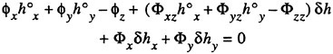
(7)
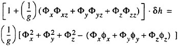
(8)
where ![]() has been replaced by
has been replaced by ![]() . In thin ship theory the known solution is taken as Φ=Ux, ho=0, i.e. the undisturbed flow and a flat free surface. Dawson used Φ=ΦDΜ, ho=0, where ΦDM stands for the double model solution. In SHIPFLOW (3), (4), (5),
. In thin ship theory the known solution is taken as Φ=Ux, ho=0, i.e. the undisturbed flow and a flat free surface. Dawson used Φ=ΦDΜ, ho=0, where ΦDM stands for the double model solution. In SHIPFLOW (3), (4), (5), ![]() and ho,n+1=hn, where n is the iteration number in an iterative sequence, which starts with the double model solution, as in Dawson’s method. When the process converges the neglected quantities in equations (7) and (8) go to zero and the position where the free surface boundary conditions are applied approaches the correct one. In the limit, the exact solution is thus obtained. Note that very non-linear effects, like spray and wave breaking cannot be predicted.
and ho,n+1=hn, where n is the iteration number in an iterative sequence, which starts with the double model solution, as in Dawson’s method. When the process converges the neglected quantities in equations (7) and (8) go to zero and the position where the free surface boundary conditions are applied approaches the correct one. In the limit, the exact solution is thus obtained. Note that very non-linear effects, like spray and wave breaking cannot be predicted.
The problem posed by the field equation (2) and the boundary conditions (3), (6), (7) and (8) is solved by a boundary integral technique where sources are distributed on the hull and part of the free surface. Optionally, the free surface sources may be raised a certain distance above the surface (desingularisation, (4) (6)). The ![]() potential at any point due to the distribution of sources is
potential at any point due to the distribution of sources is
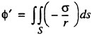
(9)
where σ is the source density, r is the distance from a point on the surface to the field point and S is the hull and free surface (covered part). Note that the sources satisfy both the field equation (2) and the infinity condition (6) for all σ. The solution thus has to be found from the three remaining boundary conditions (3), (7) and (8).
The problem is discretized by representing the hull and the (possibly raised) free surface by quadrilateral panels, each of which having an individual distribution of sources. In the SHIPFLOW code (3), (4), (5) two options exist: either the panels are assumed flat and the source strength constant on each panel (first order method), or the panels are parabolic with a linear variation in the source strength (second order method). In both cases the number of unknowns is equal to the number of panels. Since the boundary condition is applied at one point (the collocation point) on each panel the problem is closed.
A final free surface boundary condition is obtained by solving (8) for δh, differentiating this relation with respect to x and y and introducing all three quantities in (7). Second derivatives of the unknown potential ![]() will then appear and these may be handled in two principally different ways. Either (9) may be differentiated twice to give analytical expressions for the derivatives or first order derivatives in
will then appear and these may be handled in two principally different ways. Either (9) may be differentiated twice to give analytical expressions for the derivatives or first order derivatives in ![]() (i.e. velocities) may be differentiated numerically by finite differences on the free surface. The latter technique is Dawson’s approach, which has the advantage that the radiation condition is satisfied automatically (2). If the analytical approach is used the radiation condition has to be satisfied by an upstream shift of collocation points, see e.g. Jensen (10), for a discussion.
(i.e. velocities) may be differentiated numerically by finite differences on the free surface. The latter technique is Dawson’s approach, which has the advantage that the radiation condition is satisfied automatically (2). If the analytical approach is used the radiation condition has to be satisfied by an upstream shift of collocation points, see e.g. Jensen (10), for a discussion.
Upon introduction of the first and second derivatives of the potential in equation (3) and the combined free surface condition these become linear equations in the source strength (source strength at the collocation point in the second order approach). The system of equations is solved either directly by Gaussian elimination, or by an iterative technique. Note that the diagonal dominance of the matrix, known from aerodynamic methods, is lost in the block related to the free surface.
Having solved for the source strength, velocity components may be obtained from derivatives of (9). Pressures may then be computed using the Bernoulli equation. To obtain forces on the hull the pressure is integrated over the surface. In SHIPFLOW, this can be done in two ways: either by assuming the pressure to be constant on each panel and to act in the negative normal direction, or by using a second order technique, where the pressure varies linearly on each panel, the normal has a varying direction and the integration is carried out over the curved panel surface. It should be mentioned that lifting flows may be computed as well, by distributing dipoles on the lifting surfaces. For simplicity this feature has been omitted in the presentation above.
2.2 Viscous Flow
In Cartesian tensor notation the incompressible Reynolds-averaged Navier-Stokes equations may be written as follows
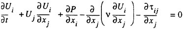
(10)
The continuity equation reads

(11)
Here, Ui represents the velocity components in the Cartesian coordinate system xi, Ρ is the pressure, ν the kin-
ematic viscosity, ρ the density and τij the Reynolds stresses.
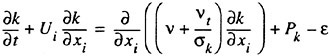
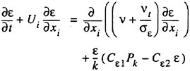
Although a number of turbulence models have been tested in the Chalmers/FLOWTECH group and elsewhere, as will be shown below, there are essentially only two models in practical use, the Baldwin-Lomax zero equation model (11) and the two equation k-ε model, where k is the turbulent kinetic energy and ε its rate of dissipation. Most methods today avoid the use of wall functions, and this calls for a special treatment of the ε-equation near the wall. A common choice is the two-layer model of Chen and Patel (12). The equations for k and ε read
(12)
(13)
where the production term Pk is defined as
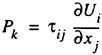
(14)
and the eddy viscosity νt is obtained from
(15)
The constants are as follows
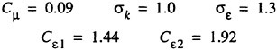
(16)
The most common boundary conditions for equations (10), (11), (12) and (13) are:
-
On the hull: Ui=k=0 (ε not needed)
-
Inflow, inner part, if there is an upstream boundary layer solution available: Ui, k and ε from the boundary layer solution
-
Inflow, outer part: Ui from potential flow solution, k and ε=small. If the calculations start in front of the hull: Ui undisturbed.
-
Outer edge: Ui from potential flow solution, or undisturbed. Sometimes symmetry conditions, k and ε=small or symmetry conditions.
-
Outflow: Most commonly Neumann condition for Ui, k and ε
-
Symmetry plane: Symmetry conditions for Ui, k and ε
-
Free surface: In most standard methods: symmetry conditions for Ui, k and ε. See section 4.2 for better free surface conditions.
A boundary condition for the pressure may be obtained either from the continuity equation or from one momentum equation.
To obtain an approximate solution to the equations, they are discretized in space and time and linearized. Numerous choices exist for solution algorithms and it is out of scope to review them here. The interested reader is referred to the proceedings of the two workshops (8), (9), where the numerical features of all participating methods are listed in detail. In general, an important capability in ship hydrodynamics is to be able to resolve thin boundary layers while taking large time steps to reach steady state, and this favours low order implicit time differencing. Spatial differencing is usually second order accurate with central differences for the diffusion term and some kind of upwind differencing for the advection term. Accuracy higher than second order has advantages, but is also less robust and more difficult to implement, especially when it comes to the boundary conditions.
3. Current capabilities
CFD is becoming an established tool in hydrodynamic design. Several methods are in routine use at shipyards, consultants and universities, and there exists a wealth of literature on various applications for different types of ships. For a review of methods and applications, see Larsson (13). In this Section an assessment will be made of the capabilities of established methods. Strong and weak points will be highlighted, and the need for the research presented in Section 4 will be explained. The discussion will address five important areas: wave pattern, wave resistance, wake/local flow, viscous resistance and propeller/hull interaction.
3.1 Wave pattern
Figure 1 presents predicted potential flow waves from two different hulls, the slender Series 60, CB=0.60 hull and the very bluff Dyne tanker, designed as a test case at the 1990 Gothenburg workshop (8). Its block coefficient is 0.85. The Froude number for the slender hull is 0.316 and for the bluff one 0.165. Wave contours along two longitudinal cuts are shown for each hull. One cut is close to the hull and the other is further out. The bow is at x=0.0 and the stern at x=1.0. Both calculations and measurements are displayed. The number of panels used in the computation was 25
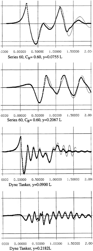
Figure 1. Wave cuts for two hulls (4)
Circles: measurement, Line: calculation
per wave length in the longitudinal direction on the surface for the Series 60 hull and 15 per wave length for the tanker. Laterally, 20 uniform panels were used for the slender hull and 15 stretched panels for the bluff one. The reason for the worse resolution of the tanker waves is the much smaller wave length, which calls for many more panels to achieve the same resolution. The number of panels followed the recommendations to the users of the SHIPFLOW code, considering available computer capacity, and the results were obtained with this software.
In general, the correspondence between calculations and measurements is quite good. For the Series 60 the wave peaks are slightly underpredicted along the hull, which indicates that the resolution is still not sufficient. Even though as many as 25 panels are used per wave length, systematic grid refinement studies (6) indicate that this is not enough to completely capture the peaks. For the cut closest to the hull an over prediction is noted in the wake. Most likely, this is caused by neglected viscous effects, i.e. the influence of the boundary layer/wake displacement effect.
The wave predictions for the tanker are surprisingly accurate, at least along the forebody, and no systematic under prediction of the peaks is noted. Considering the lower resolution this may seem to contradict the above discussion. However, most likely some breaking of the bow wave is present in this case which somewhat reduces the measured wave height. No such effects are of course considered in the calculation, so the very good correspondence may be attributed to a cancellation of (relatively small) errors. It is interesting to note what happens further aft on the hull, and particularly in the wake. The innermost cut exhibits an increasing over prediction of the wave peaks, and in the wake the predicted waves are several times larger than the measured ones. A much stronger effect of the neglected displacement effect is thus noted for this bluff hull. However, at the second cut there is practically no over prediction. Wave contours for this case show that this is due to the fact that the overpredicted stern waves have not reached the outermost cut at the end of the panelized free surface. This indicates that the waves from the rest of the hull are well predicted even at the downstream edge of the panelized surface.
The two hulls in the example represent extremes in hull bluffness and the good results of the predictions indicate that waves from the major part of the hull may be computed with good accuracy. This is utilized by ship designers in the optimization of ship forebodies and bulbs. By investigating the predicted wave pattern and wave profile, and comparing with the computed pressure distribution on the hull, experienced designers are guided in their optimization process. Good descrip-
tions of this technique are found in several papers from the Daewoo design team in Korea, see e.g. (14), and according to other users of the SHIPFLOW code, this approach is common also elsewhere. Undoubtedly, this is the best way of utilizing hydrodynamics CFD at present.
Great care is however recommended in the optimization of ship afterbodies using the above approach. As was seen in Figure 1, the real waves are modified at the stern due to viscous effects, not considered in a potential flow. When comparing two similar designs it may be tempting to assume that the ranking is unaffected by this effect, but this is not necessarily true, as was realized in a notable failure by two of the authors in the optimization of the Series 60 hull (15). Applying numerical shape optimization an optimized hull with significantly lower total resistance was developed. In later grid refinement studies this new shape was consistently better than the original hull. However, when the new hull was model tested, its resistance was slightly larger than for the original hull. A careful investigation of the possible reasons for this failure was carried out and it was found that the optimization caused a slight increase in bow wave height, while it minimized a stern wave, whose importance in reality was considerably smaller than in the computations. Further, there was a vertical shift of the boundary layer displacement thickness on the new hull, causing an increase in the wave resistance.
For high speed hulls the situation is different. If the hull has a submerged transom, the boundary layer grows much less than for a cruiser stern, where the girth length is reduced as the stern is approached and where the local convergence of streamlines may be very strong. There is thus a much smaller effect of the displacement thickness for transom stern hulls. This is, of course, provided the transom is dry. If the flow recirculates behind the transom, the problem cannot be handled by potential flow methods. Various proposals have been put forward for the boundary condition to apply at the transom edge, see (6) for review. In SHIPFLOW, the wave height at the upstream edge of each wake panel row is set equal to the transom draft at this position and this produces quite realistic waves, both behind the transom (the rooster tail wave) and laterally (5). There are thus much better prospects for optimizing the stern of a transom hull than of a displacement hull. An accurate prediction of the sinkage and trim is, however, quite important in this case, particularly at the lower range of Froude numbers for which the transom is dry. In this speed range the hydrostatic resistance, caused by the loss of hydrostatic pressure at the transom, is much larger than the hydrodynamic resistance and the former is proportional to the square of the transom draft. An interesting study of the effect of a trim change is presented in (13).
A problem attracting more and more interest is the wake wash of high speed ships. From the above discussion panel methods may appear to be a very suitable for this type of problem, but a difficulty is the large distances at which wave predictions are requested. Normally the interest is in far field waves several boat lengths away from the hull. Obviously, this is very difficult for a method that relies on a panelization of the free surface. Very limited stretching is permitted if the numerical damping of the waves is to be kept within acceptable limits. On the other hand, the non-linear free surface effects are limited to a region rather close to the hull, so predictions by a linear theory may be permitted outside this region. One possibility explored several years ago by Gadd (16) and Aanesland (17) is to match a near field method of the type described here with a far field method using Kelvin sources that automatically satisfy the linear Kelvin condition on the surface. This possibility does not seem to have been explored recently. A simple extension of the wavy surface outside the panelized region based on linear theory has been used by Hughes (18) and others.
The remedy for the stern wave problem in the case of displacement hulls is to abandon the potential flow approach and use viscous methods of the RANS type. As mentioned above, RANS methods with a free surface are becoming more and more common, but they are not at all as established as the panel methods. A major problem is resolution. Due to restrictions in computer capacity the free surface and the water layer just below the surface cannot be resolved well enough to avoid excessive damping, at least not for the low Froude number range. A more thorough discussion on free surface RANS methods will be given in Section 4.2.
3.2 Wave resistance
The wave resistance is normally computed by adding the longitudinal components of the pressure forces on all panels. This means adding of the order of 1000 contributions of different signs, which almost cancel each other. For slow ships the sum may be of the same order as one of the larger contributions. The discretization error for such ships is thus often of the same order as the resistance. In a linear method the problem may be reduced by subtracting the resistance computed for a hull without a free surface, i.e. the so called double model case. According to d’Alemberts paradox the resistance for this case (without lift) is zero, so the computed resistance may be representative of the error associated with a given panelization. Unfortunately, this technique is much more difficult to apply in a non-
linear method, where the panels normally change in the iterative process. In SHIPFLOW this is entirely true and in principle all panels change in the iterative process, when the free surface converges to its final shape. Other methods, Jensen (19), use a given panelization on the hull, which extends through the free surface and integrate only over the (part of the) panels below the surface. Although the chances of using d’Alemberťs paradox are better for these methods the correction is still approximate due to the differences in the integration close to the water surface in the wave case and the double model case.
Better corrections for the discretization error can thus be devised for linear methods, but they are still inferior to the non-linear ones due to the linearization. As explained in Section 2, the linearization means two types of approximation: a neglect of the non-linear terms in the boundary conditions and a transfer of the conditions to the undisturbed free surface. Both contribute to inaccuracies. As shown by Raven (6) the approximation of the equations leads to a flow of energy through the surface. This may either increase or decrease the resistance. The erroneous location of the conditions normally leads to a reduction in resistance, since the positive contribution to the resistance from the bow wave above the undisturbed free surface is neglected, while a non-existing suction force below this surface is included. At the stern the effects are reversed, but normally much smaller. Very frequently, negative values of the wave resistance are found for linear methods and low Froude numbers.
There are thus several reasons why resistance calculations are inaccurate in the low speed range. A negative wave resistance is seldom found for non-linear methods, but the accuracy in the predicted resistance is still unacceptably low for slow ships, i.e. at least up to a Froude number of 0.20. In the intermediate speed range the prospects are better, since the wave resistance at these speeds is much larger than the discretization error. The most accurate calculations of the wave resistance are found for semi-planing hulls, from the Froude number where the flow clears the transom, around 0.35, up to about 1.0. Above this Froude number non-linear effects like spray, not accounted for, become too important.
One way to improve the wave resistance prediction is to derive an empirical correction to the computed value. This may be accomplished by comparing large sets of measurements and calculations for a specific type of ships. At SSPA this technique is used for round bilge semi-planing hulls and the Technical University of Berlin (20) reports on successful corrections to slender cargo ships. It is very unlikely, however, that a similar correction can be found for slow ships.
A more scientific way of improving the resistance prediction is to abandon the pressure integration technique and obtain the resistance from the computed waves. Since these are rather well predicted a more accurate resistance might be envisaged. Some attempts to follow this track have been made recently. A longitudinal cut method was tested by two Chalmers students in 1995 with promising results, and this idea was pursued by two of the authors in 1997 (15). More work is planned to optimize the technique, but there is no doubt that an improvement relative to the pressure integration technique is possible. A very interesting alternative is presently being investigated at MARIN (21), where a transverse cut technique is being developed. In principle, this technique is less approximate, since no truncation of the cut within the wave system needs to be done. While a transverse cut may cover the whole Kelvin wedge, a longitudinal cut must be truncated somewhere and analytically extended to infinity.
3.3 Wake/local flow
In Figure 2 a comparison is made between the predicted and measured wake contours of a very bluff hull, the Dyne tanker, designed for the 1990 workshop (8). The results are from the workshop, and are thus quite old, but they are still typical of most methods using standard turbulence models.
As can be seen in the figure, the contours in the propeller disk are not well predicted. While the computed contours are quite smooth, the measured ones exhibit an island and a quite pronounced “hook”. During the nineties much of the research in viscous flow CFD has been directed towards improving the ability to predict these features.
On closer inspection it turns out that the wake hooks, which are present for large classes of ships, are caused by the bilge vortices (one on each side), generated at the bilge and hitting the propeller plane inside the propeller disk. An accurate calculation of these vortices is thus important for the prediction of the hooks. This calls for a more advanced turbulence modelling than what was available in the early nineties. At the 1990 workshop the only models used were zero equation models of the Baldwin-Lomax type and the two equation k-ε model. The latter is still the most widely used one and is normally available in commercial RANS codes. Therefore, good wake contours cannot be expected using standard codes, at least for full ship forms. Very slender hulls, on the other hand, do not normally have pronounced bilge vortices, and quite accurate wake contours can be predicted, see for instance Zhang et al (22). It should be pointed out that, although the details of the contours are not well captured for the bluff hull, integrated quantities are better.
The radial variation of the circumferentially averaged wake, important for designing the pitch distribution, is thus better than the contours but not accurate enough for design purposes (23). The wake fraction, on the other hand, can normally be obtained with sufficient accuracy (22), (23), (24).
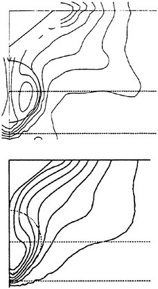
Figure 2. HSVA Tanker, wake contours in the propeller plane. Outermost contour: 0.9, interval: 0.1. Top: measurement. Bottom: calculations (8).
Since the wake contours in the propeller plane are insufficiently accurate, local viscous flow predictions may be questioned. Certainly, if predictions are requested as far aft as the propeller great care must be exercised when interpreting the results. However, local flow directions are often requested elsewhere, for the positioning of bilge keels, brackets and fins. Experience shows that such predictions are mostly sufficiently accurate for design purposes. As pointed out above, transom stern ships, have a relatively thin boundary layer even close to the stern, and bilge vortices are seldom a problem. For such hulls very good viscous flow predictions are possible, an important advantage, since these hulls often have brackets, whose direction can be optimized.
To improve the situation, more accurate turbulence models are required and several predictions have been reported where considerably improved results are demonstrated. This development will be discussed in Section 4.3.
3.4 Viscous resistance
The inability to compute the details of the wake flow certainly has some effect on the accuracy of the prediction also of the viscous resistance. However, the resistance is an integrated value, so just as in the case of the wake fraction, the details of the flow do not necessarily have to be very accurate to obtain a value of engineering interest. Therefore, existing RANS solvers should be capable of predicting the viscous resistance accurately enough for ranking purposes, provided certain conditions are satisfied. Where many methods fail is the grid quality. In particular, an accurate representation of the hull shape at the ends is important. Many grid generators produce a staircase-like hull shape at the stern contour, with very distorted numerical cells. Since this is an area of large importance for the resistance, both the erroneous direction of the normal to the hull surface and the inaccurate pressure contribute to an unrealistic pressure drag. For this to be computed accurately it is also important to have a sufficient number of grid points in the direction normal to the hull to resolve the pressure variation across the boundary layer. The frictional resistance, on the other hand, relies on an accurate prediction of the flow in the inner part of the boundary layer. The innermost points of the grid must thus satisfy given requirements for y+, be it a wall function method or a method using the no-slip condition. Grid dependence studies are certainly important in all CFD work, but especially in resistance prediction.
The viscous resistance was provided by eight methods at the 1994 workshop (9). Three were seriously in error and three predicted the resistance, as well as the split between the pressure and frictional contributions, quite well. There was no discernable advantage of the k-ε model as compared to the Baldwin-Lomax model and the methods were in most respects quite similar, so the different performance must be due to numerical details, most probably related to the grid. This conjecture is substantiated by the fact that careful grid refinement studies have been reported elsewhere for two of the three best methods, see Ju and Patel (25), and Ishikawa (26). In both papers successful rankings of hull afterbodies are reported. Streckwall (27) also reports on successful rankings and in a recent paper Masuda and Kasahara (24) present interesting calculations of the form factor for 20 hulls using the NICE code (28). The latter introduce a correlation between the predicted and measured form factors, and using this correlation, the error in the predicted values are within 2% for 18 out of the 20 hulls. As mentioned above, this is an good way of increasing the engineering value of CFD. It should be mentioned that a similar correlation was developed for the wake fraction.
3.5 Propeller/hull interaction
Already in 1977 Schetz and Favin proposed an actuator disk approach to introduce propeller effects in RANS methods. By applying body forces to the numerical cells in the propeller disk the flow may be accelerated in the same way as by a propeller with an infinite number of blades, producing the same thrust and torque. This approach was further refined and improved by Stern and his co-workers in Iowa (29), and in the Chalmers group by Zhang (22). More recently the method has been applied to design problems at the University of Athens (30). A somewhat simpler approach is to apply a pressure jump in the propeller disk, see Streckwall (27).
An actuator disk is now included in the SHIPFLOW code, where the body forces are computed by a lifting line propeller analysis method, run interactively with the RANS solver. Using the velocity computed in each numerical cell within the propeller disk, the lifting line program computes the circulation and thereby also the axial and tangential body forces, which are returned to the flow solver in an iterative process. Strong under relaxation is required to introduce the body forces, but the iterations are included in the normal pressure/ velocity iterations, so the computer effort is not much increased Since the code can be run with a propeller only, corresponding to an open water test, the propulsive factors can be computed.
Although the actuator disk has been available in SHIPFLOW for a couple of years it does not seem to have been much used. It is therefore difficult to assess the accuracy of the computed propulsive factors. Zhang’s own calculations (22), as well as more recent work in a Master’s thesis indicate that the thrust deduction can be obtained with good accuracy even for high speed hulls, where a large part of the thrust deduction comes from trim changes. The effective wake and the relative rotative efficiency also seem to be reasonable. The actuator disk approach should be further evaluated and used by the designers. It seems to be a useful tool for power prediction (of course with the limitations of the resistance calculation). For more accurate predictions of blade flows and pressure fluctuations the more advanced methods presented in Section 4.4 will be required.
4. Present research
As explained above, the most advanced potential flow methods have now reached a state where the major obstacle for further improvement is the inherent neglect of viscosity, and the efforts to fine tune available methods have been covered already in Section 3. Therefore, the present section will only cover research in the RANS area. The work presented may be expected to yield improvements in existing solvers in the relatively near future, say five years, while the more long range perspectives will be discussed in Section 5. Although reference will be given to research elsewhere, the emphasis will be on the work in the Chalmers/FLOWTECH group. Four areas will be covered: grid generation, free surface boundary conditions, turbulence modelling and propeller blade flows.
4.1 Grid generation
The ship hull is normally a smooth surface and the flow domain surrounding the hull may rather easily be transformed into a rectangular box, in which the computations are performed. Ship flows are therefore good candidates for single block structured grids, and so far the vast majority of ship flow methods employ grids of this kind. In the 1990 and 1994 workshops (8), (9) all methods used single block structured grids. There are, however, several reasons for introducing more advanced gridding. Although the hull itself is smooth, it always has appendages of different kinds. These are normally neglected, but for more advanced calculations the rudder, possible shafts and shaft brackets, bilge keels, fins, etc. have to be taken into account. A single block grid necessarily has to include singular points or lines in front of and behind the hull and this calls for special treatment in the solver. Further, a large number of grid points are normally wasted in regions where they are not needed in structured single block grids and, as pointed out above, it is difficult to obtain a high grid quality close to the ends of the hull.
For these reasons there is a growing interest in developing methods based on less restrictive gridding techniques. Little interest has however, been shown in completely unstructured grids, common in structural mechanics. Such techniques offer great flexibility, but impose more work on the solver, which has to take care of the connectivity information and has to deal with large sparse matrices. It is also more complicated to develop higher order schemes and multi-grid convergence acceleration techniques. Completely unstructured grids are also unsuitable for boundary layers at high Reynolds numbers, where extremely large gradients are experienced in the direction normal to the surface. These disadvantages are often offset by the advantage in flexibility for general purpose CFD applications, where unstructured grids may be an alternative, but in hydrodynamics this does not seem to be the case and only a few calculations with unstructured grids have been reported, see Hino (31) and a recent paper by Yang and Loehner (32).
Instead, the recent interest among hydrodynamicists has been directed towards multi-block methods,
where the structure is maintained within each block. Not surprisingly, this development started in submarine hydrodynamics, where appendages play an important part. Standard multi-block techniques for submarines are reported by Sung et al (33), McDonald and Whitfield (34) and Bull (35). Other applications are presented by Cowles and Martinelli (36) and Beddhu et al (37). The traditional multiblock techniques offer more flexibility than single block grids, but they are still restricted due to the need for matching at the common boundaries of adjacent blocks. A more modern approach is to let the grids overlap without any restrictions on continuity of grid lines. This technique, known in the United States as the Chimera technique, has become a useful tool in many engineering branches, see the 1st–4th Symposia on Overset Composite Grid & Solution Technology. (The 4th one to be held at the Army Research Laboratory, Aberdeen, Maryland, USA 23–25 September 1998). Recent applications of overlapping grids in hydrodynamics include Weems et al (38), Lin et al (39) and Masuko (40).
In the Chalmers/FLOWTECH group a new 3-D overlapping grid generator CHALMESH has been developed by Dr. Anders Petersson, based on his earlier 2-D code XCOG (41). The new code has an efficient user interface and seems more robust than other grid generators of this kind. Based on overlapping surface grids, which have to be provided for general cases, overlapping volume grids are grown hyperbolically out from the surface. The body-fitted grids may be embedded in one or more background grids, which may be curvi-linear or Cartesian. Holes are automatically cut out and the necessary overlap is ensured. Interpolation weights are computed and saved for all interpolation points at the edge of each grid. To avoid mismatch, special techniques are used to handle the interpolation between the extremely thin cells close to boundaries where the no-slip condition is to be applied. CHALMESH is reported in (42), and the code is available free of charge for research purposes on the Internet under the address: http://www.na.chalmers.se/%7Eandersp/chalmesh/chalmesh.html. It is presently used at different departments at several universities in Sweden and the USA.
Figure 3 shows the grid generated around a three-bladed propeller. Only surface grids are shown for two of the blades, while a cut through the body-fitted grids is shown for the third blade. It is seen that there are three grids on each blade, one on each side and one wrapped around the edge. These grids are embedded in a background cylindrical grid. By arranging the grids in this way quite orthogonal grid lines may be obtained. On ship hulls typically a few grid patches are wrapped around the stern, after which a
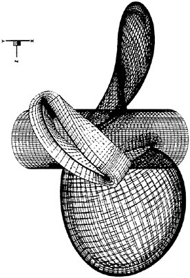
Figure 3. The grid around a 3-bladed propeller. Body fitted volume grid shown on one blade only.
couple of rectangular grids are attached. All these are embedded into a background cylindrical grid. The rectangular grids are added to remove the line singularity of the background grid.
A new RANS method for overlapping grids has been developed within the group, mainly by Björn Regnström. Finite difference discretization is used and the discretized equations are solved implicitly for all blocks, i.e. the matrix contains equations for all points including interpolation points. To keep the discretization stencil as small as possible, central differencing is used for all terms. Alternatively, a mix of second order central and first order upwind discretization may be used for the convective terms. To stabilize the solution if central differences are used, artificial dissipation is added. The variables are collocated and Rhie-Chow interpolation is used to avoid pressure fluctuations in the SIMPLE pressure/velocity updating scheme. As will be seen below, the free surface is treated in a special way and a range of turbulence models are available. By the time of writing, laminar flow calculations have been carried out for the propeller of Figure 3, and the first turbulent results have been obtained for a ship hull. The results indicate that the overlapping algorithm works as expected, but some other fine tuning of the method is required before it can be used on a regular basis.
4.2 Free surface boundary conditions
As mentioned above, the most important result of the 1994 workshop (9) was the breakthrough of the
free surface RANS methods. No less than 10 methods featured this capability. The technique was not new, however. The Marker and Cell (MAC) method had been available for 30 years and the Volume of Fluid (VOF) method for more than 10, but they had mainly been applied to internal flow problems, such as sloshing. In ship hydrodynamics the first references are from the mid-eighties, when Miyata et al introduced their version of the MAC method called TUMMAC (43). A large number of references to subsequent developments in different groups are available and may be found in Larsson (13). They will not be repeated here. See however Miyata (44) for an overview of the impressive developments at the Tokyo University. Recent references, not in (13), include Yang and Loehner (Euler solution) (32), Beddhu et al (37) and Haussling et al (45). The latter is especially interesting, since it deals with the difficult transom stern problem.
Extensions into other areas of hydrodynamics are presented in the papers by Rhee and Stern (46), Campana et al (47) and Ohmori et al (48). While Rhee and Stern compute the wave diffraction from a fixed hull subjected to an approaching wave train, the others consider the side force and turning moment of a hull at a yaw angle.
In general, predicted wave profiles along the surface of the hull agree well with measurements, while the wave height away from the hull is consistently underpredicted. This is true especially for the diverging waves, which are not well captured even at high Froude numbers (above 0.3). In the low Froude number range (below 0.2) all waves are damped out at a relatively short distance from the hull. The reason for this is obviously bad resolution. To investigate the requirements on grid resolution a Korean visiting scientist in the Chalmers/FLOWTECH group, Dr. Kang, carried out systematic grid refinement studies for the waves generated by a submerged airfoil (49). A 2-D free surface RANS code was used and great care was taken to reduce the numerical damping on the surface. It was found that approximately 50 points per wave length were needed to preserve the waves.
In a 3-D case the diverging waves have the shortest wave lengths, and as pointed out by Mori and Hinatsu (50), about five times denser grids are required in the transverse direction as compared to the longitudinal direction to really capture these waves. This means that the requirements on the number of grid points become prohibitive on today’s computers. For instance, at a Froude number of 0.15, where the fundamental wave length is about 1/7 of the hull length, approximately 106 grid points would be required on the wavy surface. Now, the dense grid could probably be concentrated in a layer relatively close to the surface, but to maintain the density in the vertical direction very near the surface the total number of points would be somewhere in the range 107–108.
Since the wave length is proportional to the square of the Froude number, the number of points on the surface would be inversely proportional to the fourth power of the Froude number, if the extension of the gridded part of the surface was kept constant. Now, the gridded part normally increases somewhat with wave length, but normally much less than linearly. Assuming that the required number of points in the vertical direction is independent of the wave length and the free surface is unchanged, the total number of points at a Froude number of 0.3 would be one order of magnitude smaller than at 0.15, i.e. in the range 106–107. No predictions presented so far have been anywhere near this number. The largest cases presented have had a total number of grid points around 106, while the number of points on the surface has been of the order of 104. This is why the Kelvin wave pattern is not obtained. It should be pointed out that panel methods seem to be able to predict very detailed wave patterns even at the lowest Froude numbers using less than 104 panels on the surface. The inability of the RANS methods to capture the waves is, of course, only a temporary problem. As will be seen below there are good prospects for increasing the number of points on the surface considerably within the not too distant future. Further, a good Kelvin wave system might not be needed for other predictions of interest, such as wave resistance, sinkage and trim, side forces and other local phenomena.
In the first free surface RANS methods of the MAC and VOF types the grid was kept fixed and the free surface tracked in the grid at every time step. This technique has been abandoned in most recent methods (a notable exception is TUMMAC), where the grid is fitted to the free surface and deformed as the waves grow with time. As pointed out in Section 2, there are two boundary conditions on the surface, the kinematic one (4) and the dynamic one. (5) represents an inviscid approximation of the latter. The exact dynamic condition expresses continuity of stresses across the surface, i.e
(17)
where the star represents values in the air.
This condition is, however rarely used. With few exceptions (Alessandrini and Delommeau (51)) the inviscid approximation is adopted, i.e. the pressure is assumed constant and set to zero. Bernoulli’s theorem cannot be used, however, so (17) may now be written
as follows
(18)
neglecting surface tension.
In most methods (18) is used as a condition for the pressure in each time step, while an unsteady version of (4) is used to update the location of the surface (and the grid) after each step. The advantage of the moving grid method is that the interface is sharp, so that grid point may be concentrated near the surface.
Another technique is under development in the Chalmers/FLOWTECH group, Vogt (52), (53). Like in the earlier methods, the grid is again kept fixed, and the surface tracked at every time step. The tracking is however different from the previous ones and based on the so called level set technique.
The computational domain includes both the water and part of the air above the surface. Initially the flow is at rest and a scalar “level set” function ![]() is defined in the whole domain by the distance from the flat free surface, positive downwards and negative upwards. After solving the flow equations in every time step, a differential equation for
is defined in the whole domain by the distance from the flat free surface, positive downwards and negative upwards. After solving the flow equations in every time step, a differential equation for ![]() is solved
is solved
(19)
i.e. the substantial derivative of ![]() is equal to zero. This means that every fluid particle is assigned an invariant value of
is equal to zero. This means that every fluid particle is assigned an invariant value of ![]() . The kinematic boundary condition (4) on the free surface states that the normal velocity on the surface is zero, which means that a particle once on the surface will stay there forever. Since
. The kinematic boundary condition (4) on the free surface states that the normal velocity on the surface is zero, which means that a particle once on the surface will stay there forever. Since ![]() was initially zero on the free surface, that surface will at any later time correspond to the surface
was initially zero on the free surface, that surface will at any later time correspond to the surface ![]() . It should be mentioned that a reinitialisation of the level set function is required after a few time steps, when lines of constant
. It should be mentioned that a reinitialisation of the level set function is required after a few time steps, when lines of constant ![]() may get very distorted, particularly in the air.
may get very distorted, particularly in the air.
Since the flow equations are solved in two different fluids simultaneously, physical parameters have to change at the interface. For numerical reasons a stepwise change is not possible, so a smooth variation in a thin layer at the surface is required. The necessary thickness and number of grid points of this layer, as well as other numerical parameters have been investigated by Vogt (52) and it was shown that the level set technique is an interesting alternative to the conventional moving grid methods.
A major advantage of the level set technique is that complex wave shapes may be represented. There are no restrictions with respect to overturning waves or even changes in topology, such as wave plunging or drop formation (53). Another advantage is that updates
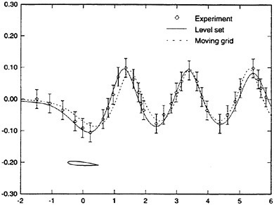
Figure 4. Comparison between level set and moving grid method. Wave from submerged wing.
of the grid and its geometrical quantities are not needed, as in the moving grid method. The technique is also robust and straightforward to implement in computer codes. In Figure 4 a comparison is made between results of the level set technique and a conventional moving grid solution for the free surface above a submerged wing. Both methods predict the wave within the experimental accuracy.
One disadvantage of the level set technique is that the flow has to be computed also in the air, where it might not be requested. The somewhat diffuse interface is another disadvantage, which increases the difficulty of concentrating grid points exactly where they are needed. The latter problem may be alleviated using the overlapping grid technique in a thin layer around the interface. Based on an extensive investigation in 2-D, Vogt (53) concluded that the level set technique is slightly more time consuming than the moving grid technique for comparable accuracy. The difference is small, however.
In conclusion, there are different free surface techniques available in RANS methods. None of them is presently capable of computing an accurate Kelvin wave pattern due to resolution problems, but this problem will be solved as the computer power increases.
4.3 Turbulence modelling
An interesting clue in the search for better stern flow prediction methods was presented by Deng et al (54) in 1993. By an ad hoc reduction of the predicted eddy viscosity in the bilge vortex a considerable improvement in the wake contours of the HSVA tanker was noted. This indicated that the major weakness of contemporary RANS methods in their ability to predict
the wake details was the inaccurate turbulence modelling. In retrospect, this is not surprising, since the only models used so far were the zero equation Baldwin-Lomax model and the two equation k-ε model, both based on the Boussinesq assumption of a scalar eddy viscosity and with no consideration of extra rates of strain, such as rotation.
The results by Deng et al (54) inspired several groups to look into more complex turbulence models, and at the 1994 workshop (9) two methods incorporated full Reynolds stress models. Considerable improvements were noted, especially for the method by Sotiropoulos and Patel, and in a later paper (55) more results were presented, which strongly supported the use of their Reynolds stress model. One result is shown in Figure 5 where the prediction of the wake contours in the propeller plane of the HSVA hull is shown. Note the improvement relative to Figure 2!
The incorporation of a Reynolds stress model is not, however, a straightforward task, as pointed out by Deng and Vissoneau (56), since the momentum equations represent a subtle balance between terms of different origin and where pressure and shear stress gradients may be equally important. They therefore proposed a modification to the pressure/velocity algorithm, in which the turbulent stresses were included in the iterative process, and this stabilized the solution.
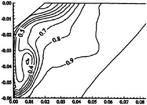
Figure 5. HSVA Tanker wake contours computed by a Reynolds Stress Model
Since a Reynolds stress model includes six more transport equations as compared to the k-ε model, the computational effort increases considerably, even if the stability problem may be solved. Therefore it is of great interest to try to find simpler models with the requested capabilities. In an extensive investigation in the Chalmers/FLOWTECH group Svennberg investigates a range of turbulence models for several cases of relevance to the ship stern flow. The first report (57) includes a test of eight models ranging from the k-ε model to a full Reynolds stress model and the test case is a free vortex in a wind tunnel. Figure 6 shows the computed results at a downstream station for five of the most interesting models: the standard k-ε model (KE), the k-ω model according to Wilcox (KO), an algebraic stress model due to Gatski and Speziale with a second order constitutive relation (GS), a similar model due to Launder with a third order relation (LAU) and the Launder-Shima Reynolds stress model (RSM). Convincing results are shown for the RSM, while the KE and KO models smear out the velocity variations in both figures. A very interesting possibility is, however,
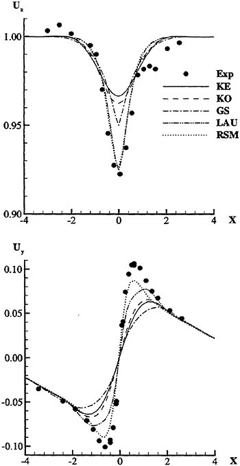
Figure 6. Velocity distribution in a free vortex. Top: Axial velocity. Bottom: Tangential velocity.
the LAU model, which is almost as accurate as the RSM and without its disadvantages. In the LAU model the Reynolds stresses are obtained from the strain and vorticity tensors
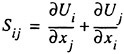
(20)
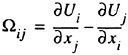
(21)
as follows
(22)
where δij is the Kronecker delta and aij is the anisotropic stress-strain relation that takes the form:
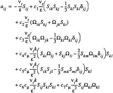
(23)
where c1–c7 are constants. There is thus a strong influence of rotation and all Reynolds stress components are computed individually.
Some results for Svennberg’s second test case, two counter rotating vortices in a flat plate boundary layer, have been presented recently in (58) and the advantage of the LAU model as compared to the KE model is confirmed. The final calculations including a full tanker hull will be completed shortly.
One more result from the first test should be mentioned. Although the RSM was the best for the predictions of Figure 6 it was in fact inferior to the KE model for a case where the vortex centre included a strong jet. This is not an interesting case for the stern flow prediction, but it may be of interest in connection with propeller modelling. Perhaps the most important conclusion from this is that the RSM is also a model with weak points, in this case the linear pressure-strain relationship, which is not suitable for jet cases, see Wilcox (59).
The search for models with the most important capabilities, but without the disadvantages of the Reynolds stress models has led to some interesting results in Japan recently. First some simple modifications of an ad hoc nature have been applied to the Baldwin-Lomax model, Tahara and Himeno (60), Kodama (61). A pressure gradient correction applied to the outer eddy viscosity has been derived based on experimental data from axisymmetric bodies. Further, the eddy viscosity is reduced based on the angle between the velocity and vorticity vectors and the vorticity is taken to be the component at right angles to the wall shear stress. The modifications have resulted in considerable improvements in the stern flow prediction for the test cases shown in the papers (24), (60), (61).
A modification of a more fundamental nature is the change of the production term in the ε-equation proposed by Okimoto et al (62). The new term, which is derived from first principles, includes the vorticity vector and could be of importance when predicting vortical flows. So far the model has only been applied to a generic case, and it has only been reported in Japanese, but its further development and testing will be of interest.
4.4 Propeller flows
During the nineties there has been a strong development in the prediction of propeller blade flows using RANS methods. This work was pioneered by Stern’s group in Iowa, which already in 1990 presented calculations for a propeller with an infinite pitch (63) and in several later papers predictions for more realistic configurations have been presented, see e.g. (64). Other investigators are Oh and Kang (65), Uto (66), Stanier (67), Sanchez-Caja (68), Abdel-Maksoud et al (69) and Mc Donald and Whitfield (34). In recent workshop on propeller CFD organized by the 22nd ITTC Propulsion Committee (5–6 April 1998 in Grenoble, France) eight different methods had been applied to the test case provided.
Most methods use structured multi-block grids, but the number of grid points vary from around 105 to more than 106. Standard turbulence models are used, either Baldwin-Lomax or some version of the k-ε model. The solvers are of different types, either finite volume or finite difference.
A surprising result of most recent calculations, in particular those presented at the workshop, is the very high accuracy in the prediction of the propeller characteristics. Over a range of advance ratios many methods predict the thrust coefficient within a few per cent of the measured one and the torque is not much worse. The result is surprising, since the presented pressure distributions are generally not in good agreement with experimental data, particularly at he inner radii, where the pressure is mostly under predicted. The
lift may still be reasonable, however, since the under prediction occurs on both sides of the blade. Further out, better correspondence with the data is obtained.
The most advanced calculations of this kind are the unsteady RANS predictions by Mc Donald and Whitfield (34) for the operating propeller behind a submarine and by Abdel-Maksoud et al (69) for the self propelled Series 60 hull. Such calculations require moving grid facilities, where the propeller grid is fixed to the blades and rotates inside the hull grid.
4.5 Full scale
The ultimate goal of ship hydrodynamics CFD is of course to predict the full scale case. If this were possible, the uncertainty in the model-ship extrapolation procedure, inevitable in a towing tank, would be avoided. Unfortunately, the application of CFD at very high Reynolds numbers is not straightforward. This is both for numerical and physical reasons. The general problem is that the ratio of the smallest to the largest scales of the flow decreases with Reynolds number. Numerically, this means that more grid points are required to obtain a given resolution and physically the nature of turbulence changes, which means that turbulence models developed at low Reynolds numbers might not be valid.
For RANS methods one important scale is the viscous length scale l+=ν/uτ, where uτ is the friction velocity defined as (τw/ρ)1/2 and τw is the wall shear stress. l+ is typically two orders of magnitude smaller, relative to the hull length, at full scale as compared to model scale. Fortunately, in a Reynolds-averaged method the scale is only important in the direction normal to the hull, where it determines the velocity distribution in the inner part of the boundary layer (neglecting surface roughness effects). To obtain sufficient resolution two orders of magnitude more grid points would thus be required, or perhaps somewhat less, if larger stretching of the grid is applied. The problem is that this gives rise to extremely elongated numerical cells near the hull surface, where the first grid point must be within y+=1. y is the distance from the surface and y+=y/l+. A typical longitudinal step size is 10−2 L, where L is the hull length, while the step size in the normal direction corresponding to y+=1 is of the order of 10−8 L. The aspect ratio of the first cell is thus 106. This causes most solvers to break down, due to bad conditioning of the system of equations. Some methods are, however, surprisingly robust. Eca and Hoekstra (70), managed to compute full scale Reynolds number cases even with the first grid point at y+=0.1. The reason for the robustness of their method, PARNASSOS, is not clear. Watson and Bull (71) carried out calculations for a series of Reynolds numbers using the commercial flow solver CFX. For the three lowest Reynolds numbers, ranging from 5×10⁶ to 5×10⁸ they kept the first grid point at y+=1, while the calculations at the highest Reynolds number, 109, had to be carried out with the 5×10⁸ grid. Three interesting flat plate investigations using CFD up to very high Reynolds numbers have also been reported recently, Ishikawa (72), Dolphin (see Patel (73)) and Schweighofer (74). They will be further discussed below.
One remedy for the high aspect ratio problem is to use wall functions for representing the flow close to the surface. The first grid point may then be placed two orders of magnitude further out, which gives an aspect ratio of the first cell of the order of 104 at full scale, about the same as for methods without wall functions at model scale. This fact was utilized by Sames (75), who used the same grid at both scales, with wall functions at the high Reynolds number and without at model scale. Other full scale predictions using wall functions are those of Larsson et al (8) and Ju and Patel (76) As pointed out by Patel (73) there are good prospects for using wall functions at high Reynolds numbers, since experimental data indicate that the wall law extends to much higher values of y+ at full scale than at model scale. I fact, even the same grid might be used. However, the use of wall functions is presently abandoned by most CFD developers, since the analytical representation of the flow is not sufficiently accurate in 3-D flows with strong pressure gradients, particularly near separation.
The physical problem with high Reynolds numbers is the lack of experimental data to validate turbulence models, which have all been developed based on empirical data at moderate Reynolds numbers. Some scattered data exist for ship stern flow, but the amount of data is too small even for the validation of the mean velocities. Mostly only a small part of the propeller disk is covered. More useful are the databases obtained for the high Reynolds number flow around an axisymmetric body by Coder (77) and in the “super pipe” experiment at Princeton University, see Patel (73). Calculations for the former case were carried out by Ju and Patel (76) using wall functions and the k-ε turbulence model up to a Reynolds number of 109 and the agreement with the data was quite good at the highest Reynolds numbers. Good results at the highest Reynolds numbers were obtained also for the super pipe case using the two layer k-ε model described in Section 2 and the k-ω model by Wilcox (59). The latter model was, however, less accurate at lower Reynolds numbers. In this case the highest Reynolds number was 3× 10⁸, based on the pipe diameter, which corresponds to an order of magnitude higher Reynolds number based on body length for a flow around a body.
As mentioned above, three different flat plate calculations at varying Reynolds numbers have been reported recently. The most comprehensive one seems to be that of Schweighofer (74). Four different turbulence models were tested in the Reynolds number range 5×10⁶–1.3×10⁹, namely the Cebeci-Smith and Baldwin Lomax algebraic models, Menter’s k-ω/ε shear stress transport (SST) model and Chien’s low Reynolds number k-ε model. The CFD method was the well validated FINFLO solver and careful grid dependence studies were performed. Unfortunately, the only comparison that can be made with data is for the integrated skin friction coefficient, which can be compared with generally accepted formulas, such as the ITTC—57 line. It turned out that all models but Chien’s predicted the ITTC skin friction very well at the highest Froude number. A slight under prediction of less than 1% was obtained. However, at the lowest Froude number the under prediction was about 7–8% for all models. In fact, a better correspondence over the whole Reynolds number range was obtained with the Engineering Science Database, which is closer to the Schoenherr line. Schweighofer’s results are consistent with those by Ishikawa (72) who used the Baldwin-Lomax model and found a very good correspondence with the ITTC line at the highest Reynolds number (difference less than 0.5%), while the under prediction at the lowest Reynolds number was about 9%. The third investigation, by Dolphin (see Patel (73)) is consistent with the other two in that the slope of the friction line is smaller than the ITTC line, but the computed values are somewhat higher in the whole Reynolds number range. This results in an over prediction at the highest Reynolds number by 11%. Dolphin used the Baldwin-Lomax model and the reason for his larger values cannot be found without access to the original report (an MSc thesis).
In general, the prospects for full scale RANS predictions are good. Methods which can handle the numerical problems are already available and existing turbulence models do not seem to be seriously in error at the higher Reynolds number. The strong stretching of the grids used so far is likely to reduce the numerical accuracy, but this is a temporary problem which will be alleviated as the power of computer increases. A problem not discussed is the surface roughness, which becomes more important at higher Reynolds numbers (see Patel (73)), but existing methods to include this effect should be good for estimates also at full scale.
5. Outlook
The developments described in Section 4 will lead to considerable improvements in the capability of CFD to predict ship flows both at model scale and full scale. The perspective is here relatively short, say 5 years. In the present Section the long term possibilities will be discussed. Naturally, this will be more speculative.
There is a strong link between the developments of computer capacity and CFD, and to predict future capabilities in ship flow computation some forecast must be made of the increase in computer power. As is well known the increase in processor speed has followed “Moore’s law” during the past 30 years. Moore’s law states that the speed is doubled every 18 months, or equivalently, there is a speed-up of one order of magnitude every 5 years. In a recent speech Gordon Moore himself (78) predicted this trend to continue “at least for several years”. Other sources (79) even claim an acceleration in the development rate. Further, a development towards multiple processors may be envisaged and already today the world’s fastest computers rely on massive parallelization. In December 1996, the Intel Corporation demonstrated a machine with an achieved computing speed of more than 1012 flops (1 teraflop, Tflop) using more than 7000 Pentium Pro processors. This development is predicted to accelerate and the current goal is to reach a speed of 1015 flops (1 petaflop, Pflop) before 2010, using of the order of 105–106 processors, see Bailey et al (80) or Keyes et al (79). High end computers are thus projected to increase the speed by a factor of 103 in the next 12 years and, in view of the above, a similar speed-up seems feasible also for more generally available computers, equipped with several processors.
Most CFD calculations today are run at high end workstations, which have an achieved speed of around 108 flops (100 Mflops). Good super computers are about 100 times faster. With the projected thousandfold increase in speed the super computer will be 105 times faster than today’s workstations. To make use of the increased speeds, numerical algorithms must be developed to meet the requirements on massively parallel processing, but according to Keyes et al (79) CFD methods are among the most suitable ones for this purpose. Price is another issue, but again past experience shows that the performance/price ratio increases even faster than performance itself. Neither should the increased storage requirements pose any problems (79).
What, then, can be achieved with these powerful computers? For a good multigrid method, the computer effort per time step is proportional to the number of grid points. This means that even on regular workstations the number of grid points could increase from the present level between 105 and 106 to about 108. With this increase in grid density, according to Section
4.2, there will be no problems resolving the free surface flow. Neither will there be a problem resolving the viscous full scale flow in a RANS method with the same resolution as presently at model scale. Accurate full scale RANS calculations with a free surface thus seem feasible.
Even more exciting are the prospects for less approximate solutions of the Navier-Stokes equations. Large eddy simulations (LES) should be more exact than RANS, since only the smaller eddies, which are more universal, i.e. less dependant on the boundary conditions, need to be modelled. Ultimately, even direct numerical solutions (DNS) may be feasible. In a recent paper one of the authors (Larsson (23)) estimated the computational effort required for LES and DNS solutions at model and full scale Reynolds numbers. The estimate was based on the assumption that the smallest scale of the flow, the Kolmogorov turbulence scale, should be resolved. Following Wilcox (59) and assuming that the boundary layer thickness could be set equal to half the channel height, experience from channel flow calculations could be utilized The estimate took into account the number of grid points as well as the number of time steps required, but it did not consider the lateral extension of the hull surface. Considering this, the effort for model scale LES will be 104–105 times that of a RANS solution today. For DNS the increase will be 106–107 times. LES is thus likely to be possible before 2010 on super computers. Within another decade model scale LES might be possible on workstations and DNS on super computers. At that stage the accuracy of the CFD predictions will have passed that of the towing tank.
6. Conclusions
In this review the present status of CFD in ship hydrodynamics has been assessed. Ongoing research has been reviewed and the short term benefits of the research has been evaluated. Long term developments relying on increases in computer capacity have been outlined. The main conclusions are:
-
At present, the most useful CFD results are offered by the potential flow panel methods which are used extensively for the optimization of hull shapes. Optimization of cruiser stern shapes should be avoided, however.
-
The optimization is normally based on the predicted waves and hull pressure distribution. Wave resistance coefficients may be used as well at higher speed but should not, at present, be trusted at low speeds (below Fn=0.2, say).
-
RANS methods can predict integrated quantities of the wake reasonably well, while the details cannot be obtained accurately.
-
The viscous resistance obtained by RANS methods is accurate enough for ranking purposes, provided care is exercised in the generation of the grid, particularly at the hull ends.
-
The body force approach is common for representing the propeller and many methods are capable of predicting the propeller/hull interaction.
-
Great efforts are being made to improve the grid generation and one interesting approach is the Chimera technique, which facilitates the inclusion of appendages.
-
Many free surface RANS methods are now available. The normally predict the hull wave profile quite well, but cannot predict the Kelvin wave pattern due to insufficient resolution. This problem will be removed thanks to the increase in computer power.
-
Turbulence modelling is the key issue in the prediction of the wake details. Full Reynolds stress models have shown very promising results, but some less demanding methods have been almost as accurate. Simple corrections have shown promise as well, at least for the few cases where they have been applied.
-
Several methods for predicting the flow around an operating propeller have been presented. In general, quite accurate propeller characteristics are obtained. Two methods have been applied to the propeller operating in the behind condition, with promising results.
-
Full scale RANS calculations suffer from numerical problems due to very high aspect ratio cells, but some methods are capable of handling the problem. The small viscous length scale calls for a very high resolution close to the hull and this is presently achieved by extreme stretching. This may reduce accuracy, but this is a problem to be resolved by the rapidly increasing computer power. Standard turbulence models seem to be capable of predicting flows at very high Reynolds number.
-
The rapidly increasing computer power will enable both LES and DNS solutions to be obtained at model scale within the foreseeable future. Most likely, the accuracy will then be higher than in experimental facilities.
References
(1) HESS, J.L.; SMITH, A.M.O (1962) Calculation of non-lifting potential flow about arbitrary three-dimensional bodies, Douglas Aircraft report No ES 40622
(2) DAWSON, C. (1977) A practical computer method for solving ship wave problems, 2nd Int. Conf. on Numerical Hydrodynamics, Berkeley
(3) LARSSON, L.; KIM, K.J.; ZHANG, D.H. (1989), New viscous and inviscid CFD-techniques for ship flows, 5th Int. Conf. Numerical Ship Hydrodynamics, Hiroshima
(4) JANSON, C-E. (1997), Potential flow panel methods for the calculation of free surface flows with lift, PhD Thesis, Chalmers University of Technology
(5) LARSSON, L.; BROBERG, L.; KIM, K-J.; ZHANG, D.H. (1990), A method for resistance and flow prediction in ship design, SNAME Transactions Vol. 98
(6) RAVEN, H.C. (1996), A solution method for the nonlinear ship wave resistance problem, MARIN, Holland (PhD thesis, Technical University of Delft)
(7) LARSSON, L. (1981), Proceedings of the 1980 SSPA-ITTC workshop on ship boundary layers, SSPA Publication No 90.
(8) LARSSON, L.; PATEL, V.C.; DYNE, G. (1991), Ship viscous flow, Proceedings of 1990 SSPA-CTH-IIHR Workshop, FLOWTECH Report No. 2, Göteborg
(9) KODAMA, Y.; TAKESHI, H.; HINATSU, M.; HINO, T.; UTO, S.; HIRATA, N.; MURASHIGE, S. (1994), Proceedings of the CFD Workshop, Tokyo
(10) JENSEN, P.S.; (1987), On the numerical radiation condition in the steady state ship wave problem, J. Ship Research, Vol 31, No 1
(11) BALDWIN, B.S.; LOMAX H. (1978), Thin layer approximation and algebraic model for separated turbulent flows, AIAA Paper 78–257, Huntsville
(12) CHEN, H.C.; PATEL, V.C. (1988), Near-wall turbulence models for complex flows including separation, AIAA journal, Vol. 26, No. 6
(13) LARSSON, L. (1997), CFD in ship design-prospects and limitations. 18th Georg Weinblum Memorial Lecture. Ship Technology Research, Vol 44, No 3, July
(14) KIM, K.-J.; KIM, H.-C., (1997), Application of CFD in ship design, International CFD Conference, Ulsteinvik
(15) JANSON, C-E.; LARSSON, L. (1996), A method for the optimization of ship hulls from a resistance point of view, 21st Symp. on Naval Hydrodynamics, Trondheim
(16) GADD, G.E. (1981), A convenient method for estimating wave resistance, and its variation with small changes of hull shape, for a wide range of ship types, International Shipbuilding Progress
(17) AANESLAND, V. (1986), A theoretical and numerical study of ship wave resistance, Dept. of Marine Technology, The Norwegian Institute of Technology, University of Trondheim, Report No. UR-86– 48
(18) HUGHES, M.J. (1997), Application of CFD to the prediction of wave height and energy from high speed ferries, The International CFD Conference, Ulsteinvik, Norway
(19) JENSEN, G. (1988), Berechnungen der Stationären Potentialströmung um ein Schiff unter Berücksichtigung der nichtlinearen Randbedingung and der Wasseroberfläche, PhD Thesis, University of Hamburg
(20) HARRIES, S.; SCHULZE, D. (1997), Numerical investigation of a systematic model series for the design of fast monohulls, FAST’97, vol. 1
(21) RAVEN, H.C.; PRINS, H.J. (1998) Wave pattern analysis applied to non-linear ship wave calculation, 13th Workshop on Water Waves and Floating Bodies, Delft
(22) ZHANG, D.H.; BROBERG, L.; LARSSON, L.; DYNE, G. (1992), A method for computing stern flows with an operating propeller, Transactions, Royal Institution of Naval Architects, Vol. 134
(23) LARSSON, L. (1993), Resistance and flow predictions using the SHIPFLOW code, 19th WEGEMT School
(24) KASAHARA, Y., MASUDA, S. (1998), Verification of simulated flow field around the ship by using CFD code, 3rd Osaka Colloquium, Osaka
(25) JU, S.; PATEL, V. (1992), A numerical approach for predicting the total resistance and nominal wakes of full-scale tankers, 19th Symp. on Naval Hydrodynamics, Seoul
(26) ISHIKAWA, S. (1994), Application of CFD to the estimation of ship’s viscous resistance—a series of full hull forms, Transactions of the West-Japan Society of Naval Architects No. 87
(27) STRECKWALL, H. (1993), Simulation von Widerstands- und Propulsionsversuchen, Hansa 130/10
(28) KODAMA, Y. (1992), Computation of ship’s resistance using an NS solver with global conservation—flat plate and series 60 (Cb=0.6) hull, Journal of the Society of Naval Architects of Japan, Vol. 172
(29) STERN, F.; KIM, H.T.; ZHANG, D.H.; TODA, Y.; KERWIN, J.; JESSUP, S. (1994), Computation of viscous flow around propeller-body configurations: Series 60 CB=0.6 ship model, Journal of Ship Research, Vol. 38, No. 2
(30) TZABIRAS, G.D.; PRIFTI, A.C.; GRIGORO-POULOS, G.J.; LOUKAKIS, T.A. (1995), An advanced CFD method for predicting the propulsive performance of traditional fishing vessels, RINA Conference, Southampton
(31) HINO, T.; MARTINELLI, L.; JAMESON, A. (1993), A finite-volume method with unstructured grid for free surface flow simulations, 6th Int. Conf. on Numerical Ship Hydrodynamics, Iowa City, Iowa
(32) YANG, C.; LOEHNER, R. (1998), Fully nonlinear ship wave calculation using unstructured grid and parallel computing, 3rd Osaka Colloquium, Osaka
(33) SUNG, C.H.; FU, T.C.; GRIFFIN, M.; HUANG, T. (1996), Validation of incompressible flow computation of forces and moments on axisymmetric bodies undergoing constant radius turning, 21st Symp. on Naval Hydrodynamics, Trondheim
(34) MCDONALD, H.; WHITFIELD, D. (1996), Self-propelled manoeuvring underwater vehicles, 21st Symp. on Naval Hydrodynamics, Trondheim
(35) BULL, P. (1996), The validation of CFD predictions of nominal wake flow for the SUBOFF fully appended geometry, 21st Symp. on Naval Hydrodynamics, Trondheim
(36) COWLES, G.; MARTINELLI, L. (1996), Fully nonlinear hydrodynamic calculations for ship design on parallel computing platforms, 21st Symp. on Naval Hydrodynamics, Trondheim
(37) BEDDHU, M.; JIANG, M.Y.; WHITFIELD, D.L. ; TAYLOR, L.K.; ARABSHAHI, A. (1998), CFD validation of the free surface flow around DTMB Model 5415, 3rd Osaka Colloquium, Osaka
(38) WEEMS, K.; KORPUS, R.; LIN, W.M.; FRITTS, M.; CHEN, H.C. (1994), Near-field flow prediction for ship design, 20th Symp. on Naval Hydrodynamics, Santa Barbara
(39) LIN, C.W.; PERCIVAL, S.; FISHER, L. (1998), Viscous flow computations on an appended ship by chimera RANS scheme, 3rd Osaka Colloquium, Osaka
(40) MASUKO, A. (1998), Numerical simulation of the viscous flow for complex geometries using overset method, 3rd Osaka Colloquium, Osaka
(41) PETERSSON, N.A. (1997): An Algorithm for Constructing Overlapping Grids. Chalmers Univ. of Technology, Dept. Naval Arch, and Ocean Eng., Report No CHA/NAV/R-97/0049. (Accepted for publication in the SIAM J Scientific Computing)
(42) PETERSSON, N.A. (1997): Hole-Cutting for 3-D Overlapping Grids. Chalmers Univ. of Technology, Dept. Naval Arch, and Ocean Eng., Report No CHA/ NAV/R-97/0052. (Accepted for publication in the SIAM J Scientific Computing)
(43) ΜIΥΑΤΑ, H.; NISHIMURA, S.; MASUKO, A. (1985), Finite difference simulation of nonlinear waves generated by ships of arbitrary three-dimensional configuration, Journal of Computational Physics, Vol. 60, No. 3
(44) MIYATA, T. (1996), Time marching CFD simulation for moving boundary problems, 21st Symp. on Naval Hydrodynamics, Trondheim
(45) HAUSSLING, H.J.; MILLER, R.W.; COLEMAN, R.M. (1997), Computation of high-speed turbulent flow about a ship model with a transom stern, ASME Fluids Engineering Division Summer Meeting
(46) RHEE, S.H.; STERN, F. (1998), Unsteady RANS method for the flow field around a surface-piercing body through surface travelling waves, 3rd Osaka Colloquium, Osaka
(47) CAMPANA, E.F.; DI MASCIO, A.; PENNA, R. (1998), CFD analysis of the flow past a ship in steady drift motion, 3rd Osaka Colloquium, Osaka
(48) OHIMORI, T. el al (1998), A study on flow field around full ship forms in manoeuvring motion, J. Marine Science and Technology, Vol. 3, Number 1
(49) KANG, K-J. (1997), Numerical simulations of non-linear waves generated by submerged bodies, Chalmers Univ. of Technology, Dept. Naval Arch, and Ocean Eng., CHA/NAV/R-96/0043
(50) MORI, K.; HINATSU, M. (1994), Viscous flow around series 60 with free-surface, CFD Workshop, Ship Research Institute, Tokyo
(51) ALESSANDRINI, B.; DELHOMMEAU, G. (1996), A multigrid velocity-pressure-free surface elevation fully coupled solver for calculation of turbulent incompressible flow around a hull, 21st Symp. on Naval Hydrodynamics, Trondheim
(52) VOGT, M. (1997) A Comparison Between Moving Grid and a Level Set Technique for Solving 2-D Free Surface Flows. ASME Fluids Engineering Summer Meeting, Vancouver
(53) VOGT, M. (1998) A numerical investigation of the level set method for computing free surface waves. Chalmers Univ. of Technology, Dept. Naval Arch, and Ocean Eng, Report No CHA/NAV/R-98/0054
(54) DENG, G.B.; QUEUTEY, P.; VISONNEAU, M. (1993), Navier-Stokes computations of ship stern flows: a detailed comparative study of turbulence models and discretization schemes. 6th Int. Conf. on Numerical Ship Hydrodynamics, Iowa City, Iowa
(55) SOTIROPOULOS, F.; PATEL, V.C. (1995), Application of Reynolds stress transport models to stern and wake flows. J. Ship Research, Vol 39, No 4
(56) DENG, G.B.; VISONNEAU, M. (1996), Evaluation of eddy-viscosity and second moment turbulence closures for steady flows around ships, 21st Symp. on Naval Hydrodynamics, Trondheim
(57) SVENNBERG, U.S. (1996), A test of turbulence models for a vortex in a free-stream, Chalmers University of Technology, Dept. of Naval Architecture and Ocean Eng, Report No CHA/NAV/R-96/0047
(58) SVENNBERG, U.S.; REGNSTRÖM, B.; LARSSON, L. (1998) A test of turbulence models for vortices, 3rd Osaka Colloquium, Osaka
(59) WILCOX, D.C. (1993), Turbulence modelling for CFD. DCW Industries Inc., La Canada, California
(60) TAHARA, Y.; HIMENO, Y. (1996), Application of isotropic and anisotropic turbulence models to ship flow computation, J Kansai Soc. N.A., Japan, No 225
(61) KODAMA, Y. (1998), Scope of CFD for computing ship flows, 3rd Osaka Colloquium, Osaka
(62) OKIMOTO, K.; HIMENO, Y.; TAHARA, Y. (1998), Computation of a longitudinal vortex using a reconstructed k-ε model based on the second invariant (in Japanese, free translation). Kansai Soc. N.A. Japan
(63) KIM, H.T.; STERN, F. (1990), Viscous flow around a propeller-shaft configuration with infinite-pitch rectangular blades, AIAA Journal of Propulsion and Power, Vol. 6. No. 4
(64) CHEN, B.; STERN, F. (1998), Computational fluid dynamics of four-quadrant marine-propulsor flow, ASME FEDSM’98, Washington DC
(65) OH, K.J.; KANG, S.H. (1992), Numerical calculation of the viscous flow around a rotating marine propeller, 19th ONR Symp. on Naval Hydro., Seoul, Korea
(66) UTO, S. (1993), Computation of incompressible viscous flow around a marine propeller, 2nd report: Turbulent flow simulation, J. Soc. Nav. Arch. Japan, Vol 173
(67) STAINER, M.J. (1995), The application of a RANS code to investigate propeller wake, DRA/SS/ SSHE/TR 95003
(68) SANCHEZ-CAJA, A. (1996), Numerical calculation of viscous flow around DTRC propeller 4119 for advance number range 0.3–1.1 using FINFLO Navier-Stokes solver, VTT Manufacturing Technology Technical Report VALB141A
(69) ABDEL-MAKSOUD, M.; MENTER, F.R.; WUTTKE, Η. (1998), Numerical simulation of turbulent flow around a marine propeller, 3rd Osaka Colloquium, Osaka
(70) ECA, L.; HOEKSTRA, M. (1996), Numerical calculations of ship stern flows at full-scale Reynolds numbers, 21st Symp. on Naval Hydrodynamics, Trondheim
(71) WATSON, S.J.; BULL, P.W. (1998), The scaling of high Reynolds number viscous flow predictions using CFD techniques, 3rd Osaka Colloquium, Osaka
(72) ISHIKAWA, S. (1994), Application of CFD to the estimation of ship’s viscous resistance—a series of full hull forms, Transactions of the West-Japan Society of Naval Architects No. 87
(73) PATEL, V.C. (1998), Flow at high Reynolds number and over rough surfaces—Achilles heel of CFD, 3rd Osaka Colloquium, Osaka
(74) SCHWEIGHOFER, J. (1997), Evaluation of the fully turbulent flow over a flat plate for a large range of Reynolds numbers, Helsinki University of Technology, Dept. of Mechanical Engineering, M-226
(75) SAMES, P. (1995), Ein Beitrag zur Berechnung turbulenter Schiffsumströmungen, PhD thesis, University of Hamburg
(76) JU, S.; PATEL, V. (1992), A numerical approach for predicting the total resistance and nominal wakes of full-scale tankers, 19th Symp. on Naval Hydrodynamics, Seoul
(77) CODER, D.W. (1982), Reynolds number scaling of velocities in axisymmetric turbulent boundary layers, 14th Symp. on Naval Hydrodynamics, Michigan
(78) MOORE, G. (1997), An update on Moore’s law, http://www.intel.com/pressroom/speeches/gem93097.htm, San Francisco
(79) KEYES, D.E.; KAUSHIK, D.K.; SMITH, B.F. (1998) Prospects for CFD on petaflop systems, to appear in CFD Review
(80) BAILEY D.H. et al (1997) The 1997 petaflops algorithms workshop summary report, http://www.ccic.gov/cicrd/pca-wg/pal97.html
(81) LARSSON, L. (1998) Will computational fluid dynamics completely take the role of model testing?, WEMT Int. Conf. Rotterdam
DISCUSSION
U.Bulgarelli
Istituto Nazionale per Studi ed Esperienze di Architettura Navale, Italy
Level set function is used for piercing body problem? How does the L.E.S. models take into account the full surface?
AUTHORS’ REPLY
Although no level set results for surface piercing bodies are presented in the paper we do have some limited experience from such calculations. In the presentation an accelerated floating cylinder was shown. A Neumann condition for the level set function was used in this case on the surface of the cylinder. This means that the water may climb the solid surface at the same speed as the fluid particles at the first node point off the surface. In the absence of a valid theory for the free surface/hull surface intersection problem this approach represents the best that we can do.
We have so far no experience from LES and have not considered the modeling close to the free surface.
DISCUSSION
G.Hearn
University of Newcastle Upon Tyne,
United Kingdom
During the presentation you reviewed the developments of prediction capability and commented on the growth of computer power (calculation capacity, if you will). As a young research student solving Navier Stokes equations in multi-connected domains, I was required to simultaneously obtain both boundary conditions and solutions since only form, not value, could be produced a priori. Having experienced some convergence difficulties I talked to Prof. G.N.de Allan, one of Prof. Southwell’s students originally, and an expert in relaxation methods. Having printed out the solution in full we crawled over its paper form to appreciate what was happening at different levels of convergence. The professor immediately said, “It’s clear you need to overrelax more at the boundaries.” This insight came from developing the relaxation methods when computers were not so available or so powerful.
To what extent do you believe the “fantasy” of computer power, as the panacea for numerical prediction, exists? Is there not some real danger that we might lose some of the insight required as we become seduced by computer power?
Thank you for a very interesting presentation.
AUTHORS’ REPLY
This is an interesting question of a philosophical nature. Will we lose insight into the problem when the computer power increases? In our opinion this is not necessarily the case. On the contrary, there are prospects for a better understanding of a physical problem if the numerical solution can reveal details that are impossible to measure. A typical example of this is the modern research in turbulence, which is to a large extent based on direct solutions of the Navier-Stokes equations. The very detailed results obtained contain more information that can be measured in physical experiments. A key issue is the post-processing. The huge amount of data produced is useless if it cannot be condensed into some digestible form. This holds for the physical understanding, but also for the understanding of the numerical method. For instance, there is no longer a need for “crawling” along miles of computer listings to understand a problem. Using modern post-processing the same overview can be obtained at a glance on the screen.
DISCUSSION
M.Schmiechen
VWS, Berlin Model Basin, Germany
I would like to thank Prof. Larsson for the comprehensive survey and have two questions. The first one concerns the Reynolds stresses in the averaged equations. I wonder how the closure problem is being solved. My second question concerns the direct solution of the Navier-Stokes equation. I wonder whether you have considered multigrid methods to cope with the problem of widely differing scales in your estimate of development times.
AUTHORS’ REPLY
Closure of the Reynolds-averaged equations is obtained through the turbulence models discussed in Section 4.3.
In the estimate of the computational effort the solution time has been assumed to be proportional to the number of grid points. This can only be achieved with multigrid methods, so this possibility has been considered.
DISCUSSION
G.Jensen
Hamburg Ship Model Basin, Germany
The drawback of potential flow panel methods is not only the lack of viscous effects. In almost all practical cases there is local wave breaking or spray formation near the bow. This may be suppressed by surface tension in small models. Panel methods cannot predict this in principle.
Therefore, I do not agree with you that the accuracy of the bow wave computations is always increased when the grid is refined. I do agree that a wave cut analysis is a good method to obtain stable positive resistance values from potential flow computations. We routinely apply transverse cuts which are more suitable than the longitudinal cuts used in experiments.
AUTHORS’ REPLY
We agree on all comments in your discussion and we do not claim that the accuracy of the bow wave prediction is always increased when the grid is refined. In the discussion of Figure 1 the good correspondence between the measured and calculated wave profiles for the tanker is attributed to a canceling of errors. Wave breaking is not considered, but this happens to be compensated by a relatively large discretization error. What we do claim is that the bow wave for the Series 60 hull, with small or even non-existing wave breaking, would have been better with a higher resolution.
Intelligent Regression of Resistance Data for Hydrodynamics in Ship Design
L.Doctors (University of New South Wales, Australia)
Abstract
The research reported here builds upon previous efforts which were directed toward improving the correlation between the traditional linearized wave-resistance theory and experimental data for the total drag on a marine vessel.
It is shown that very simple form factors based on the usual hull geometric parameters can be used to correct the calculations of the wave resistance and the frictional resistance, which leads to a vastly improved prediction of the total resistance of the vessel.
A large number of test cases has been computed in order to test different regression functions for these two form functions. The plotted results show the importance of the number of terms in the analysis. Typically, as few as seven geometric coefficients are needed in order to reduce the error in the specific resistance from 2.470×10⁻² to 3.314×10⁻³ for a set of high-speed monohulls and catamarans.
Dedication
I would like to dedicate this paper to the memory of John Henry Michell (1863–1940) of The University of Melbourne, in Melbourne, Australia. On the occasion of the centennial of Michelľs famous 1898 publication, it is worthwhile to note that a large proportion of ship-resistance research continues to be based on his pioneering work, which has since been extended to cover the case of restricted water and unsteady motion, as well as to other marine vessels, such as air-cushion vehicles and catamarans. It is an interesting coincidence that this year also marks the centennial of the completion of the Experimental Model Basin in Washington, which has evolved into the present-day Naval Surface Warfare Center. Readers may be interested to read a historical perspective of Michell, written by Tuck (1989).
1 Introduction
1.1 Literature Review
Previous work on the subject of prediction of resistance of marine vehicles, such as monohulls and catamarans, has shown that the trends in the curve of total resistance with respect to speed can be predicted with excellent accuracy, using the traditional Michell (1898) wave-resistance theory, together with a suitable formulation for the component of frictional resistance. There have been further enhancements to this theory, namely the inclusion of the influences of finite depth and finite width of the canal by Lunde (1951) and Sretensky (1936). These theoretical effects, too, properly reflect the experimental evidence.
The difficulty has been that nonlinear and
viscous-wave effects are not included and, consequently, the correlation between theory and experiment has not been sufficiently good for the purpose of practical ship design. For this reason, a considerable effort has been invested in recent years in the development of fully nonlinear computer codes. The complete nonlinear kinematic body-boundary condition and the nonlinear free-surface kinematic and dynamic boundary conditions are satisfied in these programs. There has been excellent progress with such computer programs and they may eventually be developed to the stage where they can be used for hull-form development. Currently, the execution time is too long for one to contemplate any realistic optimization of hull forms. Consequently, any type of optimization, such as the genetic-algorithm method of Doctors and Day (1995) and Day and Doctors (1997) is not possible. This is because of the requirement to evaluate the resistance many thousands of time during the practical design process.
The methodology being promoted here is to utilize the traditional linear-wave-resistance theory in conjunction with correction factors which are obtained experimentally. It has been shown that the linear theory predicts the impact of changes to the hull geometry with a very high degree of accuracy. Results in this area have been presented by Doctors, Renilson, Parker, and Hornsby (1991) and Doctors and Renilson (1992), in which water-depth effects were the point of emphasis. Later research by Doctors and Renilson (1993) was aimed at studying the influence of separation of the two demihulls of a catamaran. Finally, the importance of hull-form parameters, such as prismatic coefficient, was the subject of work by Doctors (1995a and 1995b). In all these cases, extremely high levels of agreement between the theoretical predictions and the experimental data was obtained, provided the theory was “anchored” at one or two reference positions in the data.
These principles were advanced on two fronts in the research recently presented by Doctors and Day (1997). Firstly, transom-stern effects were included in the theory by accounting for the hollow in the water behind the vessel. This work was essentially a development of the ingenious and practical approach first presented by Molland, Wellicome, and Couser (1994b) and Couser (1996). It was proven that by using only two experimentally determined factors, it was possible to obtain a very high level of correlation between the predictions and the experimental data for a large set of conditions in terms of displacement, trim, and speed of the towing-tank catamaran model. These two factors were the (traditional) frictional-resistance form factor and a (new) wave-resistance form factor.
1.2 Current Work
In the current work, the approach is to be taken another step forward by utilizing a regression approach of the wave-resistance and frictional-resistance formulations over a range of varying monohull and catamaran types.
Clearly, it is reasonable to assume that correcting factors should vary according to the geometry of the vessel, as well as its forward speed, expressed in a suitable dimensionless manner. Hence, it is the intention in this research to investigate the utility of different functions for estimating such factors with improved accuracy.
2 Fundamental Theory
2.1 Definition of the Problem
Figure 1(a) shows a typical set up for a ship model in a towing tank, which is the subject of this result. The tank has a width H and a depth d. The model is towed at a constant speed U and can be either a monohull or a catamaran with a demihull-centerplane spacing of s. An arbitrary choice of s=0 is used to specify a monohull in the computer programs and the plotted data. The x, y, z coordinate system is also depicted.
Additional detail is provided in Figure 1(b), where the mesh defining the hull shape is indicated. A second meshing, consisting of “pyramids” or “tents” with a rectangular base, is employed for the purpose of the numerical calculation of the wave resistance. The bases of these tents are chosen in order to match the centerplane area as closely as possible, while their height is the local beam of the demihull or monohull.
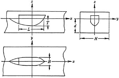
Figure 1: Definition of the Problem (a) Model in Towing Tank
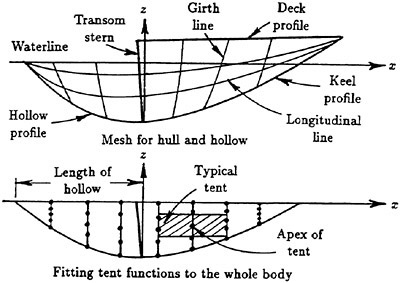
Figure 1: Definition of the Problem (b) Fitting Mesh to the Vessel
2.2 Modeling of the Hollow
The hollow behind the transom stern is modeled by assuming that it is a geometrically smooth addition to the vessel. Clearly, the water flow passes the transom-stern girth line in a well behaved manner and it is necessary to assume that the longitudinal derivatives of the mathematical body must be continuous there.
To this end, the vessel itself is first defined by means of an enclosing surface mesh, as described by Doctors (1993 and 1995c). In this scheme, the body is represented by a network of longitudinal and girth lines.
Specifically, the longitudinal lines are now extended rearward, beyond the transom. The assumption is made that all these longitudinal lines meet at the free surface at some focal point behind the vessel, whose coordinates are (xholl., 0, 0). The length of the hollow Lholl. is defined as the longitudinal distance between this point of confluence and the mean longitudinal coordinate of the immersed transom girth line.
We now focus our attention onto a single longitudinal line. In the first stage of the construction, we extend this line rearward utilizing its longitudinal x and radial r coordinates, in which
(1)
We now assume that the form of the line is a parabola, this being the simplest reasonable physical possibility. A simple analogy is to consider that the particles of water follow a trajectory in the radial plane which is similar to that of a jet of water acting under the influence of gravity. The relevant pair of parametric equations for the extension to the longitudinal line is
(2)
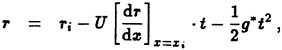
(3)
in which xi and ri are the coordinates of the relevant springing point of the hollow on the transom girth, U is the speed of the vessel (and hence the water past the stern, to the first order of approximation), and g* is the effective acceleration due to gravity, which is defined as
(4)
in which g is the acceleration due to gravity and fg is a, modifying constant. Finally, t is simply a parameter, which may be thought of as the physical time associated with the motion of a particle of water in this kinematic and dynamic model of the hollow. The x coordinate of the end of the hollow in this radial plane may now be calculated by substituting r=0 into Equation (2).
It must be made clear that this simple but robust model ignores certain obvious characteristics of the real hydrodynamic flow; principally this refers to the fact that the water on the surface of the hollow is not driven in this gravitational manner, but is affected by the full three-dimensional
fluid domain. It is anticipated that the factor fg can be used to correct for this defect.
Nevertheless, it is clear that this model possesses the following realistic and necessary attributes:
-
The transom-hollow transition is continuous in slope;
-
The curvature of the water surface is included;
-
The geometric aspects of the stern are considered realistically. These include the separate influence of transom-stern beam and draft, as well as the possibility of a non-zero rate of change of the sectional-area curve in the region of the stern of the hull;
-
The influence of sinkage and trim are included through their effect on the immersed geometry of the stern, and hence the shape of the hollow; and
-
The essential influence of speed, namely to increase the length of the hollow, is accounted for in a physically plausible manner.
The separate longitudinal lines will not generally meet at a single focus behind the vessel. This difficulty is overcome by computing a weighted focus, in which the weight is the element of transom girth associated with each longitudinal line. Furthermore, the possibility of an additional correction is permitted in this method by allowing the cavity to be stretched by the length factor fL.
The final stage in the construction of the hollow is to fit parabolas between the transom and the focus, ensuring continuity of slope, as already emphasized here. Also, a series of girth lines is fitted in order to fully define the hollow.
2.3 Wave Resistance of a Thin Ship in a Canal
For the present purpose, we will assume that the ferry is a monohull with a small beam-to-length ratio (the assumption of thin hulls) or a catamaran with thin hulls. This permits us to use the thin-ship or perturbation analysis of Michell (1898), Sretensky (1936) and Lunde (1951). The general formula for the wave resistance in a channel is
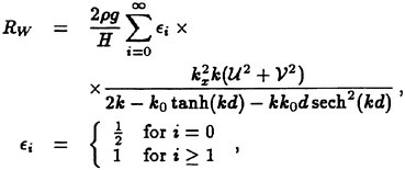
(5)
in which ρ is the water density.
The longitudinal and transverse wavenumbers in Equation (5) are
(6)
(7)
while the circular wavenumber k is given by the solution of the implicit dispersion relationship:
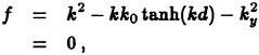
(8)
(9)
Finally, the fundamental wavenumber is
The index i of the summation in Equation (5) has been dropped from all the symbols except ∈, for the sake of brevity.
We next consider the two finite-depth wave functions in Equation (5), which were introduced by Doctors and Renilson (1992). They are:
(10)
(11)
in which the Michell deep-water wave functions P± and Q± are defined by
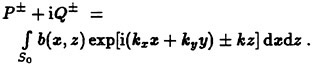
(12)
Here, b is the local beam of the hull (in the case of a monohull) or the demihull (in the case of a catamaran). The integration is to be performed over the centerplane area S0 of the hull (in the case of a monohull, for which y=0) or the two demihulls (in the case of a catamaran, for which y=±s/2 and s is the spacing between the centerplanes of the two demihulls).
2.4 Discretization of the Hull
It is necessary to discretize the hull for the purpose of the numerical evaluation of Equation (12). The simplest approach is to use rectangular panels, as indicated in Figure 1(b). The panels do not fit the centerplane exactly. However, it can be shown that the error associated with this non-fit at the edges is of the same order as the error incurred by assuming that the hull offset varies in a piecewise linear manner between the control points, as noted in the next paragraph.
Because of the linear nature of Equation (12) with respect to the hull beam, it is convenient to construct the hull from “tent functions”, which have base dimensions of 2Δx and 2Δz, and whose value is given by
(13)
in which f(x) increases linearly from zero at xj−Δx to unity at xj and then decreases linearly to zero at xj+Δx. Similarly, f(z) increases linearly from zero at zj−Δz to unity at zj and then decreases linearly to zero at zj+Δz.
The contribution to Equation (12) from the jth tent can be obtained by analytic integration, as shown by Doctors and Day (1995) and Day and Doctors (1997). The final result is:
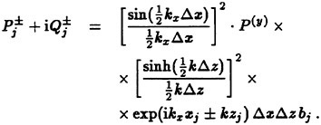
(14)
The upper row of tents (which are aligned along the waterline and for which zj is zero) only possess their lower halves and must therefore be expressed by a different formula:
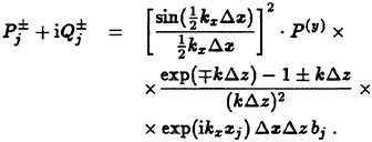
(15)
The influence of the demihull spacing in Equation (14) and Equation (15) is taken into account by means of the y-dependent factor:
(16)
The total resistance of the vessel is computed on the basis of the sum of the components of resistance, as follows:
(17)
Here, a wave-resistance form factor fW has been applied to the computed linearized wave resistance, an idea which is analogous to that behind the traditional (frictional-resistance) form factor. The similarity lies in that both factors are empirical corrections for analyses that are considered to be accurate in the limit of a very thin hull form.
The second term in Equation (17) is the hydrostatic resistance:
(18)
in which Ttran. is the draft at the transom; this is located at the longitudinal coordinate xtran.. The term results from the fact that the transom is considered to “run dry”.
The third term in Equation (17) is the frictional resistance RF, estimated using the 1957 International Towing Tank Committee (ITTC) formula, described by Lewis (1988, Section 3.5). The usual form factor fF has been applied here. The fourth term in Equation (17) is the correlation allowance RA, which is assumed to be zero for the hydraulically smooth test model.
The last term in Equation (17) is the aerodynamic resistance Raero., which can be approximated by the formula
(19)
where Aref. is the reference area of the vessel and CD is the drag coefficient, and the speed of the air flow relative to the craft can be expressed as
in which Uwind is the speed of the wind, with a positive value indicating a “tail” wind. The aerodynamic term has also been ignored in the current work.
Table 1: Geometric Functions
|
Index |
Function |
|
1 |
1 |
|
2 |
Β/L |
|
3 |
B/T |
|
4 |
CP |
|
5 |
CB(B/L)(L/s) |
|
6 |
(1)2 |
|
7 |
(B/L)2 |
|
8 |
(B/T)2 |
|
9 |
(CP)2 |
|
10 |
[CB(B/L)(L/s)]2 |
|
11 |
1 · F |
|
12 |
(B/L) · F |
|
13 |
(B/T) · F |
|
14 |
CP · F |
|
15 |
CB(B/L)(L/s) · F |
2.5 Numerical Convergence Tests
Some tests were done in order to gain an understanding of the number of panels typically needed to achieve converged results for the wave resistance. For a standard Wigley hull, it was found that a panel layout of 40×8 (in the longitudinal and vertical directions, respectively) results in an estimated discretization error of 0.1% in the wave resistance over the range of Froude numbers of interest. For similar reasons, the infinite series in Equation (5) was truncated at the point where the dimensionless transverse wave number kyL was around 500.
3 Application of Form Factors
3.1 Assumed Shape Functions
We consider that the two form factors in Equation (17) can be approximated in the following manner:
(20)
(21)
in which aW,i and aF,i are constants to be found and fi are functions of the hull geometry.
Table 2: The Wigley Models
|
Ship Model |
Length of Parallel Model Body LP (m) |
Beam Β (m) |
Draft T (m) |
Prismatic Coefficient CP |
|
1 |
0.000 |
0.30 |
0.18750 |
0.6666 |
|
2† |
0.000 |
0.15 |
0.09375 |
0.6666 |
|
3 |
0.000 |
0.30 |
0.09375 |
0.6666 |
|
4 |
0.000 |
0.30 |
0.04688 |
0.6666 |
|
5 |
0.600 |
0.15 |
0.09375 |
0.8000 |
|
6 |
0.375 |
0.15 |
0.09375 |
0.7500 |
|
7 |
0.825 |
0.15 |
0.09375 |
0.8500 |
|
8 |
1.050 |
0.15 |
0.09375 |
0.9000 |
|
9 |
1.275 |
0.15 |
0.09375 |
0.9500 |
|
10 |
0.150 |
0.15 |
0.09375 |
0.7000 |
|
† The parent hull |
||||
The particular choice of functions used in the present investigation is listed in Table 1.
Previous work reported by Doctors and Day (1997) and Doctors (1998) showed that even selecting just the first function (a constant) was sufficient to provide a greatly improved agreement between the predictions for the total resistance and the experimental data.
3.2 Solution for Optimal Factors
The method of least-squares was used to minimize the error in the fit of the functions given by Equations (20) and (21). The application of this procedure over the Μ experimental points leads to the following set of equations:

(22)
(23)
(24)
(25)
(26)
Table 3: The Twelve Lego Ship Models
|
Ship Model |
Length of Parallel Model Body LP (m) |
Length of Run LR (m) |
Length L (m) |
Prismatic Coefficient CP |
|
1 |
0.000 |
0.0000 |
0.7500 |
0.6666 |
|
2 |
0.000 |
0.1875 |
0.9375 |
0.7290 |
|
3 |
0.000 |
0.3750 |
1.1250 |
0.7499 |
|
4 |
0.000 |
0.5625 |
1.3125 |
0.7290 |
|
5 |
0.750 |
0.0000 |
1.5000 |
0.8332 |
|
6 |
0.750 |
0.1875 |
1.6875 |
0.8494 |
|
7 |
0.750 |
0.3750 |
1.8750 |
0.8499 |
|
8 |
0.750 |
0.5625 |
2.0625 |
0.8275 |
|
9 |
1.500 |
0.0000 |
2.2500 |
0.8888 |
|
10 |
1.500 |
0.1875 |
2.4375 |
0.8957 |
|
11 |
1.500 |
0.3750 |
2.6250 |
0.8928 |
|
12 |
1.500 |
0.5625 |
2.8125 |
0.8735 |
There are up to 2N coefficients to be determined, Ν coefficients for the wave-resistance factor and Ν coefficients for the fractional-resistance factor. The singly-primed summation in this equation indicates that preset terms are to be omitted. This can be accomplished by choosing values of aW,i and aF,i which are not to be included in the optimization process. Such terms (only) then have to be included in the doubly-primed summation.
4 Test Series
4.1 Modified Wigley-Hull Series
The first of the three hull types that was tested was a so-called modified Wigley hull. This form has parabolic sections and parabolic waterplanes, as first described by Wigley (1934). A total of ten models was constructed, all of length 1.5 m. Eight of these models were derived from the parent, or standard, hull by introducing a parallel middle-body section while keeping the overall length fixed. In this way, hulls with a different prismatic coefficent CP were created.
The remaining three models were created by altering the beam and draft from the parent
Table 4: The Ten SIHE Ship Models
|
Ship Model |
SIHE Designation |
Length-to-Beam Ratio L/B |
Beam-to-Draft Ratio L/T |
Slenderness Coefficient L/∇1/3 |
|
1 |
3b |
7.00 |
2.0 |
6.288 |
|
2 |
4a |
10.40 |
1.5 |
7.439 |
|
3 |
4b |
9.00 |
2.0 |
7.435 |
|
4 |
4c |
8.00 |
2.5 |
7.404 |
|
5 |
5a |
12.80 |
1.5 |
8.543 |
|
6 |
5b |
11.00 |
2.0 |
8.499 |
|
7 |
5c |
9.90 |
2.5 |
8.535 |
|
8 |
6a |
15.10 |
1.5 |
9.538 |
|
9 |
6b |
13.10 |
2.0 |
9.549 |
|
10 |
6c |
11.70 |
2.5 |
9.540 |
hull. The models were run in a towing tank with width Η of 3.5 m and a standard water depth d of 1.5 m. Furthermore, the parent hull was also run as a catamaran. These models are listed in Table 2.
4.2 Lego Ship-Model Series
The second series of hulls was developed with the intention of studying the hydrodynamics of transom sterns. Doctors (1998) provided the details of the hull segments from which the ship models were assembled. There was a total of seven segments. The bow and stern segments have parabolic waterplanes. The bow segments, stern segments, and the parallel middle-body segments all possess parabolic cross sections. Figure 2(a) shows pictorial views of one of the test models. Table 3 lists the details of these so-called Lego model series. Each model had a beam B of 0.150 m and a draft T of 0.09375 m. The bow section was 0.750 m in length.
4.3 Southampton Institute of Higher Education Series
The third series of ship models relates to the tests reported in particular by Molland, Wellicome, and Couser (1994a). There are currently ten models in the set. The models were each tested as a monohull as well as a catamaran with four different demihulls spacings, yielding 50 geometric configurations
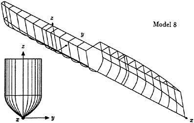
Figure 2: Sample Ship Models (a) Lego Ship-Model Series
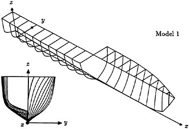
Figure 2: Sample Ship Models (b) SIHE Series
in total. These models are an outgrowth of the original National Physical Laboratory (NPL) tests described by Bailey (1976) and were derived by simple affine transformations of those original hulls. Further research of this nature was performed on these models and was reported by Insel and Molland (1991) and Molland, Wellicome, and Couser (1996).
Table 4 lists the principal features of these models, which all possessed a length L of 1.60 m, a block coefficient CB of 0.3941, a prismatic coefficient CP of 0.6878, and a maximum-section coefficient CM of 0.5731. The models were tested in the towing tank of the Southampton Institute of Higher Education (SIHE). This tank has a width of 3.7 m and a water depth of 1.85 m. The parent hull is depicted in Figure 2(b). (The numerical figures for the geometric data quoted here differ in some cases by up to 0.75% from those reported by Bailey. These discrepancies presumably relate to the vagaries of numerical techniques.)
5 Results
5.1 Unadapted Thin-Ship Theory
The major part of the analysis presented here relates to the SIHE series. We start by illustrating the effectiveness of the straightforward Michell theory together with the ITTC estimate of the frictional resistance, with form factors fW and fF of unity, indicated by Func.=0 in Figure 3 for Model 1 and Figure 4 for Model 9. These two models represent the extreme cases in terms of the slenderness coefficient L/∇1/3. Here, L is the vessel length and ∇ is its displaced volume. These graphs show a plot of the specific resistance R/W against the Froude number ![]() .
.
The agreement in all cases is qualitatively reasonable, except perhaps for the case of the closely-spaced demihulls, when s/L=0.2, where there is a pronounced interference hump. Presumably the lack of a transverse dipole distribution to impose the Kutta condition at the two sterns is the explanation for this result. It can also be observed that the pure theory generally provides an underprediction. However, an additional point is that there is an overprediction at the very low speeds, due to the fact that the theory has assumed that the stern runs “dry”. In actuality, the transom stern would be partly wetted and this would reduce the drag suffered by the vessel.
5.2 Use of Form Factors
We now examine the greatly improved accuracy that can be obtained by using appropriate form factors. The corresponding results from Figure 3 and Figure 4 are now re-calculated and presented in Figure 5 and Figure 6. The form-factor function Func. noted on the plots is a binary code made up of components, in which 20=1 indicates the use of
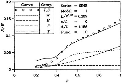
Figure 3: Resistance Components for SIHE Series Model 1 (a) s/L=0
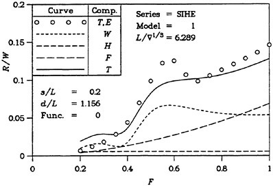
Figure 3: Resistance Components for SIHE Series Model 1 (b) s/L=0.2
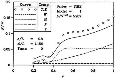
Figure 3: Resistance Components for SIHE Series Model 1 (c) s/L=0.3
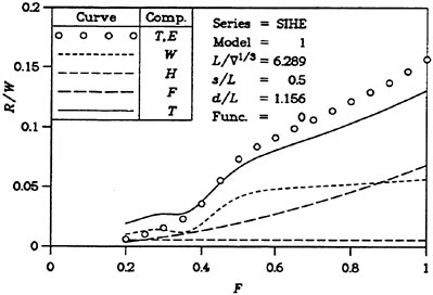
Figure 3: Resistance Components for SIHE Series Model 1 (d) s/L=0.5
the first term in Table 1, 21=2 indicates the use of the second term, and so on. The graphs show trials with various values of Func., including “0”, already noted. The value “1” implies the use of a constant factor, the value “3” indicates a linear function of Β/L, and the value “727” indicates that terms 1, 2, 3, 5, 7, 8, and 10 from Table 1 have been used.
The data shows that considerable improvement in the accuracy can be achieved in this manner. Near perfect agreement can be achieved in the last case, except for the awkward hump for the closely-spaced demihulls, already referred to above.
Finally, Table 5 shows a complete set of eight test cases. The first case with Func.=0
Table 5: Summary of Results
|
Function Code Func. |
Average Optimal Wave Form Factor fW |
Average Optimal Frictional Form Factor fF |
Root-Mean-Square Error in Total Specific Resistance eRMS |
|
0 |
1.000 |
1.000 |
2.470×10⁻² |
|
1 |
0.941 |
1.389 |
6.762×10⁻³ |
|
3 |
1.018 |
1.339 |
6.507×10⁻³ |
|
7 |
1.066 |
1.312 |
6.407×10⁻³ |
|
23 |
1.047 |
1.320 |
4.979×10⁻³ |
|
87 |
1.039 |
1.322 |
4.928×10⁻³ |
|
215 |
1.033 |
1.321 |
4.835×10⁻³ |
|
727 |
1.007 |
1.335 |
3.314×10⁻³ |
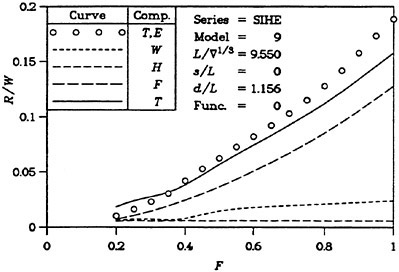
Figure 4: Resistance Components for SIHE Series Model 9 (a) s/L=0
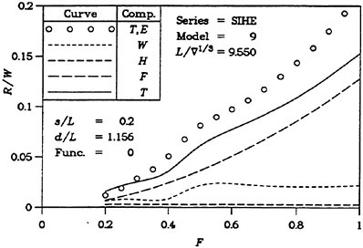
Figure 4: Resistance Components for SIHE Series Model 9 (b) s/L=0.2
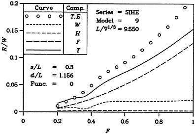
Figure 4: Resistance Components for SIHE Series Model 9 (c) s/L=0.3
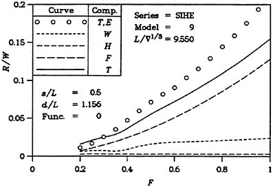
Figure 4: Resistance Components for SIHE Series Model 9 (d) s/L=0.5
is, of course, the unimproved theory. The ensuing seven cases show successive improvements in terms of the root-mean-square error in the values of R/W, showing a factor of reduction in the error of about 7.45. We also note that average optimal wave factors are typically around 1.0, while average optimal fractional factors range between 1.312 and 1.389.
5.3 Importance of Transom Hollow
The question of the transom-hollow factor-length fL in Equation (17) is now addressed in Figure 7 for Model 1 and in Figure 8 for Model 9. The monohull and one catamaran is considered in each case. It is interesting to observe that quite large variations in the choice of this factor can be used with little influence on the final results. The fact that the length of the hollow is relatively unimportant adds some justification to the use of a hollow that is even infinitely long. The infinite and simpler hollow has been employed by some researchers, including Day, Doctors, and Armstrong (1997).
5.4 Application to the Lego Ship-Model Series
As an additional test, the abovementioned formulation is now applied to four different models in the Lego series listed in Table 3. These are

Figure 5: Use of Form Factors for SIHE Series Model 1 (a) s/L=0
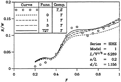
Figure 5: Use of Form Factors for SIHE Series Model 1 (b) s/L=0.2
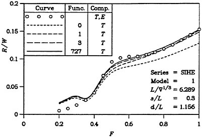
Figure 5: Use of Form Factors for SIHE Series Model 1 (c) s/L=0.3
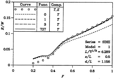
Figure 5: Use of Form Factors for SIHE Series Model 1 (d) s/L=0.5
shown in Figure 9. Although the actual values of the coefficients in Equations (20) and (21) have not been altered for this second series, one sees a similar improvement in accuracy described above. No doubt, even better agreement could be obtained by carrying out a regression analysis of a large range of vessel types—not just a single series, as was done in the present study.
5.5 Application to the Modified Wigley-Hull Series
The last test case relates to the modified Wigley hulls. Figure 10 shows the resistance components for the pure theory for two conditions, including a case of finite water depth. The jump in the theoretical resistance curve in Figure 10(a) should ideally be vertical; in this case, the horizontal distribution of the computed points coincided with that of the experimental points and hence the jump occurs over a finite change in the Froude number. Improved correlation between the (modified) theory and the experimental data is demonstrated in the two parts of Figure 11, even though the Wigley hulls were not used in the optimization process.
6 Concluding Remarks
The research presented here clearly demonstrates the considerable enhancement that can be obtained
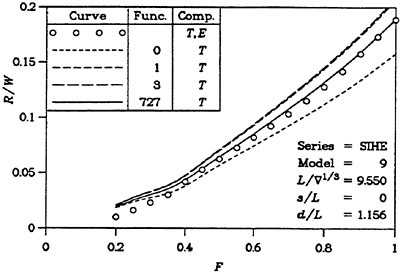
Figure 6: Use of Form Factors for SIHE Series Model 9 (a) s/L=0
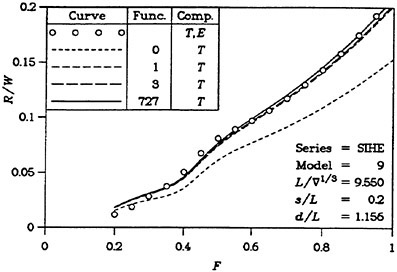
Figure 6: Use of Form Factors for SIHE Series Model 9 (b) s/L=0.2
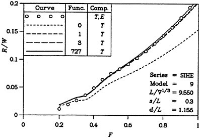
Figure 6: Use of Form Factors for SIHE Series Model 9 (c) s/L=0.3
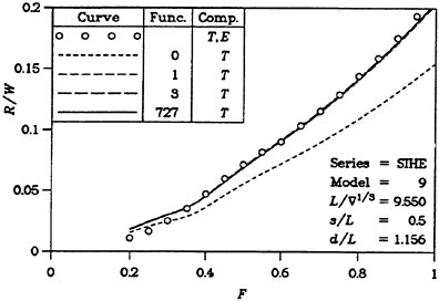
Figure 6: Use of Form Factors for SIHE Series Model 9 (d) s/L=0.5
by means of a simple type of correction to the traditional linearized theory. The number of constants required in the correction is relatively small in comparison to the number of constants required in a full, standard, regression of experimental data (in which no attempt is made to fit a wave-resistance theory). For example, in the work of Radojcic, Rodic, and Kostic (1997), in which the same hull series was analyzed, a total of 112 terms was required and, of course, the resulting formula would only apply to this one series of hulls.
A number of questions remains to be answered. These questions include the following:
-
What is the best choice of resistance function to analyze? Currently, the specific resistance R/W has been chosen. The more traditional resistance coefficient would be another choice and that would essentially weight the regression much more toward the lower speeds;
-
What is the best method of weighting the experimental points in the regression fit? At present, all points are considered to be of equal importance, even though there may be a number of experimental points bunched together in some regions of the resistance curve. Additional to this is the aspect that one could separately weight the Froude-number range of interest;
-
What is the best weighting between models? Currently, all models in the series were assumed to be of equal importance. It could be
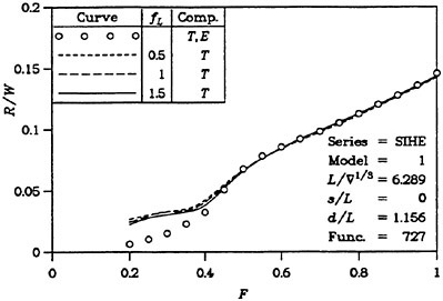
Figure 7: Effect of Transom-Hollow Factor for SIHE Series Model 1 (a) s/L=0
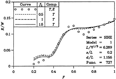
Figure 7: Effect of Transom-Hollow Factor for SIHE Series Model 1 (b) s/L=0.2
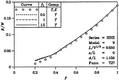
Figure 8: Effect of Transom-Hollow Factor for SIHE Series Model 9 (a) s/L=0

Figure 8: Effect of Transom-Hollow Factor for SIHE Series Model 9 (b) s/L=0.2
-
argued that one should add weighting to those hull types that are in more common use;
-
Should one use a staged regression? Currently all the hull models are fitted with the regression curves in a single process. The method allows one to fit, for example, the monohulls only (hence obtaining a high degree of accuracy in this case). Afterwards one can fit the catamarans, using only the geometric parameters relating to catamarans (spacing ratio s/L, essentially) and leaving the other parameters fixed. This approach would anchor the formulation on the monohulls as the more fundamental basis case of interest; and
-
Is it important to include a low-speed correction for the transom stern in order to model the partially-wetted case? It would seem possible that a simple theoretical model could be developed in order to correct the hydrostatic-resistance term RH in Equation (17).
7 Acknowledgments
The author is on partial secondment from The University of New South Wales to the Australian Maritime Engineering Cooperative Research Centre (AMECRC).
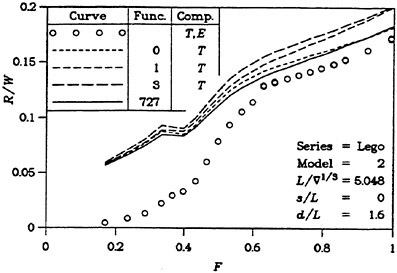
Figure 9: Use of Form Factors for Lego Series (a) Model 2
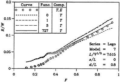
Figure 9: Use of Form Factors for Lego Series (b) Model 7
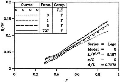
Figure 9: Use of Form Factors for Lego Series (c) Model 8
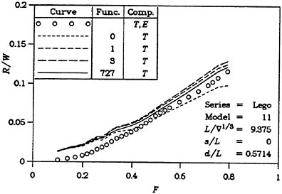
Figure 9: Use of Form Factors for Lego Series (d) Model 11
The author would also like to thank Mr G. Macfarlane and Mr B.McRae of the Australian Maritime College in Launceston, Tasmania, for their invaluable assistance with the conduct of the experiments in the towing tank.
He is most grateful to Dr P.Couser of AMECRC, at the Curtin University of Technology, in Perth, Western Australia, for his considerable support.
Finally, he would like to express his appreciation to Dr A.H.Day, of The University of Glasgow, in Glasgow, Scotland, for his active participation in the work that lead up to this project and for his continuing encouragement.
8 References
BAILEY, D.: “The NPL High Speed Round Bilge Displacement Hull Series”, Maritime Technology Monograph, Royal Institution of Naval Architects, No. 4, 90+ii pp (1976)
COUSER, P.R.: “An Investigation into the Performance of High-Speed Catamarans in Calm Water and Waves. Chapter 5: Theoretical Calculation of Calm Water Resistance”, University of Southampton, Department of Ship Science, Doctoral thesis, pp 91–122 (March 1996)
DAY, A.H. AND DOCTORS, L.J.: “Resistance Optimization of Displacement Vessels on the Basis of Principal Parameters”, J. Ship Research, Vol. 41, No. 4, pp 249–259 (December 1997)
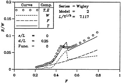
Figure 10: Resistance Components for Wigley Series (a) Model 2, s/L=0, d/L=0.25
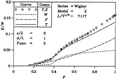
Figure 10: Resistance Components for Wigley Series (b) Model 2, s/L=0, d/L=1.0
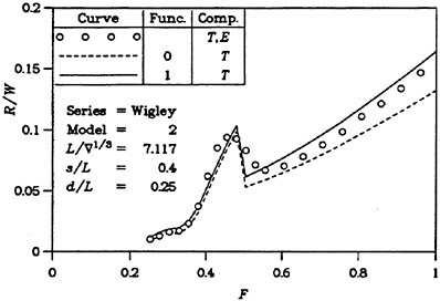
Figure 11: Use of Form Factors for Wigley Series (a) Model 2, a/L=0.4, d/L=0.25
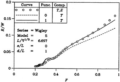
Figure 11: Use of Form Factors for Wigley Series (b) Model 5, s/L=0, d/L=1.0
DAY, A.H., DOCTORS, L.J., AND ARMSTRONG, N.A.: “Concept Evaluation for Large Very-High-Speed Vessels”, Proc. Fourth International Conference on Fast Sea Transportation (FAST ’97), Sydney, Australia, Vol. 1, pp 65–75 (July 1997)
DOCTORS, L.J.: “HYDROS: Integrated Software for the Analysis of the Hydrostatics and Hydrodynamics of Marine Vehicles”, Proc. Tenth International Maritime and Shipping Symposium (Ship-Shape 2000), University of New South Wales, Sydney, New South Wales, Vol. 1, pp 373–392 (November 1993)
DOCTORS, L.J.: “The Prediction of Ship Resistance by a Blended Theoretical and Experimental Method”, Proc. Seventh International Conference on Computational Methods and Experimental Measurements (CMEM ’95), Capri, Italy, pp 413–422 (May 1995)
DOCTORS, L.J.: “A Practical Method of Prediction of Ship Resistance for Displacement Vessels”, Proc. Sixth International Symposium on Practical Design of Ships and Mobile Units (PRADS ’95), Society of Naval Architects of Korea, Seoul, Korea, Vol. 1, pp 648–659 (September 1995)
DOCTORS, L.J.: “A Versatile Hull-Generator Program”, Proc. Twenty-First Century Shipping Symposium, University of New South Wales, Sydney, New South Wales, pp 140–158, Discussion: 158–159 (November 1995)
DOCTORS, L.J.: “Modifications to the Michell Integral for Improved Prediction of Ship Resistance”, Proc. Twenty-Seventh Israel Conference on Mechanical Engineering, Technion, Haifa, Israel, 5 pp (May 1998)
DOCTORS, L.J. AND DAY, A.H.: “Hydrodynamically Optimal Hull Forms for River Ferries”, Proc. International Symposium on High-Speed Vessels for Transport and Defence, Royal Institution of Naval Architects, London, England, pp 5–1–5–15 (November 1995)
DOCTORS, L.J. AND DAY, A.H.: “Resistance Prediction for Transom-Stern Vessels”, Proc. Fourth International Conference on Fast Sea Transportation (FAST ’97), Sydney, Australia, Vol. 2, pp 743–750 (July 1997)
DOCTORS, L.J. AND RENILSON, M.R.: “Corrections for Finite-Water-Depth Effects on Ship Resistance”, Proc. Eleventh Australasian Fluid Mechanics Conference (11 AFMC), University of Tasmania, Hobart, Tasmania, Vol. 1, pp 663–666 (December 1992)
DOCTORS, L.J. AND RENILSON, M.R.: “The Influence of Demihull Separation and River Banks on the Resistance of a Catamaran”, Proc. Second International Conference on Fast Sea Transportation (FAST ’93), Yokohama, Japan, Vol. 2, pp 1231–1244 (December 1993)
DOCTORS, L.J, RENILSON, M.R., PARKER, G., AND HORNSBY, N.: “Waves and Wave Resistance of a High-Speed River Catamaran”, Proc. First International Conference on Fast Sea Transportation (FAST ’91), Norwegian Institute of Technology, Trondheim, Norway, Vol. 1, pp 35–52 (June 1991)
INSEL, M. AND MOLLAND, A.F.: “An Investigation into the Resistance Components of High Speed Displacement Catamarans”, Trans. Royal Institution of Naval Architects, 11 pp, Discussion: 9 pp (April 1991)
LEWIS, E.V. (ED.): Principles of Naval Architecture: Volume II. Resistance, Propulsion and Vibration, Society of Naval Architects and Marine Engineers, Jersey City, New Jersey, 327+vi pp (1988)
LUNDE, J.K.: “On the Linearized Theory of Wave Resistance for Displacement Ships in Steady and Accelerated Motion”, Trans. Society of Naval Architects and Marine Engineers, Vol. 59, pp 25–76, Discussion: 76–85 (December 1951)
MICHELL, J.H.: “The Wave Resistance of a Ship”, Philosophical Magazine, London, Series 5, Vol. 45, pp 106–123 (1898)
MOLLAND, A.F., AND LEE, A.R.: “An Investigation into the Effect of Prismatic Coefficient on Catamaran Resistance”, Trans. Royal Institution of Naval Architects, 6 pp (1997)
MOLLAND, A.F., WELLICOME, J.F., AND COUSER, P.R.: “Resistance Experiments on a Systematic Series of High Speed Displacement Catamaran Forms: Variation of Length-Displacement Ratio and Breadth-Draught Ratio”, University of Southampton, Department of Ship Science, Report 71, 82+i pp (March 1994)
MOLLAND, A.F., WELLICOME, J.F., AND COUSER, P.R.: “Theoretical Prediction of the Wave Resistance of Slender Hull Forms in Catamaran Configurations”, University of Southampton, Department of Ship Science, Report 72, 24+i pp (March 1994)
MOLLAND, A.F., WELLICOME, J.F., AND COUSER, P.R.: “Resistance Experiments on a Systematic Series of High Speed Displacement Catamaran Forms: Variation of Length-Displacement Ratio and Breadth-Draught Ratio”, Trans. Royal Institution of Naval Architects, Vol. 138, pp 55–68, Discussion: 69–71 (1996)
RADOJCIC, D., RODIC, T., AND KOSTIC, N.: “Resistance and Trim Predictions for the NPL High Speed Round Bilge Displacement Hull Series”, Proc. International Symposium on Power, Performance and Operability of Small Craft, Royal Institution of Naval Architects, Southampton, England, pp 10.1–10.14 (September 1997)
SRETENSKY, L.N.: “On the Wave-Making Resistance of a Ship Moving along in a Canal”, Philosophical Magazine, Series 7, Supplement, Vol. 22, No. 150, pp 1005–1013 (November 1936)
TUCK, E.O.: “The Wave Resistance Formula of J.H.Michell (1898) and its Significance to Recent Research in Ship Hydrodynamics”, J. Australian Mathematical Society, Series B, Vol. 30, pp 365–377 (1989)
WIGLEY, W.C.S.: “A Comparison of Experiment and Calculated Wave-Profiles and Wave-Resistances for a Form Having Parabolic Waterlines”, Proc. Royal Society of London, Series A, Vol. 144, No. 851, pp 144–159+4 plates (March 1934)
DISCUSSION
C.Scragg
Science Applications International Corporation, USA
Prof. Doctors lists a number of parameters for regression. Although several of the parameters include Froude number, the final form factor seems to include only geometric parameters. This seems surprising in light of the fact that one of the more common deficiencies in the results of Michelľs integral is the exaggerated humps and hollows in CW versus Froude number. Please comment.
AUTHOR’S REPLY
Dr. Scragg has correctly noted that the particular functional variations of the form factors presented in this paper relate to geometric parameters alone, even though the possibility of dependence on Froude number was included in the computer program.
Some later work reported by Doctors (1998) in the additional reference showed that including Froude number-dependent terms does not indeed improve the accuracy in the sense that better correlation between theory and experiment can definitely be achieved. A further reduction in error in the specific resistance (of a factor of about two) to around 0.5% was reported there. (In that work, a more strenuous test of this approach was used because the ship resistance data was greatly expanded in terms of the range of beam-to-length ratio Β/L considered.)
Additional work in this area must therefore require a systematic study of a large range of functional variations in order to determine the best functions. No doubt, Froude number will continue to be important, as suggested by Dr. Scragg.
Doctors, L.J. “Modifications to the Mitchell Integral for Improved Prediction of Ship Resistance,” Proc. Twenty-Seventh Israel Conference on Mechanical Engineering, Technion, Haifa, Israel, 5 pp (May 1998)
DISCUSSION
G.Hearn
University of Newcastle Upon Tyne, United Kingdom
In optimization of the hull form, we know that “secondary parameters,” such as LES and LCF, are quite important in seakeeping. Likewise, LCB and B/T can be in conflict when seeking to cope with both seakeeping and resistance in hull form optimization. Knowing this, from theoretical studies [1,2], one might expect at least LCB to be a “function” in Table 1 of your paper. Is there any reason for its omission? Lack of experimental data regarding variation of LCB, say?
1. Hearn and Wright, FAST ’97, Australia
2. Hearn and Wright, OC ’98, Japan
AUTHOR’S REPLY
Professor Hearn is, of course, quite correct in suggesting that the longitudinal center of buoyancy LCB and the longitudinal center of flotation LCF should play an important role in determining the wave-resistance form factor and the frictional-resistance form factor.
The experimental data available to the author centered on the usual geometric ratios involving length, beam, draft, and demihull spacing (in the case of a catamaran). There is no doubt that with sufficient data, it would be advisable to utilize the additional “secondary parameters” noted by the discusser. In this way, improved accuracy would no doubt be achieved in the curve-fitting process.
Some Remarks on the Accuracy of Wave Resistance Determination from Wave Measurements Along a Parallel Cut
F.Lalli, F.Di Felice, P.Esposito, A.Moriconi (Istituto Nazionale per Studi ed Esperienze di Architettura Navale, Italy),
R.Piscopia (Universitá di Roma La Sapienza, Italy)
Abstract
In the present work some of the main error sources in the wave pattern resistance determination were investigated. The experimental data obtained at the Italian Ship Model Basin (longitudinal wave profiles generated by the steady motion of the Series 60 model and a hard chine Catamaran) were analyzed. It was found that, within the range of Froude numbers tested (.225≤Fr≤.345 for the Series 60 and .5≤Fr≤1 for the Catamaran) two sources of uncertainty play a significant role: (i) the presence of a wave pattern generated by the air pressure disturbance, related to the carriage motion, and (ii) the unsteadiness of the free surface flow (precision error). The propagation of the experimental errors in the wave resistance determination by the longitudinal cut method was next examined: the wave resistance coefficient shows a reasonable error band and the comparison with numerical results as well as with experimental data available in the literature shows a satisfactory agreement. Moreover, the errors related to the truncation of the wave profile, as well as to the transverse location of the probe, typical of the longitudinal cut method, were estimated. Systematic tests were performed by means of a numerical approach, which allows one to compare the wave resistance evaluated by the longitudinal cut method (applied in this case to the computed wave profiles) with the value obtained by pressure integration on the hull. As a result, in a sufficiently wide tank (b≥12 m) the longitudinal cut method can be applied without introducing any severe limitation for the model length, provided the wave profiles are measured at a proper transverse distance.
1. Introduction
The determination of the wave resistance of a ship model from measurement of the wave pattern received remarkable attention in the sixties and seventies (Newman, 1963; Sharma, 1966; Eggers et al., 1967; Wehausen, 1973). Though this component of the total resistance is usually (at least, at low Froude numbers) smaller than the viscous resistance, it is “…more amenable to treatment through the alteration and therefore important for the designer…” (Eggers et al, 1967). Moreover, as stated by Sharma (1966), “..it is an empirical fact that optimum design of least total resistance generally display the least surface disturbance in the vicinity of the bow”. Wehausen (1973) goes over the same subject again: “…experience and observation have shown that optimum design (from the standpoint of resistance) are those that make the smallest waves”.
Several methods were proposed (Eggers et al., 1967), to obtain the wave resistance by means of wave pattern analysis, all based on the linear potential flow model. The most popular techniques are those based on the analysis of wave profiles parallel to the model velocity: longitudinal cut method (LCM) (Newman, 1963; Sharma, 1966; Moran and Landweber, 1972) and matrix method (Hogben and Standing, 1974). These methods are generally preferred to the other ones since require only wave measurements at fixed points, and the wave profiles do intersect only partly the viscous wake region; on the other hand, infinitely long records of the wave height are needed in the application of LCM: suitable corrections for truncation errors were therefore proposed.
Several years later, wave pattern analysis was re-examined in the framework of potential flow numerical simulation, to obtain an algorithm for the evaluation of wave resistance more reliable than direct pressure integration on the hull (Nakos, 1991): in this case, transverse cut technique was preferred.
More recently, the problem of direct experimental determination of the wave resistance was revisited by Dumez and Cordier (1996), following the general trend in the framework of data quality control in towing tanks. In their paper the accuracy of wave pattern analysis was studied: the authors claim that severe limitations are needed for the ratio b/L (tanks width over model length) in the application of LCM, because of wave profiles truncation due to the reflection at the tank wall; more precisely, they state that
“…in order to obtain reasonably accurate (error<5%) wave pattern resistance estimates with LCM, for displacement vessels with significant wave making component (Fr<.4) the required b/L is about 5.”
In the present work a careful study was performed about some of the most important experimental error sources in the wave resistance determination by LCM: (i) errors due to the measurement chain, (ii) errors typical of the experimental facility (waves due to the carriage motion), (iii) errors related to the repeatability of the towing tests (flow unsteadiness, free surface perturbations in the tank, etc.).
Several towing tests were performed at the Italian Ship Basin with a conventional ship model (Series 60, .225≤Fr≤.345) as well as with a nonconventional one (Catamaran, .5≤Fr≤1). The wave profiles were measured by an array of capacitance wire probes. The uncertainty related to the experimental technique was analyzed by performing several calibration tests, whereas the error related to the air pressure disturbance induced by the carriage motion was studied by towing tests performed without any model. Moreover, in order to estimate the precision errors related to the towing tests, the experiments were repeated at least 7 times, for every Froude number tested. The results obtained show that the measurements performed by wire probes (capacitance or resistance ones) are sufficiently accurate, suitable for the application of LCM; on the other hand, the effects related to carriage waves and flow unsteadiness are significant sources of experimental uncertainty.
Next, the propagation of experimental errors in the wave resistance determination through LCM was examined, for both the Series 60 and the Catamaran. The 95% confidence interval related to the wave resistance coefficient shows a rather narrow error band and the comparison with the numerical wave resistance as well as with experimental data available in the literature shows a satisfactory agreement.
Furthermore, the errors typical of the mathematical model related to LCM were studied; in particular, the wave resistance coefficient dependence on transverse location of the wave profile and the effects of truncation were analyzed by numerical experiments: the wave pattern around a submerged prolate spheroid (conventional hull case) as well as around a couple of submerged prolate spheroids (twin hull case) was computed by a numerical code (Lalli, 1997) and the longitudinal profiles were analyzed by LCM. The obtained wave resistance was then compared with the value given by pressure integration on the body surface, in order to estimate the error due to truncation. The results of the present numerical analysis lead to much less pessimistic conclusions about the accuracy of LCM, with respect to the mentioned work by Dumez and Cordier: as a result, in sufficiently wide tank (b≥12m) this procedure can be applied without introducing any significant limitation for the model length.
2. Experimental set-up
Towing tests in calm water were performed at the INSEAN tank (430 m long, 13.5 m wide and 6.5 m deep) for a conventional ship model (Series 60 in fixed model condition, CB=.6, L=6.096 m, Fr=.225, .250, .275, .300, .316, .330 and .345) as well as for a non-conventional one (high speed hard chine Catamaran, L=5.124 m, free model condition, Fr=.5, .6, .7, .8, .9 and 1.). The experimental equipment (Agostini et al., 1997) consists of a zinc plated steel arm supporting 8 probes, mounted at a known distance from the longitudinal tank axis. The capacitance probes consist of a .25 mm diameter and 20 cm long silver copper wire with teflon insulation, stretched in a brass support by a little spring. The electronic circuit is located near the probe in order to keep the cable’s capacity negligible with respect to the low capacity measured (~100 pF). Dynamic tests show that the probe behaviour can be considered almost like a linear system: unitary transfer function modulus and reasonable phase distortion up to 4÷5 Hz. In order to avoid induced electronic noise during the long distance covered by the signals, tension is converted into frequency. These signals are converted into direct tension again, in the range ±5 V. The analog signals are then digitized with a sampling frequency of 50 Hz and stored. A rather careful description of wire probes, pointing out the differences between resistance and capacitance ones, was given by Gadd (1975): the dynamic behaviour of the former type should be less affected by meniscus variation, provided the separation of probe wires is large compared with the height of the meniscus itself. In the present work this difference was not detected; on the other hand, the typical disadvantage of capacitance probe, due to water absorption by the insulator with the related response variation, can be overcome by careful and frequent calibration and, of course, by avoiding probe immersion for too long times. To obtain the exact position of the wave profile with respect to the model, the start of the acquisition is given by a photoelectric cell, located at a known distance from the arm longitudinal axis.
3. Wave Measurements
In the present work the following aspects related to wave measurement errors were examined:
-
errors due to the measurement chain (probe non linearity and hysteresis, signal conditioning de-
-
vice errors, amplifier errors, A/D conversion error, etc.)
-
errors due to the experimental facility (waves generated by the motion of the carriage)
-
towing test precision errors (flow unsteadiness, wave perturbations in the tank, trigger jitter, probes arm vibrations, carriage velocity errors, random environment effects, etc.)
Since the budgeting of the different errors of the measurement system components (probes, signal conditioners, tension/frequency converters, anti-aliasing filters and A/D converter) is difficult to evaluate, the behaviour of the measurement chain was investigated by some calibration tests (11 points within the range −10÷+10 cm), repeated once a day. The average calibration curve, with the related 95% confidence interval, is shown in figure 1: the light data scattering obtained shows that the achievable bias limit for calibration errors (~.5 mm) is suitable for the measurements of typical gravity waves.
To evaluate the error due to the experimental facility 15 carriage runs (without towing any model) were performed, at U=1.74 and 2.67 m/s (minimum and maximum speed foreseen for the Series 60 tests). Wave height measurement, with 95% confidence interval, obtained by using the t distribution (Taylor, 1988), is shown in figure 2 for the maximum velocity tested: the very narrow confidence interval confirms the good behaviour of the measurement chain, detected in calibration tests.
In order to estimate the precision error in the Series 60 experiments, the towing tests were repeated 10 times, for every Froude number. As an example, 10 wave height measurements, related to 4 probes, are shown in figure 3 (Fr=.316). It can be seen that a very high repeatability is achieved, taking into account that in some regions flow unsteadiness can be expected: upstream region (spilling breakers) and wake region, in which vorticity structures give rise to a sort of short crested ripples. Moreover, in the plot related to y/L=.076, at .5<x/L<1, the wave cut is very close to the model (up to 3 cm). In fig. 4 is plotted the 95% confidence precision error band UP, given by:
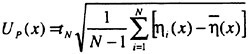
(1)
where ![]() is the ensemble average and tN is given by the t distribution. This figure shows very clearly that the precision error, mainly due to flow unsteadiness, and, in the second place, by free surface perturbations in the tank, plays a rather important role. Of course, far from the model the free surface flow appears to be more stable than in the near field.
is the ensemble average and tN is given by the t distribution. This figure shows very clearly that the precision error, mainly due to flow unsteadiness, and, in the second place, by free surface perturbations in the tank, plays a rather important role. Of course, far from the model the free surface flow appears to be more stable than in the near field.
Figure 5 shows 7 superimposed measurements of the waves generated by the carriage, at U=3.55 and 7.09 m/s (corresponding to Fr=.5 and 1. in the Catamaran towing tests), whereas in figure 6 the ensemble average values, at U=4.25, 5.67 and 7.09 m/s, are plotted in comparison. The wave pattern generated by the air pressure disturbance looks like a transverse wave system, with high frequencies perturbations; figure 7 shows that at the highest test speed these waves are characterized by an amplitude comparable with the waves generated by the model.
In figure 8 the 95% confidence interval is shown for 2 wave profiles measured at Fr=.5 (Catamaran towing tests); as it could be expected, in this case the precision error band is much larger: higher velocity as well as twin hull effects give rise to a more complicated wave pattern, characterized by remarkable unsteadiness. In particular, the spikes in the error bands are related to the interaction between the wave patterns generated by each hull.
On the whole, these data show that:
-
wave profile measurements are biased because of the presence of waves generated by the carriage motion: this effect grows, of course, as the speed increases; it is not easy to reduce this error;
-
the precision error, mainly related to flow unsteadiness, also becomes more significant as the speed increases: it seems appropriate to reduce this error by taking many readings and average them, in routine model tests; however, in the present work all the confidence intervals were computed by considering the precision index defined by (1), to show more clearly the effects of precision errors: in other words, in our results the confidence intervals are related only to one reading.
In order to estimate the effects of experimental errors in the evaluation of the wave resistance, only precision errors were taken into account, by elaborating all the measured profiles by LCM procedure. For all the Froude numbers tested, 10 longitudinal cuts for the Series 60 and 7 ones for the Catamaran, at every probe, were analysed. The results so obtained for the wave resistance were next elaborated statistically, at every Froude number, to obtain the confidence intervals. At the highest speeds (in practice, only for the Catamaran) the error related to the presence of the carriage disturbance will be taken into account in two ways, described in the next section.
4. Wave pattern analysis: the Longitudinal Cut Method
“…The existence of a far field in which linear theory is valid, breaking absent, and where the Kelvin wave pattern and the amplitude function have meaningful
existence has been pointed out, as well as a near field where various non-linear phenomena inevitably occur in the flow around a ship. It is the near field which must be predicted in order to know the wave resistance; the far field is its outer manifestation.” (Tulin, 1980). In the last decade many researchers dealt with nonlinear free surface problems, improving significantly the general understanding in this field. However, nobody proposed to take into account, in some sense, nonlinear effects in wave pattern analysis (at least, as far as the authors know): maybe the explanation of this can be found in the above quotation.
As known, in the steady 3-D problem, free waves (Havelock, 1934) can be represented in the elegant form
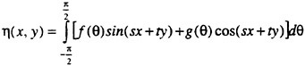
(2)
where s=k0secθ, t=k0sinθsec2θ, k0=g/U2, being θ the angle between the direction of propagation of the component wave and the model track; this expression can be obtained by solving Laplace equation, with linear boundary condition at the free surface, for instance with the method of separation of variables (Mandarino, 1983a) or, more simply, by means of a superposition of plane linear waves, characterized by phase velocity ![]() by taking into account the steadiness condition Vp=U·cosθ (Newman, 1978). The wave resistance can be then expressed in terms of the amplitude functions f(θ) and g(θ):
by taking into account the steadiness condition Vp=U·cosθ (Newman, 1978). The wave resistance can be then expressed in terms of the amplitude functions f(θ) and g(θ):
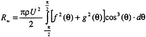
(3)
This formula shows very clearly how transverse waves give the main contribution to the wave resistance, but it is not used in practice; according to LCM (Newman, 1963; Sharma, 1966; Wehausen, 1973; Mandarino, 1983b), the wave resistance can be obtained from a parallel cut η(x,y0), taking into account the symmetry of the wave pattern:
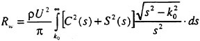
(4)
where
(5)
As known, the wave profile is required to extend to infinity downstream. In practice, the wave cut is truncated before reflection at the tank wall and the signal is prolonged by the asymptotic expression (s→k0) (Sharma, 1966):
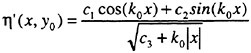
(6)
The coefficients c1, c2 and c3 are determined by fitting the measured wave height to the expression (6), using the tail of the truncated signal. In the paper by Eggers et al. (1967) is observed that, if the profile is sufficiently long, no serious error is introduced by assuming c3=0; our experience shows that this choice is suitable not only for sake of simplicity, but also because it leads to more accurate results. In fact, the profile given by (6), assuming c3≠0, strongly seems to depend on the length of the measured profile used in the least square fit procedure to obtain the coefficients c1, c2 and c3; on the contrary, when c3 is forced to be zero the behaviour is much more stable.
Generally, concerning with the transverse location of the probe, a limitation is given for the minimum distance from the hull (Dumez & Cordier, 1996). However, because of reflection at the tank wall, if the distance is too large the profile eventually becomes too short, and the resulting wave resistance can not be accurate. An optimum region will therefore exist, not too close to the model to avoid local effects and not too close to the tank wall. In our case, the measurements were performed by 8 probes, as described in a previous section, located at suitable distances from the tank axis; the wave resistance was then obtained by averaging the results of the elaboration in a proper region (more or less, .2<y/L<.5), in which the values seem to be stabilized. This problem is examined in next section.
As stated before, in order to investigate on the propagation of precision errors in the determination of wave resistance, we performed LCM elaboration (by means of a computer program developed at INSEAN (Agostini et al., 1997)) for all the measured wave profiles. Therefore, for every Froude number and at every transverse location 10 wave resistance values were obtained, next elaborated statistically. In figure 9a and 10a the wave resistance coefficient versus transverse direction y/L, with the 95% confidence interval/is plotted (Fr=.225 and .3) without truncation correction, whereas the latter is taken into ac-
count in figures 9b and 10b. In both cases a region in which the values of Cw can be considered constant can be detected; the ultimate value for Fr=.225 was then obtained by averaging the results concerned with the last 4 probes, and the 95% confidence interval UP is given by
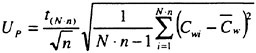
(7)
where n=4 and N=10. Likewise, for Fr=.3 the 4th, 5th, 6th and the 7th probe were taken into account.
In figures 11a,b the values of Cw (with and without the truncation correction respectively) are plotted as functions of the wave cut length: it is apparent that the behaviour, for both Froude numbers, is reasonably convergent, until the incoming of reflected wave: this stands clearly in figure 11b (Fr=.3). The truncation according to the Kelvin dihedral angle (xc in the figures) can be an effective tool. It is well known (Dumez and Cordier, 1996; Bruzzone et al., 1997) that at low Froude numbers the wave resistance is generated almost only by transverse waves. It could be therefore surprising that at Fr=.225 there is no significant difference between the corrected and the uncorrected value of Cw; maybe in this case the wave cut free from reflection contains a sufficient number of wavelengths, suitable to describe the spectrum accurately, and the truncation correction only makes the behaviour of Cw versus y/L lightly more regular. For Fr=.3, on the contrary, the contribution of truncation correction is more significant. The wave resistance of the Series 60 model was determined by following the described procedure for all the tested Froude numbers: the wave resistance coefficient, characterized by its error band, is compared in figure 12 with the numerical results obtained by the linear version of the computational code developed at INSEAN (Bassanini et al., 1994), as well as with experimental data available in literature (Kim and Jenkins, 1981). The agreement is rather satisfactory.
For the Catamaran, precision errors propagation was examined in the same way, whereas the effects related to the wave pattern generated by the carriage were studied in two ways:
-
by subtracting the carriage waves, for every probe and every Froude number, to the signals related to the corresponding model towing tests, and by computing the wave resistance in comparison with the wave resistance obtained from the original signals;
-
by computing the wave resistance related to the carriage waves in comparison with the wave resistance obtained from the signals concerned with the corresponding towing test.
As a result, though the presence of these waves affects significantly the accuracy of wave profiles measurements (~10% at U=7.09 m/s), their effects on wave resistance is less important (~1%).
In figures 13 and 14 are shown, respectively, Cw dependence on transverse distance y/L without and with the truncation correction, for Fr=.5 and .7; it is worth noticing that, at Fr=.5, the value of Cw related to y/L=.2 is characterized by a rather large error band, because of the presence of breaking and the consequent dispersion of the data (see figure 8). In both cases the 2nd, 3rd, 4th and the 5th probe were used in the evaluation of Cw. Figure 15 shows the dependence, for the 2nd wave cut (y/L=.272), on x/L. As in figure 11, xc indicates the truncation point related to Kelvin angle. At Fr=.5 (figure 15a) the convergence of Cw seems to be not reached, before reflection. As shown in the next section, this case is the most critical with respect to truncation errors; in fact, at Fr=.5÷.6 the transverse wave components still give a significant contribution, whereas the large wave length does not allow one to measure a sufficient number of periods before reflection. At Fr=.7 (figure 15b), on the contrary, since the contribution of transverse waves becomes negligible, the convergence is satisfactory and the difference between the corrected and uncorrected values is not significant. In figure 16 the corrected and, for Fr≥.7 also the uncorrected, wave resistance coefficients are plotted in comparison with the residual resistance coefficient.
Table 1: Series 60, y/L=.223
|
Froude |
Uη (mm) |
Uη (%) |
URw (kg) |
URw (%) |
|
.225 |
.7 |
4.8 |
.004 |
2.5 |
|
.250 |
.8 |
5.4 |
.006 |
2.5 |
|
.275 |
.8 |
2.8 |
.022 |
1,9 |
|
.300 |
.9 |
2.4 |
.034 |
1.4 |
|
.316 |
.9 |
2.1 |
.046 |
1.5 |
|
.330 |
1.2 |
2.3 |
.070 |
2.1 |
|
.345 |
1.5 |
2.6 |
.053 |
1.4 |
Table 2: Catamaran, y/L=.481
|
Froude |
Uη (mm) |
Uη (%) |
URw (kg) |
URw (%) |
|
.5 |
3.9 |
5.8 |
.233 |
2.1 |
|
.6 |
3.8 |
5.6 |
.216 |
2. |
|
.7 |
3.9 |
6.1 |
.143 |
1.7 |
|
.8 |
3.7 |
6.2 |
.278 |
3.8 |
|
.9 |
3.8 |
6.7 |
.097 |
1.2 |
|
1. |
4.1 |
6.5 |
.193 |
3. |
In table 1, 2 the errors bands, as functions of Froude number, are reported; the errors concerned with wave profiles are normalized with respect to the
maximum wave amplitude. LCM appears to be a well-conditioned procedure, since the normalized error on the wave resistance is always lower than the corresponding error on the wave profile.
5. Accuracy of the Longitudinal Cut Method
Some considerations about the accuracy of LCM were reported by Dumez and Cordier (1996). They suggested a limit for the transverse probe position (k0y≥ 5) and, for the truncation error ê, performed a statistical analysis (.3≤Fr≤1.): reasonably accurate (ê<5%) wave resistance can be obtained, provided the limitaton b/L>5 is fulfilled.
In the present work the behaviour of LCM was studied by means of a numerical code implementing linear boundary conditions at the free surface. The steady wave pattern around a submerged prolate spheroid was computed by a desingularized boundary integral method (Lalli, 1997) and the wave resistance, evaluated by LCM, is compared, for .3≤Fr ≤.8, with the value obtained by pressure integration. The submerged body example was preferred because in this case the pressure integral gives a very accurate value for the wave resistance. The results of the present analysis can be assumed sufficiently general in the hypothesis that the behaviour of the truncation error ê mostly depends on the Froude number, the ratio b/L and the ratio y/L. In fact, though two different shaped models generate two unlike free wave spectra, i.e. with a different distribution of energy between transverse and divergent systems, the problems related to the truncation of the wave profile probably depend mainly on the fundamental wave length. Dumez and Cordier (1996) came to the same conclusion on the basis of their experimental observations. Therefore, we assume ê=ê(y/L, b/L, Fr).
Systematic tests with the numerical code allow to obtain the function ê for several Froude numbers (see figures 17a÷17f). The dependency on b/L is taken into account by truncating the longitudinal profiles according to a perfect reflection law and to Kelvin angle. The calculation is performed in a rather large computational domain: a region extended 2L upstream, 13L downstream and 3.7L laterally is discretized by 39×162 desingularized elements; the submerged body is approximated by 40×16 flat panels.
The figures show that, for all the Froude numbers, in the vicinity of the body the elaboration of numerical wave profiles gives overestimated values for the wave resistance, because of the presence of local wave elevation effects. On the other hand, when the longitudinal profile is located too far from the model (y/b=.2÷.4) the wave resistance, as a function of y/L, shows a sharp peak. This is an effect of the truncation: in fact, if the wave profile is not long enough to include a significant part of transverse wave region, the correction given by (6) introduces a large error. Indeed, in such case the reconstruction of a transverse wave profile by extrapolating a signal related only to the divergent wave system is attempted. Though, in principle, the free surface along any longitudinal cut behaves asymptotically like (6), for finite values of x the ratio y/x shall be small, as observed by Gadd (1975). Therefore, an upper limit for the parameter y/b can be achieved: though this value seems to depend on Froude number, numerical solutions and experimental data seem to suggest y/b≤.2. Anyway, in all the figures, for all the Froude numbers tested, the presence of a region of reasonable accuracy is evident. This region, more or less, migrates far from the model as the Froude number grows up to .5÷.6, provide the ratio b/L is not too small; for Fr≥.7 the accuracy generally improves, since the contribution of transverse waves to the total wave resistance becomes less important, and the profile is no more required to be very long. In particular, for Fr=.8 the wave resistance evaluated without the truncation correction is more accurate with respect to the corrected value: in this case the main contribution to the wave resistance is given by divergent waves.
On the whole, the results shown (figures 17a ÷17f) point out the reasonably accurate behaviour of the method, with respect to the truncation error: in the worst case (Fr=.5÷.6, b/L=2) the error is about 6%. It is worth noticing that, if the tank is sufficiently wide (b≥12 m), the condition b/L≥2 is not a significant restriction for hull models length.
Finally, some more careful numerical investigations were performed for the twin hull case; the wave field past a couple of submerged spheroids, with the same mean geometrical characteristics of the Catamaran model, was computed (Yb/L=.0921, being Yb the model width, Hb/L=.224, being Hb the distance between the hulls). The computations were performed at Fr=.5, .6, .7 and .8 (figures 18a÷18d) with 40×32 flat panels on the body; grid dependence tests at the free surface (3366, 4880, 6532 and 8639 panels) show a rather satisfactory convergent behaviour. The extension of the computational domain was chosen according to the ratio b/L=2.635, the same of the experiments concerned with the Catamaran model.
Also in the twin hull example, it is confirmed that: (i) in the worst cases (Fr=.5÷.6) the error is
about 6% and (ii) at Fr≥..7 the wave resistance coefficient can be, more conveniently, computed without truncation correction.
6. Summary
The analysis carried out in the present work, concerned with the accuracy of experimental determination of the wave resistance, shows that:
-
wave profiles can be measured by (capacitance or resistance) wire probes with a sufficient accuracy, suitable for the longitudinal cut method, though the instrument is intrusive; moreover:
-
wave profile measurements are biased for the presence of waves generated by the carriage: this effect increases, of course, with the velocity;
-
precision error, mainly related to flow unsteadiness, also becomes more significant as the velocity increases: from a statistical point of view, it seems appropriate to reduce this error by taking many readings and average them, in routine model tests;
-
the propagation of experimental errors in the longitudinal cut method procedure shows that the wave resistance coefficient can be obtained with a reasonable confidence;
-
-
the main error, in the evaluation of wave resistance, is related to wave pattern analysis: it is well known that the longitudinal cut method is sensitive to wave profile truncation; the present analysis, based on numerical experiments, shows that:
-
generally, only a lower limit is given for the transverse location of the probe: this condition can be misleading; in fact, though along any parallel cut η(x, y0) → O(x−1/2), according to (6), in order to implement correctly the truncation correction at finite values of x, the ratio y/x shall be small (Gadd, 1975); as an example, experimental data (figure 14b) as well as numerical results (figure 18c), point out that the curve Cw (corrected) versus y/L shows a bump, related to the failure of the truncation correction (6)
 an upper limit for the transverse location of the probe should be therefore adopted, maybe in terms of the parameter y/b;
 -
errors related to wave profiles truncation, provided the transverse distance y/L is correctly chosen, are ≤6%; for Fr≥.7 it seems suitable to determine wave resistance without truncation correction.
-
Acknowledgements
The authors whish to acknowledge the contribution given by Carlo Agostini and Emanuele Millina in the design and set up of the experimental apparatus. This work was supported by Italian Ministero dei Trasporti e della Navigazione in the frame of INSEAN research plan 1994–96.
References
1. Agostini, C., Di Felice, F., Lalli, F., Millina, E., Moriconi, A. (1997). “Il metodo del taglio d’onda longitudinale per la determinazione sperimentale della resistenza d’onda”, Rapporto Tecnico INSEAN.
2. Bassanini, P., Bulgarelli, U., Campana, E., Lalli, F. (1994). “The Wave Resistance Problem in a Boundary Integral Formulation,” Surv. Math. Ind., Vol. 4.
3. Bruzzone, D., Cassella, P., Pensa, C., Scamardella, A., Zotti, I. (1997), “On the Hydrodynamic Characteristics of a High-Speed Catamaran with Round-Bilge Hull: Wave Resistance and Wave Pattern Experimental Tests and Numerical Calculations”, 4th International Conference on Fast Sea Transportation, Sydney, Australia.
4. Dumez, F.X., and Cordier, S. (1996). “Accuracy of Wave Pattern Analysis Methods in Towing Tanks,” 21st Symposium on Naval Hydrodynamics. Throndeim.
5. Eggers, K.W.H., Sharma, S.D., and Ward, L.W. (1967). “An Assessment of Some Experimental Methods for Determining the Wavemaking Characteristics of a Ship Form,” Transactions SNAME, vol. 75.
6. Gadd, G.E., (1975). “Wave Pattern Measurement”, 14th ITTC Report of the Resistance Committee.
7. Havelock, T.H. (1934). “The Calculation of Wave Resistance”, Proceedings of the Royal Society, vol. 144, Series A, 514–521.
8. Hogben, N., Standing, R.G. (1974). “Wave Pattern Resistance from Routine Model Tests”, Trans. Of the Royal Inst. Of Naval Architects.
9. Kim, Y.H., and Jenkins, D (1981). “Trim and Sinkage Effects on Wave Resistance with Series-60, CB=0.6,” DTNSRDC/SPD—1013–01.
10. Lalli, F. (1997). “On the Accuracy of Desingularized Boundary Integral Method in Free Surface Flow Problems,” International Journal for Numerical Methods in Fluids, vol. 25, 1163–1184.
11. Mandarino, M. (1983a). “Sul Problema delle Onde Libere in un Canale di Dimensioni Finite o Infinite,” Studi Marittimi.
12. Mandarino, M. (1983b). “Alcune Considerazioni sulla Determinazione Sperimentale della Resistenza d’Onda,” Studi Marittimi.
13. Moran, D.D., Landweber, L. (1972). “A Longitudinal-Cut Method for Determining Wavemaking Resistance”, Journal of Ship Research.
14. Nakos, D.E. (1991). “Transverse Wave Cut Analysis by a Rankine Panel Method,” 6th International Workshop on Water Waves and Floating Bodies.
15. Newman, J.N. (1963). “The Determination of Wave Resistance from Wave Measurements along a Parallel Cut,” Int. Seminar on Theoretical Wave Resistance, Univ. of Michigan.
16. Newman, J.N. (1978). Marine Hydrodynamics, MIT Press, Cambridge, MA.
17. Sharma, S.D. (1966). “An Attempted Application of Wave Analysis Techniques to Achieve Bow-Wave Reduction”, 6th Symposium of Naval Hydrodynamics, Washington D.C.
18. Taylor, J.L. (1988). Fundamentals of Measurement Error, Neff Instrument corporation.
19. Tulin, M.P. (1980). “Wave Resistance”, Report of the Resistance and Flow Committee, 19th ATTC, Ann Arbor..
20. Wehausen, J.V. (1973). “The Wave Resistance of Ships,” Advances in Applied Mechanics.
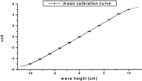
Figure 1: Typical probe calibration curve, with the related confidence interval
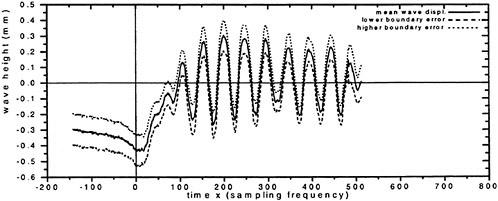
Figure 2: Wave height due to the carriage motion (moving pressure disturbance) with confidence interval at U 2.67 m/s
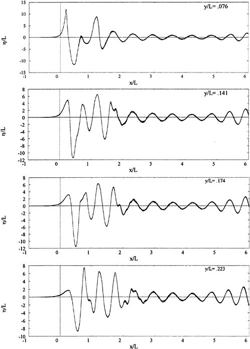
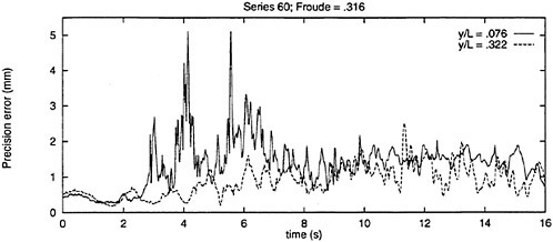
Figure 4: Precision error (95% confidence) along parallel cuts (Series 60, Froude=.316)
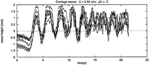
Figure 5a: Plot of 7 wave height measurement (wave pattern generated by the motion of the carriage, U=3.55 m/s)
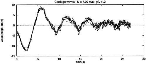
Figure 5b: As in figure 5a, at U=7.09 m/s
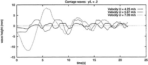
Figure 6: Average values of the waves height generated by the motion of the carriage
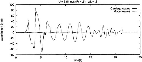
Figure 7a: Comparison between the average waves generated by the towed model (catamaran, Froude=.5) and the average waves generated only by the carriage at the same velocity (U=3.55 m/s), at y/L=.2
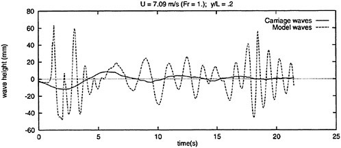
Figure 7b: As in figure 7a (Froude=1., U=7.09 m/s)
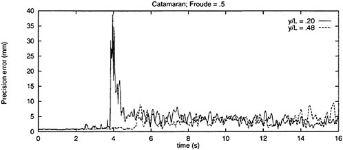
Figure 8: Precision error (95% confidence) along parallel cuts (Catamaran, Froude=.5)

Figure 9: Cw as a function of y/L (Series 60, Froude=.225); (a): without truncation correction, (b): with truncation correction)
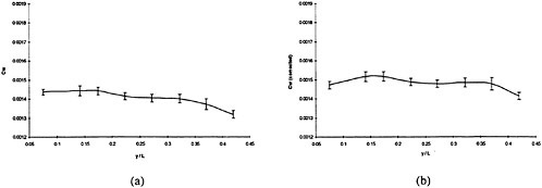
Figure 10: As in figure 9, at Froude=.3
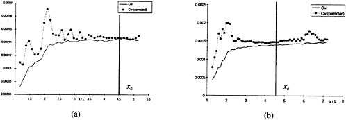
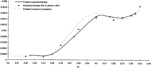
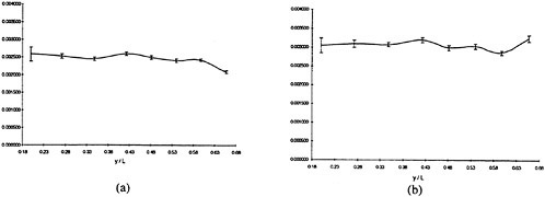
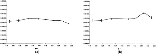
Figure 14: As in figure 13, at Froude=.7.
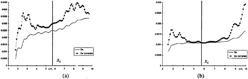
Figure 15: Cw versus x/L (Catamaran, y/L=.272); (a): Froude=.5, (b): Froude=.7
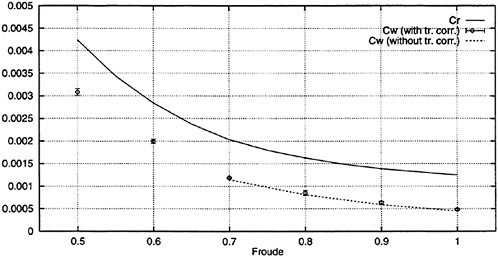
Figure 16: Cw versus Froude (Catamaran)
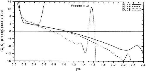
Figure 17a: Numerical computation of the potential flow past a submerged prolate spheroid: wave resistance coefficient error versus lateral position of the wave profile
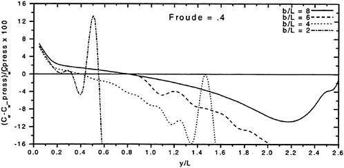
Figure 17b (as in figure 17a).
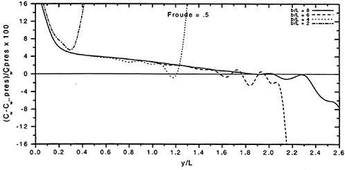
Figure 17c (as in figure 17a).
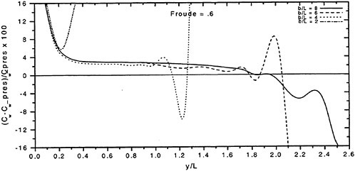
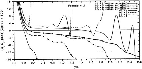
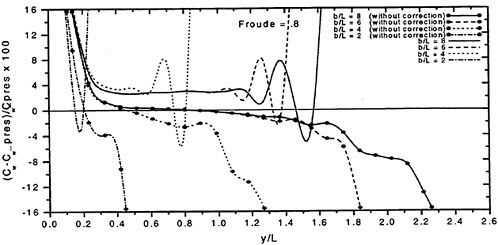
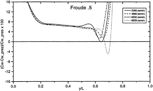
Figure 18a: Numerical computation of the potential flow past a couple of submerged prolate spheroids: wave resistance coefficient error versus lateral position of the wave profile (b/L=2.635)
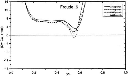
Figure 18b: As in figure 18a
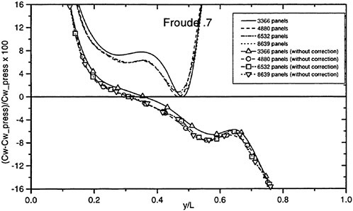

DISCUSSION
I.Zotti
University of Trieste, Italy
The authors are to be congratulated for having examined and presented the conclusions of a very specific and detailed analysis on the error sources in the wave pattern resistance determination. Nowadays, so many tools are available for the hydrodynamic analysis in ship design, both of numerical and experimental nature. Therefore, in the engineering community a great interest was born about the reliability, accuracy, and robustness of these techniques. In this work a very deep analysis on the main error sources related to wave pattern analysis is carried out, in particular for the longitudinal cut method. Uncertainty analysis shows that the propagation of the experimental errors in the determination of the wave resistance from a longitudinal cut does not affect significantly the result, also because the precision error decays rapidly in the far field: this is another reason to prefer the method of Sharma with the wave truncation with respect to the transverse cut method, based on wave measurements in a region including the wake, where viscous effects, and therefore flow unsteadiness, are very meaningful, and a more significant spreading of the results can be expected, with respect to figure 13 (at y/L=.2).
Generally, experimental data are used in order to validate numerical codes; in this paper numerical techniques are used in order to estimate the accuracy of an experimental technique. This methodology was also used by Moran and Landweber (1972) (ref. 13), and it seems to be the most suitable to examine the truncation error. Of course, this paper states that the main error is related to the truncation of the wave profile as well as to an inappropriate transverse distance of the wave profile from the model; however, the numerical analysis performed shows that such errors can be reduced to a reasonable value, by a proper implementation of the method.
It seems surprising that, sometimes, very important requirements for the correct applications of a procedure are forgotten, as time goes by. In fact, as stated in this paper, the indications related to the small value of the ratio y/x, for the validity of the asymptotic expression of the free surface at finite values of x, is not mentioned in recent work (ITTC’84; Dumez and Cordier, etc.). However, a little but dutiful remark can be made: a suggestion that the authors mention that also in the paper by Newman (1963) (ref. 15) this requirement was pointed out.
Finally, the mentioned problems concerned with the evaluation of the truncation correction coefficients (c1, c2, c3) could be more specified with a figure, since the least square fit procedure, if not carefully applied, can give rise to serious inaccuracies, as stated in this paper.
AUTHORS’ REPLY
The authors wish to thank Prof. Zotti for his kind and stimulating comments. Of course, Prof. Newman (ref. 15) pointed out the importance of the requirement y/x→0, in order to correctly implement the truncation correction. Unfortunately, the authors forgot to mention this in the present paper: in ref. 15 this remark appears as a footnote, and could pass unnoticed.
In figure 1, the accuracy of wave resistance, as a function of y/L, is shown. It is apparent that the truncation correction is rather unstable, in that wave resistance strongly depends on the length of the wave profile tail used in the least square fit procedure for the coefficients evaluation. Fortunately, when c3=0 the behavior becomes much more stable.
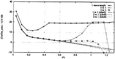
Figure 1. Numerical simulation of the wave pattern past a submerged prolate spheroid (Fr=.3): normalized error of the wave pattern resistance (with respect to the value given by pressure integration) as a function of y/L, varying the length of the computed profile tail (used for the evaluation of truncation correction coefficients).
Wave Resistance and Wave Patterns for High-Speed Crafts; Validation of Numerical Results by Model Test
S.Brizzolara, D.Bruzzone (University of Genoa, Italy),
P.Cassella (University of Naples, Italy),
A.Scamardella, I.Zotti (University of Trieste, Italy)
ABSTRACT
Some results from a cooperative research program on high-speed displacement crafts conducted by Genoa, Naples and Trieste Universities are described in this paper. Numerical wave resistance and wave pattern calculations by a boundary element method are compared with experimental results deriving from tests carried out in two towing tanks at different scales on some models of high speed marine vehicles. The presented cases are two catamarans and a monohull examined in the Froude number range up to 1.1. The numerical wave resistance has been obtained by both the pressure integration and the wave pattern analysis on a transverse cut downstream the ship. An extension of the numerical method based on a modified Newton iterative procedure to determine the running trim and sinkage is presented, discussed and compared with some of the experimental data. Towing tanks tests were carried out with the goal to obtain validation of the numerical results and indications on the resistance components, on the scale effects and on the interference phenomena between the demihulls of catamarans. In this perspective, total resistance, running trim, sinkage and wave pattern analysis based on the longitudinal cut procedure have been examined.
1. INTRODUCTION
Nowadays, from the comparison among the different operating high-speed crafts, it appears that the monohull and the catamaran arc the most diffused and can adequately satisfy the increasing demand for speed up in marine transportation.
A large number of theoretical and experimental investigations have been carried out so far on the hydrodynamics of these type of ships, but still some topics require further research. This is the case, for instance, of the prediction of their steady free surface flow and related forces by numerical calculations as well as the experimental procedures for the direct evaluation of their wave resistance from wave pattern analysis. These aspects are investigated in the present paper in which the joint application of a boundary element method [1], experimental wave pattern analysis and routine model tests are considered for some different hull forms typically employed for of high speed crafts.
From the visual observation of the characteristic flow of the tested models, a significant presence of spray was not observed during all the resistance model tests, so it was assumed to consider the hydrodynamic characteristics of high speed crafts in the examined Froude range in the same way as those of the traditional ships. Therefore, in order to have information on the ship resistance components and on the scale effects it was accepted that also for high speed crafts, as well as for traditional ships, the hydrodynamic total resistance can be split into the viscous and wavemaking components only.
The model tests have been carried out in two different towing tanks, where wave patterns and routine model data have been measured. The wave pattern analysis has been carried out by the longitudinal cut method with truncation corrections and by the multiple longitudinal cut method with reflections.
Similar tests and calculations were already carried, for purpose of validation, on more conventional hull forms, such as geosims of series 60, in the Froude number range Fn=0.2÷0.4 [2–3].
As far as the numerical method is concerned it must be remarked that for high speed hulls, though, in principle, the higher Froude numbers allow lower numbers of panels for the free surface representation, the prediction of the flow field is complicated by the importance of the running trim and sinkage which cannot be neglected and have a remarkable effect on the ship generated waves [4]. The existence of a transom stern further complicates the problem. Some applications already carried out on round-bilge monohulls and catamarans, where the experimental trim and sinkage values were considered in the calculations, emphasized these circumstances and, in addition, shown reasonable agreement between calculated and measured free wave spectra [5].
The comparison between the experimental and numerical results is carried out in terms of wave resistance, wave patterns and free wave spectra. The obtained results are promising, but, till now, because of the lack of sea trial data we are not able to evaluate their effective validity.
2. TESTED HULL FORMS AND MODELS
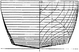
Figure 1—Monohull
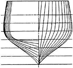
Figure 2—CAT.1
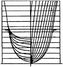
Figure 3—CAT.2
Table 1—Characteristics of the tested models
|
|
Monohull |
CAT.1 |
CAT.2A |
CAT.2B |
||||
|
|
A |
B |
Catam. |
Demihull |
Catam. |
Demihull |
Catam. |
Demihull |
|
Fn |
0.4–1.10 |
0.4–0.70 |
0.5–1.10 |
0.4–1.10 |
0.4–0.7 |
|||
|
L [m] |
3.900 |
1.545 |
3.030 |
2.500 |
1.250 |
|||
|
B [m] |
0.632 |
0.316 |
0.632 |
0.245 |
0.660 |
0.200 |
0.330 |
0.100 |
|
T [m] |
0.096 |
0.048 |
0.096 |
0.177 |
0.088 |
|||
|
V [m3] |
0.0768 |
0.0096 |
0.0608 |
0.0304 |
0.081 |
0.0405 |
0.102 |
0.00506 |
|
s/L |
– |
– |
0.225 |
– |
0.225 |
– |
0.225 |
– |
|
CB |
0.41 |
0.35 |
0.35 |
0.35 |
||||
|
L/V^1/3 |
9.175 |
7.706 |
9.708 |
5.778 |
7.280 |
2.675 |
7.281 |
|
|
L/B |
6.171 |
4.79 |
12.37 |
3.79 |
12.50 |
3.79 |
12.50 |
|
|
B/T |
6.583 |
6.58 |
2.55 |
3.73 |
1.13 |
3.75 |
1.14 |
|
The cooperative experimental investigation was carried out on models of three high speed crafts in the towing tank of the University of Naples (146 m×9.0 m ×4.2 m, maximum carriage speed 6 m/s) and in the towing tank of University of Trieste (50 m×3.1 m×1.6 m, maximum carriage speed 2.5 m/sec).
The chosen hull forms derive from one hard chine monohull operating in the Gulf of Naples (fig. 1) and from two round bilge symmetric catamarans. The demihull forms of the first catamaran, here named CAT1, are taken from series 64 (fig. 2), those of the second catamaran, here named CAT2, from an experimental research carried out at the University of Trieste (fig. 3),.
The size of the models were chosen taking into account the minimum acceptable dimensions of the models and the size and the maximum carriage speed of the two towing tanks. The model of CAT1 was built in wood and the off-sets of the demihull were checked using a model shaping machine. All the other models were constructed in GRP.
The main dimensions and the investigated range on Froude numbers are given in Table 1. The small models of the monohull and of CAT2 were tested in the towing tank of Trieste, all the other models were tested at the towing tank of Naples.
A complete set of measurements including total hydrodynamic resistance, running trim, sinkage and wave pattern analysis was performed for all the models. Capacity probes, which gave a good linear signal response with the wave height, were used for the measurement of the wave profiles.
The models were tested with towing point placed on the main bridge at the longitudinal center of gravity position and with a horizontal towing line direction. Turbulence stimulators were not used, since in the high Froude range a turbulence stimulator attached at the bow is not advisable because of the bow-up condition or of the spray. Total resistance, running trim and sinkage were measured together with wave pattern analysis.
The total resistance and its components were reduced to coefficients by means of the usual relation C=R/0.5ρSV2. By using the classical Froude procedure methodology of resistance components subdivision and using specifically the ITTC’57 model-ship correlation, we obtained the residual resistance coefficient CR=CT−CFo, being CFo the frictional resistance coefficient according to ITTC’57 frictional line.
The measured data were also analysed by ITTC’78 correlation methodology. For this purpose additional resistance tests were carried out at low speed by running the models with the transom emerged and with turbulence stimulators suitable to the model scale so to be able to calculate the form factor. The results and discussion are herein omitted since some of them are reported in previous papers.
Wave interference phenomena on the catamarans was also investigated by placing a probe between the demihulls in order to compare the inner wave profile with those ones measured outside both for the catamaran and for its isolated demihull at the same corresponding transverse position [5].
3. WAVE PATTERN EXPERIMENTAL ANALYSIS
The wave pattern experimental investigation was carried out by using different techniques to verify their validity with the tested models used in this research. The digitized longitudinal wave pattern records, obtained from the tests, were used for the data processing, by adopting two computational procedures: the longitudinal cut method with truncation and the longitudinal cut method with reflections.
The first method, proposed by Sharma, is described in [6] and [7]. Using this method the wave height records, as well known, must be truncated when the wave reflection occurs. It gives very good results with the traditional displacing hulls, as reported in many papers.
On the contrary, its application with very fast and semi-planning hulls suffers from the too short wave recordings, that prevent a good computation of the wave energy.
Also the suggested correction suffers from this insufficient record length and consequently generates values which are too small. When using this procedure, it is very important to examine the higher wave propagation angles θ. The angle θ can be related to the circular non dimensional transverse wave number ua, which has to be increased with the hull speed, to properly take into account the non negligible energy of the divergent wave components.
For example, in case of Series 60 hulls, the spectral energy was calculated up to a maximum value of ua=8.0 by the authors [3], but a value of ua=40 or more was necessary when analyzing the wave patterns of semi-planning fast hulls. These very high ua values characterize the divergent wave components, the energy of which becomes the dominant component of the total wave energy at high speeds.
When the second method is used, we include in the analysis the energy of the waves reflected by the tank walls and examine their lengths defined up to two reflections. This method was studied and developed by Moran and Landweber [8] and Tsai and Landweber [9] and more recently modified by Insel [10]. The wave reflections should be ideal and consequently it is important that the tank walls are as smooth as possible. For this reason, since the tank wave dampers cannot be used, the time required for two consecutive wave records becomes very long. The data processing is very delicate, because it is important to obtain a stable value of the wave pattern resistance, for a sufficiently long record.
Also the so called matrix method [11] can be classified in the second group. It requires both the direct and the reflected wave records; we used this method with some little models only and we obtained satisfactory results exclusively when adopting the suggested measuring procedures. This method turns to be very sensitive to the probes transversal position in the tank and to the wave length records; at higher speeds quite large differences were obtained, in comparison with the results obtained with other methods.
The transversal positions of the probes within the tank depend from the adopted measuring procedure. They must be close to the model, but outside of the boundary layer, when using the longitudinal cut method with truncation corrections; whereas they are more close to the tank walls when using the methods with reflections. In the matrix method they are placed at equal transverse distances from the model to the walls.
Longitudinal cut method with truncation corrections has been prevalently used. The number of employed probes varied from one up to five. According to our previous experiences, performed on the models of the Series 60 [2][3], it turned out that the transversal probe position influences the results weakly. In particular, though, when the probes are very close to the model (Y/L<0.2) or very far (Y/L>0.5) a lower wave pattern resistance is measured. When testing the fast hull models, the records length is reduced to such a value that it is sometimes difficult to calculate the wave pattern resistance components and to obtain satisfactory results. This reduction increases when the probes are too far from the model. In general, when using many probes to measure the wave pattern resistance, the obtained value is a mean one, but the extreme low values are sometimes rejected.
4. NUMERICAL METHOD
A right handed moving reference system Oxyz, x positive astern, z positive upward is chosen with xy on the waterplane at the ship speed U. The relevant potential flow equations in terms of a total velocity potential may be expressed as:
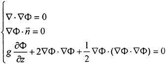
(1)
which hold into the fluid domain, on the hull and on the free surface respectively. The total velocity potential is assumed as the sum of a double body potential ΦD and of a wavy potential which is considered of a smaller order of magnitude. In addition, all the relevant terms into the non linear free surface equation are expanded in Taylor series in the neighborhood of the plane z=0. On this basis, a linearization of the free surface results in the following formula:
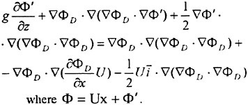
(2)
Coherently with an indirect boundary element methodology, the induced velocities at a field point P are given in terms of a source distribution on the boundary hull and undisturbed free surfaces SH and SF according to the following formula:
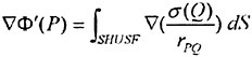
(3)
which is approximated in terms of the sum of the contributions of a given number of quadrilateral panels.
Defining the induced velocities at a collocation point i by a quadrilateral j as:
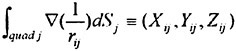
(4)
the discretised version of the linearised equations can be written:
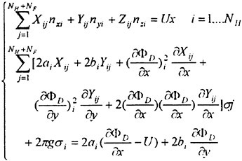
(5)
in which the terms ai and bi are so defined:
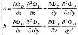
(6)
In addition to the customary pressure integration on the hull surface, the wave resistance can be determined by a transverse cut downstream the hull exploiting the methodology described in [7]. According to this reference, the resistance may be computed starting from the Fourier transform of a record of the wave pattern along a suitable line perpendicular to the waterline axis of symmetry. The wave resistance is given by the following formula:
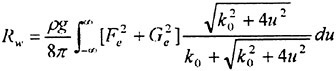
(7)
in which u is the transverse wave number, ![]() represents the free wave spectrum amplitude and k0=g/V2 is the fundamental wave number. Ā is directly linked to the Fourier transform of the wave heights along two transverse cuts or, alternatively, of the wave height and of its longitudinal slope along a single transverse cut.
represents the free wave spectrum amplitude and k0=g/V2 is the fundamental wave number. Ā is directly linked to the Fourier transform of the wave heights along two transverse cuts or, alternatively, of the wave height and of its longitudinal slope along a single transverse cut.
The motivation for the use of such methodology is twofold. Often, pressure integration is affected by numerical errors which arise in balancing large pressure forces in opposite directions, whereas, probably a more favourable situation exists in analysing wave records and in deriving the wave resistance from the integration of a positive quantity as the squared free wave spectrum. Furthermore a complete and quantitative definition of the wave pattern may be given by the free wave spectrum. In fact, numerical methods of this type are often employed in a preliminary design phase by looking at the wave pattern and the wave profiles along the hull rather than the wave resistance.
The free wave spectrum gives a more quantitative information because it allows to analyse the wave pattern and to associate its energy content to its wave transverse number or alternatively to its propagation angle.
This analysis is particularly useful for the validation of a numerical methodology because it allows to compare results in terms of spectral amplitudes giving more information about the predicted wave pattern. The relative position of the humps and hollows of the wave spectral amplitudes of the numerical and experimental methods can be examined adding further
and more complete requisites for a successful comparative application of a numerical methodology.
Of course, the possibility to carry out a sufficiently detailed analysis requires adequate definition of the free surface grid. This is easier into the field of high speed ships where higher fundamental wave numbers involve longer waves and, consequently, less panels for their definition.
In fact, indicating a typical width of the discretized free surface as βL, where L is the length of the vessel, and a typical panel width as Δy. here supposed as uniform, the Nyquist cut off transverse wave number will be:
(8)
It follows that with a given number Ν of uniformly distributed panels:
(9)
So, considering for instance a transverse strip of 30 uniformly distributed panels and β=1 it would result a maximum non dimensional wave number of about 5.9 for Fn=0.25 and 23.55 in case of Fn=0.5.
These figures correspond to a wave angle of 66° and 78° respectively. Though the wave spectral content is shifted toward higher wave number for high speeds, these values are already sufficient for a good definition, especially considering that the operative range of high speed vehicles is over Fn=0.5.
Similar considerations apply also in case of unequal transverse spacing of panels, which are often adopted in numerical Rankine source methodologies to better define the near field wave pattern, provided that reference is made to the largest width.
5. WAVE RESISTANCE EVALUATION WITH NUMERIC TRIM AND SINKAGE PREDICTIONS
The numerical method described so far has been extended to the case of high speed crafts, for which the dynamic sinkage and trim are, as known, very important [4]. In particular, rather than making the calculation for a fixed predetermined attitude, an iterative method has been developed in order to converge towards the dynamic trim and sinkage of the hull.
In general it consists in solving a simple nonlinear system of three equations (forces and moments in the vertical plane) in three unknowns (trim angle, sinkage and wave resistance) of the kind:
(10)
The problem becomes fairly simple and reduces to the naval architect well known static equilibrium of a floating body, when the dynamic forces and moments are neglected. The static problem can easily be solved with any non-linear systems solution technique, being the function Fstat and Mstat typically well behaved. The addition of the dynamic forces and moments on the hull, instead, complicates the solution by adding further nonlinear contributions which need to be numerically evaluated and may introduce some oscillatory components around the solution.
A Newton-Raphson approach with a line searching and backtracking algorithm has been used to increase the probability of convergence towards the solution. At the moment no other kind of solution algorithm has been used and an investigation on more efficient methods to reach the convergence is programmed.
As a first step, the potential flow calculation is performed for the hull with an initial guessed trim: usually the even keel, if no better guess is known, as is the case of this study. The dynamic sinkage force and trim moment on the hull are evaluated by integrating potential flow pressures over the hull surface panels at each step. The hydrostatic restoring forces and moments of the hull and, in case of transom sterns, the hydrostatic contributions to forces and moment due to the dry transom are calculated, as well.
Starting from the first complete run with the initial guess, the modified Newton-Raphson scheme is followed with a complete run for each step to solve the non-linear, implicit equations of the dynamic equilibrium of the hull in the vertical plane.
Each complete run, at a certain trim angle ![]() and sinkage S, needs a new representation of the hull surface by panels, a complete double model run, a new arrangement of panels on the free surface and a new run of the potential free surface flow solver. New panelling routines, capable to automatically generate surface meshes at each iteration, have been developed and interfaced with the main program. This main routine performs the iterative convergence of the non-linear system to the solution, collecting at each step the global parameters. Eventually, all the potential flow characteristics, such as velocities, pressures, hull stream lines, wave resistance and wave patterns, are saved for the final solution.
and sinkage S, needs a new representation of the hull surface by panels, a complete double model run, a new arrangement of panels on the free surface and a new run of the potential free surface flow solver. New panelling routines, capable to automatically generate surface meshes at each iteration, have been developed and interfaced with the main program. This main routine performs the iterative convergence of the non-linear system to the solution, collecting at each step the global parameters. Eventually, all the potential flow characteristics, such as velocities, pressures, hull stream lines, wave resistance and wave patterns, are saved for the final solution.
The procedure has been applied to two reference round bilge hulls up to very high speeds (Fn=1.0). One without transom—the Wigley hull—and the other with transom stern—presented in this paper—both in double configuration: isolated and in tandem with a separation s/L=0.3. The Wigley hull has been mathematically defined up to the waterline, while a cylindrical vertical extension over the waterline has been applied.
The characteristic of the transom round bilge hull together with the results of the calculations and their
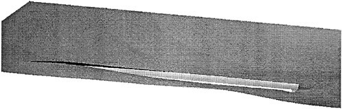
Fig. 4. Numeric 3D wave contour along the hull
discussion will be reported later in this paper.
Hereinafter, the general validation of the numerical method in the case of the Wigley hull forms, not tested for this paper, but taken from the available literature will be presented.
In general, an easy convergence of the method over the final dynamic attitude was shown during the calculations. In figure 5 an history of the dynamic trim and sinkage at FP, obtained for the Wigley hull at Fn=0.4 is plotted against the iteration number. As visible the final values are obtained after seven iteration starting from the initial even keel condition. For this calculation about 2700 panels were used in total over the hull and free surfaces and it took 4 hours to complete on a 266Mhz CPU speed computer.
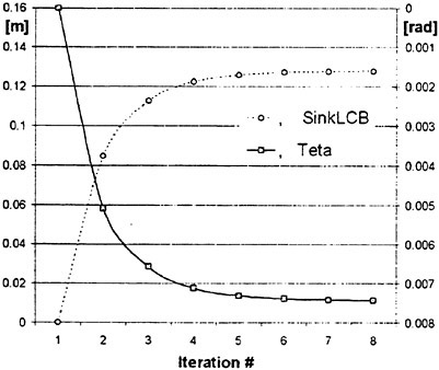
Figure 5—Convergence of dynamic trim and sinkage to equilibrium. Wigley hull at Fn=0.4.
One can play with the relaxation factor of the Newton step to possibly accelerate the convergence.
The presented wave resistance was calculated by the two method mentioned earlier, i.e. hull potential flow pressure integration and transverse wave cut.
A sensitivity analysis about the convergence of the results respect to the number of panels and type of panel distribution was made at a single velocity. One must require the stability of the predicted wave resistance, either in terms of Cw and in terms of predicted free wave spectra together with the convergence on the dynamic attitude. Roughly a minimum of about 300 panels over the hull and 2800 over the surface for the transom monohull were judged to be sufficient; these figures are modified to about 3200 over the surface and double the number over the hull, for the catamaran. For the Wigley simple hull even less panel can be sufficient for a stable wave resistance prediction.
The influence of the panel distribution over the predicted running trim and sinkage was made for the Wigley hull showing a sensibility of the method to these parameters, which must be chosen very carefully. An useful caution is to avoid abrupt changes in panel size between various zones such as, for instance, the transom wake and the adjacent free surface or between the hull and surface panels. For the catamarans it is important a good definition of the area between the twin hulls.
The result of the computation for the Wigley hull in isolation are shown in figure 6 and in tandem with a separation of s/L=0.3 in figure 7. The values of dynamic trim angle and sinkage at FP nondimensionalised respect to Lpp are plotted together with the wave resistance calculated with the two numerical methods.
The calculation were made over a wide range of Froude numbers starting from 0.3 to 0.8 and are compared with the experimental data available (Insel and Molland [12]. for catamaran and monohull at highest speeds and BHSC and Tokyo towing tanks for monohull). For sake of completeness together with the Cw experimental data also the CR values are presented.
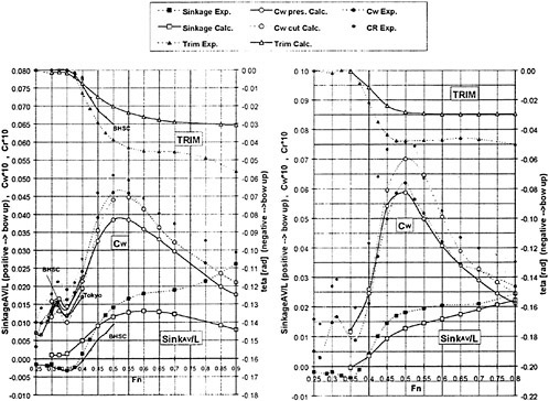
Figure 6—Wigley Monohull: Numeric wave resistance and dynamic trim and sinkage comparison with experiments
Figure 7—Wigley Catam.: Numeric wave resistance and dynamic trim and sinkage comparison with experiments
On the whole predicted curves of dynamic trim and sinkage show the same trend of the experimental ones and appear correctly fared, though the absolute values are underestimated. For the catamaran, the stabilisation on a constant trim angle for speed over Fn=0.5 is well reproduced. For the monohull the changes in slope of the trim angle over Fn=0.7 found in [12] is not followed. The scatter of the experimental data is of the same order of magnitude of that between the theoretical and experimental values.
Altogether, the predicted wave resistance agrees well with the measured one. As already found in the case of an application on NPL hulls [4] the wave resistance obtained by the transversal cut method seems better behaving than that calculated with pressure integration. For the lower speeds, though, to be accurate the former method requires a large number of panel in transversal direction, while pressure integration seems to suffer less of the relatively low panels number (Wigley monohull under Fn=0.4). The Froude numbers of the humps and hollows of the resistance curve are accurately predicted by the method.
The inaccuracy in predicting the running trim and sinkage may be caused by some non-linear aspects which were neglected in the formulation of the numerical method used. Among them perhaps the most important is that the hydrostatic hull forces and moments are calculated, at a certain velocity and attitude, respect to the undisturbed free surface, while it is believed that considering the actual wave contour along the hull for the calculation can give appreciable differences. As an example in figure 4 an isometric view of the wave contour along the hull is presented for the CAT1 catamaran at Fn=0.8. The hull surface visible in the figure was panellised by the program with the final trim and sinkage up to the undisturbed free surface plane, according to the linear condition.
Hence we suppose that the predicted dynamic attitude will be affected by this approximation, being the equilibrium condition evaluated by hull forces and
moments calculated not respect to the final wave contour along the hull, but for the undisturbed free surface level.
Interesting would be the verification of the improvement in the prevision of the dynamic attitude at high speeds achievable with the full non-linear condition, which is believed will grant better accuracy.
6. NUMERICAL AND EXPERIMENTAL RESULTS
For CAT1 the tests were carried out both on the catamaran with three different separation to length ratio s/L=0.225; 0.300; 0.375 and on its demihull in the Naples University towing tank.
The wave pattern resistance was obtained according to the multiple longitudinal cut method with reflections.
Figure 8 shows versus Froude number, for both the demihull and two separation ratios of the catamaran, the residual resistance coefficient and a comparison between the experimental wave pattern resistance coefficient Cwp, with those calculated by integration of the pressure on the hull surface and by a numeric transverse cut by using the experimental values of sinkage and trim into the numerical calculations.
The comparison between the numerical method and the experimental wave pattern analysis has been also carried out in terms of wave patterns and of wave spectra. Examples of wave patterns comparison are given in figures 9 and examples of free wave spectra for three different Fn values for the monohull and the catamaran with s/L=0.300 separation ratio are shown in figure 10.
The results for the spectra are given in terms of ![]() . Both from the wave patterns and from the spectra an overall satisfactory agreement may be noted. In particular, from the spectra, the effect of the speed upon the generated waves is evidenced: the wave energy is progressively moved towards higher wave propagation angles. In addition, also the different distribution of the spectral content relative to the catamaran when compared with the demihull in isolation, due to wave interference effects, is clearly indicated. The numerical spectra manifest the same trend as those obtained from the experiments, though some shifts on the peaks are occasionally noted. They are also, in general, smoother, and this is probably due to the different wave number interval allowed by the experimental method.
. Both from the wave patterns and from the spectra an overall satisfactory agreement may be noted. In particular, from the spectra, the effect of the speed upon the generated waves is evidenced: the wave energy is progressively moved towards higher wave propagation angles. In addition, also the different distribution of the spectral content relative to the catamaran when compared with the demihull in isolation, due to wave interference effects, is clearly indicated. The numerical spectra manifest the same trend as those obtained from the experiments, though some shifts on the peaks are occasionally noted. They are also, in general, smoother, and this is probably due to the different wave number interval allowed by the experimental method.
For the monohull and the catamaran with s/L=0.3 the complete iterative numeric procedure was also used and the results are shown in the fig. 11 and 12.
As already mentioned, for the sake of physical congniency more than for a real numerical need, the contribution of the hydrostatic force and moment of the dry transom (which evidently loose the static pressure on its surface) has been taken into account at each iteration to verify the equilibrium in the vertical plane. This, contribution, as imagined, is of a secondary order of magnitude respect to the hydro static and dynamic forces and could be neglected.
A general good agreement in terms of trends is found especially for Fn∈[0.5, 0.8]. The predicted trim is overestimated for both configurations, on the contrary of what found for the Wigley hull. Also in this case, for the monohull, the experimental wave resistance is well followed by the calculated pressure integration resistance, while for the catamaran pressure integration is the inverse. The tendency of the experimental wave resistance to stabilise for Fn>0.8 is not followed by the calculations, most probably for the incorrect trim predicted at these speeds.
Some problems for the catamaran at Fn>0.95 were encountered and the method showed difficulty to reach the convergence.
For CAT2 examples of wave profiles and spectra are shown in fig. 13 and 14. In this case, the experimental wave analysis was carried out according to a single longitudinal cut method by means of one profile recorded by a single probe (alternatively placed at different transverse distances from the model).
For the lower Froude numbers experimental data were also available from the smaller towing tank of Trieste. The resistance coefficients (figures 15 and 16) show in general the same trend for all the curves, but in general, the comparison is less satisfactory than before. Some slight differences may be noted between the wave pattern resistance of the two towing tanks that do not seem to be reproduced by analogous differences in residuary resistance, they may be due to the different facilities and to the relative higher possibility of measurement random errors upon the wave records of the smaller tank or to scale effects.
The numerical method generally manifests the same trend of the other curves and, in the case of the monohull, the results obtained by the numerical cut appear reasonable whereas those deriving from the pressure integration are too high., especially at the lower speeds. In the case of the catamaran the numerical transverse cut analysis provides too high values at the higher Froude numbers. Some considerations may be done though a further deeper analysis must be carried out. For the first catamaran the Froude number referred to the transom immersion is larger than in this second case, and this fact causes, in this second case, an higher speed for the transom to be dry (this is an hypothesis that was everywhere assumed for the numerical computations).
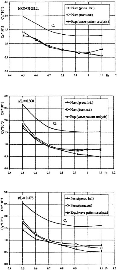
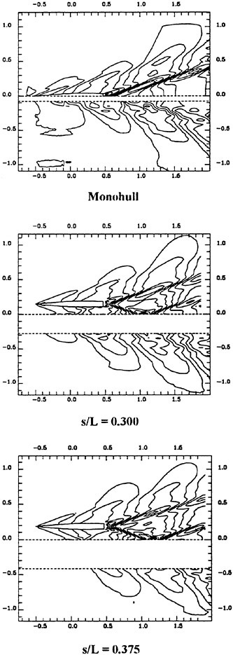
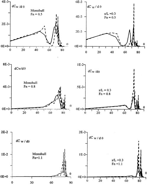
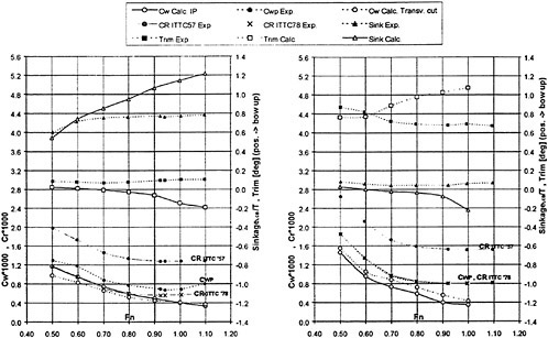
Figure 11—CAT1 monohull configuration: numeric trim, sinkage and wave resistance comparison with experiments.
Figure 12—CAT1 catamaran configuration: numeric trim, sinkage and wave resistance comparison with experiments.
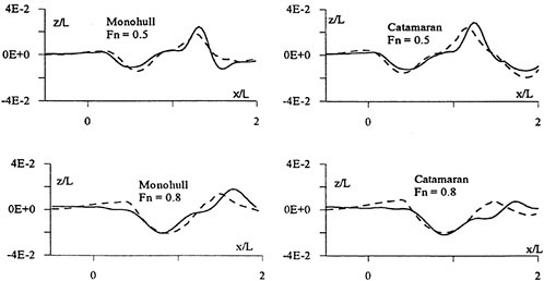
Figure 13: Examples of wave profiles for CAT2
Solid curve: numerical
Dotted curve: experimental
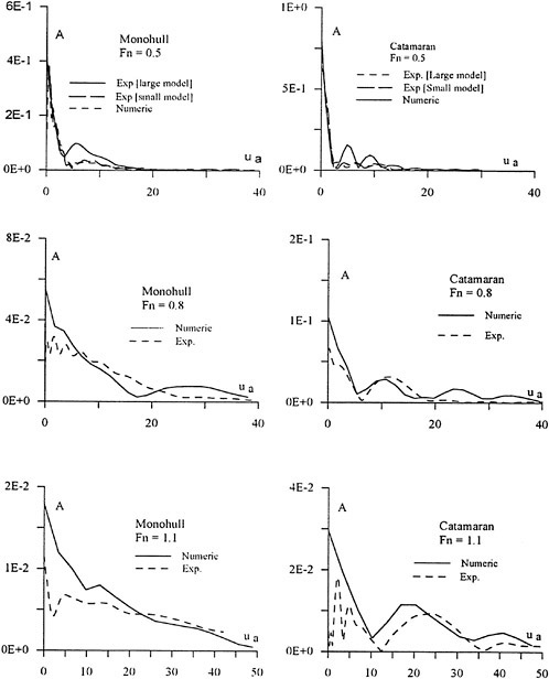
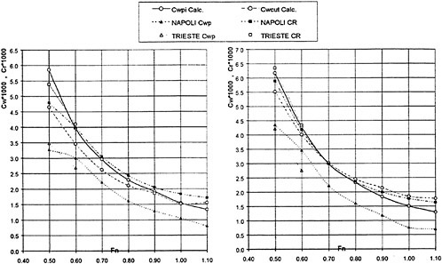
Figure 15—CAT2 Monohull: experimental/numerical wave resistance comparison
Figure 16—CAT2 Catamaran: experimental/numerical wave resistance comparison
Especially at the lower speeds, the wave resistance coefficient is for a large part composed of an hydrostatic term, so eventual errors on sinkage and trim have a non negligible effect on the resistance computed by pressure integration. At the higher Froude numbers the wave systems of the two demihulls of a catamaran are shifted downstream and are affected by the reflected waves of the truncated numerical domain. The wave interaction effects are in general quite complex to be entirely captured by the numerical method.
The first catamaran has lower volumetric coefficients relative to the length and results in finer forms, perhaps easier to be dealt with by a numerical method. The spectra of CAT2 deriving from the experimental pattern analysis in the two towing tanks. where they are available for the smaller one. appear quite similar as can be seen in figure 14. However, at Fn =0.5 a large difference can be noted between the numerical spectra and the experimental ones, that can probably be mainly attributed to a non completely dry transom. Finally, it should also be noted that the single longitudinal cut methodology manifests severe problems at high speeds due to the tank wall reflections.
For the hard chine monohull the wave pattern experimental analysis was performed by the single longitudinal cut procedure by using one probe adequately positioned both for the catamaran and for its demihull. Figure 17 gives the comparison among the residual resistance coefficients of the two geosims, the experimental wave pattern resistance coefficients and the numerical wave resistance obtained by a numerical transverse cut. The figure shows a significant difference between the numerical and the experimental results especially in the Froude number 0.4–0.6.
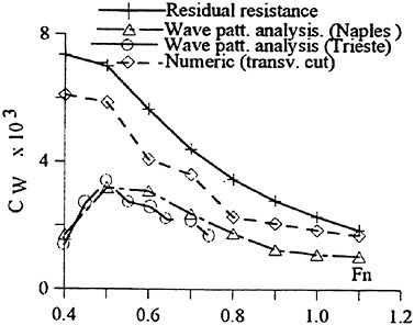
Figure 17: Demihull CAT2
However the difference on wave pattern resistance deriving by the two geosims are low. A better agreement of the numerical and experimental values can be noted at the higher Froude numbers. This result is confirmed by the comparison between numerical and experimental wave spectra represented in figure 18. The obtained results seem to show that the single longitudinal cut procedure is not adequate for the measurements of the wave resistance of high speed crafts. Overall, in the lower Froude range with the transom immerse, because of the wave energy which is not transferred into the measured wave profile.
The hard chine monohull is a vessel that poses several problems to be dealt with both by a numerical method and by an experimental wave pattern analysis. In fact, complex flow phenomena can be induced at the hard chine and, in addition, at very high speed some planning behaviour could be noted. Furthermore, the hull in question is fitted with a quite deep transom that was observed to become completely dry at Froude numbers close to 0.7. Both the numerically predicted and the experimental results from the wave pattern analysis are correctly lower than the residuary resistance, but the experimental wave pattern analysis results quite low. Some of the foregoing considerations about the second catamaran may be confirmed in this case. The wave system is influenced by the presence of the wetted transom with possibility of breaking waves and, consequently, low values of wave pattern resistance. This fact may be noted also looking at the wave spectrum at Fn=0.6 (fig. 18) in which the numerical method based on the hypothesis of a dry transom predict higher values of the spectral amplitudes resulting in a larger area of the spectrum and in a different trend. At the higher Froude numbers the trend of the curves seems to be the same but the numerical method continues to overpredict the spectral content.
7. CONCLUSIONS
Wave pattern analysis were performed for three different hull forms of high speed crafts by using different experimental and theoretical procedures in order to verify their reliability: some results are given in this paper. The most used experimental procedure of the single longitudinal cut for the wave analysis gives good results for traditional ships but for high speed crafts suffers of the short wave recording length . In this case the multiple longitudinal cut procedure with reflections gives better results as shown examining the results obtained from its application to the first catamaran CAT1 and those obtained for the catamaran CAT2 and for the monohull for which a single longitudinal cut was applied. The comparison between the experimental and numerical wave analysis shows a good agreement especially if the running trim and sinkage is correctly taken into account. The procedure presented in this paper for this aim gives good results for the Wigley hull form but it must be improved for usual hull forms of high speed crafts. The numerical transverse cut procedure seems to provide very interesting results, however this methodology must be also improved to be adopted for routine numerical wave pattern analysis of high speed crafts.
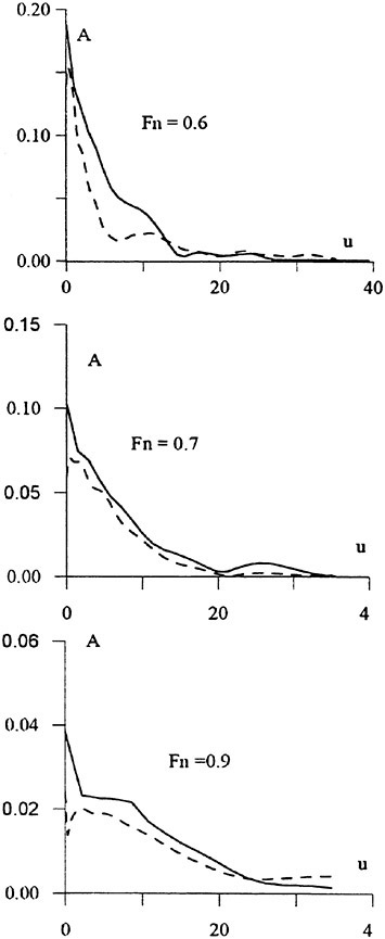
Figure 18: Examples of free wave spectra for the demihull CAT2
Solid curve: numerical Dotted curve: experimental
ACKNOWLEDGEMENTS
This work is part of a research supported by the Italian Ministry of University (MURST fondi ex 40%)
REFERENCES
1. Bruzzone D. “Numerical Evaluation of the Steady Free Surface Waves”. CFD Workshop Tokyo 1994. Ship Res. Inst., Tokyo. Vol 1. 1994, pp. 126–134.
2. Bruzzone D., Cassella P., Miranda S., Pensa C., Zotti I. “Steady Waves of Series 60 CB=0.7 Hull. Results and Experiments on Geosims.” Proceedings of the First Int. Conf. on Marine Industry, ed. P.A. Bogdanov, Varna, Vol I, 1996, pp. 59–73.
3. Bruzzone D., Cassella P., Miranda S., Pensa C., Zotti I. “Wave Patterns and Wave Resistance: Validation of a Numerical Method Using Geosim Experimental Results”. Proc. of the 2nd Int. Conf. on Hydrodynamics, Hong Kong. Vol. 1. 1996. pp. 127–132.
4. Brizzolara S., Bruzzone D., “Wave Resistance Evaluation for High Speed Vehicles”, Proceedings of High Speed Marine Vehicles International Conference, Sorrento, Italy, Vol. 1. 1997, pp. 3–12.
5. Bruzzone D., Cassella P., Pensa C., Scamardella A., Zotti I. “On the Hydrodynamic Characteristics of a High-Speed Catamaran With Round-Bilge Hull: Wave Resistance and Wave Pattern Experimental Tests and Numerical Calculations” Proc FAST ’97. Sydney Vol. 2, 1997, pp. 581–589.
6. Sharma S.D. (1966) “An Attempted Application of Wave Analysis Technique to Achieve Bow Wave Reduction” Proc. of th VI Symposium on Naval Hydrodynamics, Washington D.C., 1996 pp. ~731–773.
7. Eggers K.W.H.; Sharma S.D.; Ward W. “An Assessment of Some Experimental Methods for Determining the Wave making Characteristics of a Ship Form” ; TRANS. SNAME, Vol. 74, 1967, pp. 112–157.
8. Moran D.D., Landweber L. “A longitudinal Cut Method for Determining Wavemaking Resistance” Journal of Ship research. Vol. 16, N. 1, March 1972, pp. 21–40
9. Tsai C.E., Landweber L. “Further Development of a Procedure for Determination of Wave Resistance from Longitudinal-cut Surface-Profile Measurements”; Journal of Ship Research, vol. 19, n.2 June 1975, pp. 65–75.
10. Insel M. “An Investigation Into the Resistance Components of a High-Speed Displacement Catamaran”, Ph. D. Thesis; Department of Ship Science, University of Southampton, 1990.
11. N.Hogben “Automate Recording and Analysis of Wave Pattern Behind Towed Models” Trans. of The Royal Institute of Naval Architects, vol. 114, 1972, pp. 127–153.
12. Insel M., Molland A.F. “An Investigation Into The Resistance Components of High Speed Displacement Catamarans” Transactions of The Royal Institution of Naval Architects. Vol. 134, 1992, pp 1–20 .
Evaluation of Methods for Estimation of Extreme Nonlinear Ship Responses Based on Numerical Simulations and Model Tests
L.Adegeest, A.Braathen, T.Vada (Det Norske Veritas, Norway)
Abstract
In the present paper three different subjects are addressed: The first is to compare deterministic results for motions and global loads, obtained from experiments in a model basin, with results from a simulation program. The second is to show how limited information, in terms of transfer functions or relatively short non-linear time simulations, may be used in an optimum way to predict extreme values. Different existing methods are reviewed and the new Most Likely Extreme Response method is presented. The third is to estimate extreme values, based on the different methodologies presented under point two above, and to demonstrate the sensitivity of these extreme values to the methodologies chosen. The results are again compared with model test data.
1. INTRODUCTION
A number of research efforts are presently underway to improve the prediction of shiploads and motions. One example is the SWAN code (Kring et al [11]). This program exists at different levels of sophistication and is, at the most advanced level, based on large-amplitude 3-D time-domain solution with forward vessel speed. The implementation of non-linear effects varies within the different versions of the code. At present, no fully nonlinear code is available to the industry.
A review of available methods is given by Beck et al [5]. These types of codes make it possible to simulate the non-linear response of a ship in a specified seastate. Most often however, it is the estimation of the statistical properties of the response, which is of practical interest and not the results from the deterministic simulation of a limited duration ship response history as such. It is therefore important to have a well-funded strategy for how to use the results available from the new generation of non-linear ship wave analysis programs in order to obtain statistical statements from deterministic simulations. In particular, extreme value estimates can be hard to obtain with sufficient accuracy. A straightforward method to obtain predictions of extreme values of the response would be to carry out simulations with a sufficiently long duration and to estimate the extreme values directly from the simulated record. Several well-known alternatives exist, based on this approach. Most commonly, a global statistical model is fitted to the entire response history, by either fitting a Hermite model to the first four moments of the response history (Winterstein [17]) or by fitting a Weibull model to the local maxima (Karunakaran [10], Winterstein and Torhaug [18]). Based on this information of the response process, extrapolation to the response level of interest is carried out. Alternatively one might use tail-fit models to predict extreme response levels by either fitting a Gumbel model to the largest peaks within a number of sub-intervals of the response history or by only using peaks over a certain threshold in the fitting of a Weibull model. (Winterstein and Kleiven [19], Mørk and Bitner-Gregersen [13], Maes [12]).
However, due to the large computer resources needed by the non-linear simulation programs at the most advanced level, it is not practical, from an engineering point of view, to carry out sufficiently long simulations to directly obtain accurate extreme value estimates. In particular, it may be extremely difficult to obtain long-term extreme value statistics by this “direct” approach.
The problem in question can be illustrated by the following example:
Several computer codes are available, based on strip theory including some non-linear effects. One example is the NV1418 code (Børresen and Tellsgård [6]). By using this program, it is possible to generate very long records of the ship response in a given irregular seastate. Consequently, even if the response in this case may be quite non-linear (and therefore non-Gaussian), it is possible to come up with response estimates with very small statistical uncertainty.
On the other hand, since the physical and numerical hydrodynamic model used by NV1418 is rather crude, the model uncertainty will be significant. Consequently, the uncertainty associated with the raw data (i.e. the simulated records) which are the basis for the response estimates will also be significant.
Due to this, the total uncertainty (which is a function of both statistical and model uncertainty) can be large. If we use the much more advanced non-linear computer program SWAN however, we have reason to believe that the model uncertainty is significantly smaller. However, since it is (at present) only feasible to generate relatively short records of the ship response, it is inevitable that the statistical uncertainty will be large. Hence, if used uncritically, the engineer may end up in a situation where the statistical uncertainty can offset the improvement in non-linear simulations.
One way to avoid this situation is to have a well-funded strategy for the selection of the wave-input to the simulations. For the engineer, the problem is to find the right compromise between simulation time (computer costs) and accuracy of the results. This means that a sound engineering method should be able to quantify the uncertainty associated with the reduction of simulation time.
The present paper will focus on the prediction of extreme values, based on the selective use of nonlinear time domain codes. Different methods will be reviewed and applied to vertical hull girder bending moments and shear forces. A new method based on the Most Likely Wave approach is presented. The methods are based on the assumption that the basic physics are included in the linear model, in the sense that large values of the linear response correspond to large values of the non-linear response when the waves in the two simulations are the same. The methods are illustrated using a monohull and a trimaran as examples.
2. THE COMPUTER PROGRAM SWAN-2 (DNV VERSION)
The computer program SWAN-2 is a 3-dimensional time domain program for arbitrary shaped ships (including multi-hulls) or other marine structures in waves. The ship may have an arbitrary forward speed, the waves can come from any direction and the responses can be computed in all six degrees of freedom. The program is based on a three-dimensional Rankine Panel method (Kring et al [11]). Radiation conditions are treated by including a zone where the free surface condition is modified such that the waves are absorbed, i.e. a numerical beach.
SWAN was originally developed in a cooperation between MIT and DNV, and versions have been developed further by both DNV and MIT.
SWAN-2 is, in light of the complex problem it solves, a very efficient program. Thus time records of a duration of several hours can be obtained with reasonable computational effort. It also benefits from extensive numerical stability analyses done in the early development phase (Vada and Nakos [16]). For this reason the stability is under good control and the program has become very robust.
The applied version of SWAN can be run in both a fully linear mode and in a non-linear mode. The transfer functions are derived from linear computations by Fourier analysis. The implemented non-linear option still solves the linear radiation and diffraction problem. All other effects are treated in a fully non-linear way. Important non-linear effects included are:
-
hydrostatics
-
Froude-Krylov force
-
inertia and gravity effects
-
water on deck
-
roll damping
The included non-linearities can give very significant contributions to both global loads and motions in large waves. This means that the non-linear simulations can differ considerably from linear simulations in such waves and thus be a very good indicator of the applicability of the different approaches described in this paper.
The SWAN-2 computations are strictly deterministic. Time records can only be obtained for a limited number of realizations of a given sea state. So despite the fairly good efficiency it is still necessary to combine those simulations with other methods to maximize the benefit.
This paper shows different ways of doing this. These statistical methods will be even more important if more advanced non-linear simulations are to be carried out (SWAN-3). Such simulations might be necessary in extreme waves and they are approximately two orders of magnitude more time consuming than the simulations we have carried out. For the purpose of this paper, SWAN-2 is a very useful tool and all the simulations used in this paper have been carried out with this program in either linear or non-linear mode. In the following, the program will simply be referred to as SWAN.
3. METHODS TO CALCULATE EXTREME RESPONSES
The extreme value prediction methods, presented in this section, are all candidates to be used in combination with a non-linear time domain program. Methods, which would require the generation of long time histories to give converged estimates of extremes, are not discussed here. In the examples however, presented in section 4, some of those methods will be applied to illustrate the statistical uncertainty of the extremes obtained.
3.1 Regular design wave
This method is the simplest method to use and can be considered as a standard engineering tool. The following steps are involved in determining the design wave:
-
Calculate the long-term extreme value based on standard methods, assuming linear theory.
-
The period of the design wave (for a given response, point on the structure, wave heading, vessel speed, etc.) may be chosen as the period corresponding to the peak of the transfer function.
-
The amplitude of the design wave is obtained by dividing the extreme value, obtained from long term statistics, by the value of the transfer function at the period found above. If the amplitude comes in conflict with steepness limits, corrections have to be made on amplitude and/or period.
-
When the design wave is found, it can be used as input to a non-linear simulation. The resulting response is then taken as the extreme value estimate.
The design wave may be a questionable representation of the actual wave loading: In real life, the actual “wave-event” which gives the maximum response at a given point on the structure during it’s life time will certainly be different from the design wave.
3.2 Critical Wave Episodes
This method is based on the assumption that it is possible to identify short segments (typically a few wave cycles long) of wave input which are likely candidates to produce extreme responses. Such wave segments are denoted Critical Wave Episodes (CWE) (Torhaug, Winterstein and Braathen [14]). The critical wave episodes are then used as input to a number of short nonlinear simulations.
The identification of the critical wave episodes must be based on a priori knowledge about how the vessel behaves in waves at different speeds and wave directions. Very long realisations of the linear ship behaviour can be obtained relatively easy and inexpensive if a complete set of transfer functions for ship motions and loads is available. Therefore, these transfer functions are calculated first and used, implicitly, as a basis for the selection of critical wave episodes. It should be noted however, that additional information about the ship behaviour in waves, not contained in the transfer functions, could in principle be utilised in the selection process. It is also possible to identify critical wave episodes directly from simulated realisations of the surface elevation, if some main properties of the response process are known. For instance, wave episodes with wavelengths close to the ship length and wave heights above some specified level, may well serve as candidates for critical wave episodes, if the relevant response is mid ship bending moment. However, it has been shown in practice, that in this case, identification based on linear ship response is the best alternative.
In order to estimate some desired statistics; e.g. mean, median, 75% fractile etc in a given storm, a given number of nH realisations of that storm have to be simulated in terms of wave input time histories. Within each realisation, nE critical wave episodes may be identified. Each critical wave episode will have a certain duration nC, measured in terms of number of wave cycles. This duration has to be sufficiently long so that both transients in the simulation and memory effects are accounted for.
If the problem is to estimate the extreme response during a typical storm with a given duration, the necessary simulation time (costs) will be proportional to the product of nH, nE and nC. If we treat this product as a constant, an optimum choice of the individual factors will exist, for a given type of response. An engineering method, based on the critical wave episode approach, will have to include recommendations for such an optimum choice.
Torhaug, Winterstein and Braathen [14] showed that, for the midship vertical bending moment of a mono hull with a large flare, typically 36 wave cycles (nH·nE·nC) will be sufficient to estimate the hourly maximum bending moment with approximately 5% error.
3.3 Most Likely Extreme Responses
The objectives of the Most Likely Extreme Response method development were to take into account the correct response memory effects and to reduce the number of uncertain variables, which are to be input to an extreme response analysis. The use of non-linear time domain programs had to be limited at the same time.
The theory that was used to generate Most Likely Wave (MLW) profiles with conditioned amplitude (Tromans et al [15]) and frequency (Friis Hansen and Nielsen [8]) has been applied to response spectra. Using the amplitude and phase information of the frequency response functions, it is possible to derive the irregular wave train, which caused the linear Most Likely Extreme Response. Successively, non-linear simulations can be carried out with this irregular wave train as input. The procedure has
been described and tested for the estimate of extreme vertical bending moments and maximum water heights on deck by Adegeest, Braathen and Løseth [3]. A brief review of the method is given below.
Definition of waves
In SWAN, the wave surface is defined by a linear superposition of Ν regular wave components with different amplitudes, frequencies, headings and phases as follows:
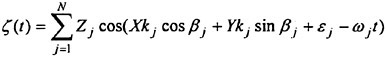
where X and Υ are the earth-fixed coordinates in which the wave elevation is calculated, k is the deep water wave number, defined as k=ω2/g. The wave heading β is defined as 180° in head waves. Each wave component with frequency ω results in a response component with encounter frequency ωe. The relation between the wave frequency and encounter frequency for a vessel travelling along the line Y=0 is given by:
where U is the mean forward speed of the vessel. It follows that the wave surface elevation in the origin of the mean ship-fixed system is defined as
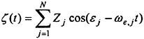
Calculation of Most Likely Extreme Responses
After calculating the frequency response function, the response spectrum can be calculated for the design seastate according to Syy(ω)=|Η(ω)|2 Sςς(ω). Before applying the MLW-procedures to the response spectrum, the spectrum has to be transformed to a frequency of encounter basis as follows:
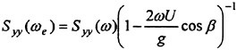
A random set of response amplitudes and phases, or in-phase and out-phase components, can be generated at a discrete number of Ν frequencies, such that:
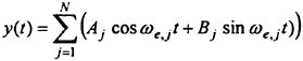
Aj and Bj are independent standard normal distributed variables having zero mean and an expected value for the squares equal to
Transformation of these Gaussian variables to a phase angle and an amplitude leads to a uniform distribution for the phase angle and a Rayleigh distribution of the amplitude Yj with
After determination of the random response components Aj and Bj, the components can be conditioned such that at time t=0, the random response has the prescribed linear ULS amplitude and frequency. In the present study, the statistically expected frequency, which is equal to the mean frequency ω*=m1/m0, was used. Conditioning of the response components is achieved by applying the theory of the Most Likely Wave model. The output of this conditioning process is a set of modified Aj’s and Bj’s, Aj* and Bj*. Note that both random conditioned sets of response components can be generated as well as the Most Likely Extreme Response, i.e. the set of components giving the mean response.
Derivation of the underlying wave profile
The last step in the procedure is to derive the underlying wave profile, which caused the Most Likely Extreme Response time series according to linear theory. This is achieved using the frequency response functions, which were already calculated using SWAN in its linear mode. For each frequency of encounter, present in the response signal, the amplitude Zj of the incoming j-th wave component with frequency ωj is derived according to
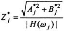
The phase εj of the j-th wave component is derived from
where φ is the phase angle of the frequency response function at frequency ω. Finally, the underlying conditioned wave profile in the earth-fixed reference frame is defined by:
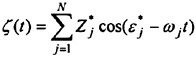
This wave profile will result in the linear Most Likely Extreme Response with specified amplitude and frequency at time t=0. By modifying the phases properly, another set of wave components is found which defines the same wave profile in space, but delayed in time such that at time t=tamx, the response obtains the specified magnitude and frequency. This allows a nonlinear inswing into the Most Likely Extreme Response without transient effects, induced at the start of the simulation.
Nonlinear SWAN simulations
After calculation of the set of wave components inducing a linear conditioned random or Most Likely Extreme Response, SWAN can be run in its non-linear mode to calculate the Most Likely Extreme Response including non-linear effects, i.e. the final ULS value. Linear and non-linear results can directly be compared in the time domain and non-linear correction factors are easily derived. A typical simulation length in irregular waves is accordingly reduced to 5–10 response cycles. This is comparable with the typical number of response cycles in critical response episodes selected from unconditional randomly generated time traces (Torhaug et al [14]).
4. RESULTS
4.1 Example 1: Container vessel ‘Snowdrift’
The purpose of the analyses, described in this first example, is to demonstrate the application of different methods for the prediction of extremes and to verify the results against model test data. The procedures applied are not Ultimate Limit State procedures rather than a short-term statistical analysis of one particular seastate.
Model tests
Use is made of a set of model tests, which were performed as part of a co-operative research project. The project was focused on investigation of sag/hog ratios in slender vessels. The ‘Snowdrift’-model was build as a back-bone model with three segments, allowing the measurement of global loads amidship (station 10) and at a quarter of the length aft of the fore perpendicular (station 15). The main particulars of the ‘Snowdrift’ are summarized in Table 1. Figure 1 shows the under-water part of the vessel as modeled in SWAN.
Table 1 Main particulars of the ‘Snowdrift’.
|
Length between pp |
160.0 m |
|
Breadth |
24.65 m |
|
Draft |
8.93 m |
|
Displacement |
20491 tonnes |
|
Block coefficient |
0.57 |
|
Waterplane are coefficient |
0.71 |
|
Pitch radius of gyration |
39.39 m |
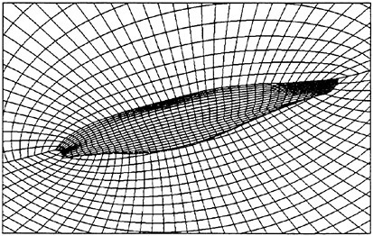
Figure 1 SWAN panel distribution of the ‘Snowdrift’ at a draft of 9.0 meter, including free surface discretization.
The model tests were performed in regular waves over a range of frequencies and wave amplitudes, and in irregular waves. Measurements in irregular waves were performed only for 1500 seconds on full scale. The wave spectrum, realised in the model basin, is presented in Figure 2. Characteristics of the wave spectrum are Hs=4.8 meter and Tz=8.0 seconds. The same spectrum has been used in all the irregular wave analyses as described below. In this particular run, the measured maximum midship sagging and hogging bending moment were respectively 4.46·105 kNm and −2.31·105 kNm. These values have been collected in Table 3. The measured mean response period was 6.7 s.
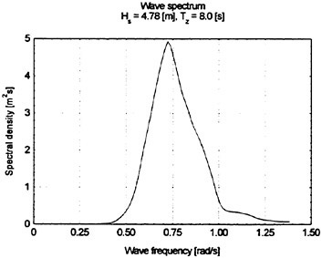
Figure 2 Wave spectrum as measured in the irregular wave experiments for the ‘Snowdrift’, and as used in the irregular wave SWAN analyses.
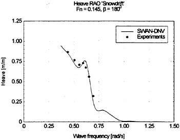
Figure 3 Heave RAO for the Snowdrift at Fn=0.145 in headwaves.
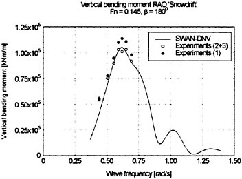
Figure 4 Vertical bending moment RAO (station 10) at Fn=0.145 in head waves.
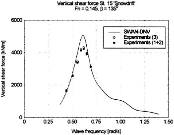
Figure 5 Vertical shear force RAO (station 15) for the Snowdrift at Fn=0.145 in head waves.
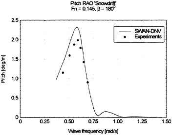
Figure 6 Pitch RAO for the Snowdrift at Fn=0.145 in head waves.
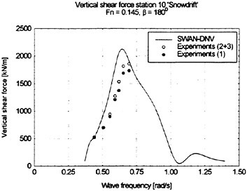
Figure 7 Vertical shear force RAO (station 10) for the Snowdrift at Fn=0.145 in head waves.
Linear transfer functions
Figure 3–Figure 7 show the measured and calculated transfer functions for heave, pitch, midship vertical bending moment and shear forces amidship and at a quarter of the length aft from the bow. The experimental hull girder loads were derived from the measured forces on the backbone plus inertia effects. The integrations were performed from bow to stern and from stern to bow. These results were not identical, indicating an inconsistency in the mass distribution. Taking into account these uncertainties in the mass distribution of the towing tank model (a mass moment of inertia was reported for the section between station 10 and 15 which was only realisable with two (unequal) mass points at maximum distance), a good agreement was found between the measurements and the simulations.
Linear extreme estimate using Rayleigh distribution
The first estimate of the extreme response in the 1500 seconds sea state is made according to linear theory. The expected linear extreme value is calculated using narrow band short-term statistics. The midship bending moment response spectrum is calculated on the basis of frequency of encounter using the transfer function in head waves, Figure 4, in combination with the measured wave spectrum, Figure 2. At first, the mean response encounter period is calculated from the response spectral moments according to Tmean= =2πm0/m1. The expected number of oscillations n is found by dividing the exposure period (1500 seconds) by the mean response period. Successively, the expected extreme value is calculated by cutting the Rayleigh distribution at probability level 1/n. This resulted in a mean response period equal 6.4 seconds (234 response cycles) and an expected linear extreme bending moment equal 3.17·105 kNm This result is also presented in Table 3.
Nonlinear simulations in random irregular waves
A straightforward method to obtain an estimate for the nonlinear maximum midship vertical bending moment in irregular waves, is to perform ‘enough’ nonlinear simulations in irregular waves and to identify the realized extreme response from the simulated time histories. Questions are how many response cycles have to be simulated to obtain a statistically reliable estimate and how large is the uncertainty of the extreme which finally has been realized. These topics were investigated by Torhaug, Winterstein and Braathen [14].
For the current paper, only one long nonlinear SWAN simulation in random irregular waves has been performed. A deterministic wave amplitude distribution has been used, whereas the phases are randomly uniform distributed between [0,2π]. This procedure guaranteed an exact representation of the spectral properties of the measured waves by the simulations program. It was not possible, however, to reproduce the exact wave history since these data were not available in digital form. Therefore, it cannot be expected that the calculated extreme value will match well with the measured extreme since this would require the input of the exact wave profile. The simulated results can only be considered as an approximation, and are affected by statistical uncertainty.
By running SWAN in its nonlinear mode, an extreme midship sagging moment of 4.81·105 kNm was found. In hogging, an extreme value of −2.17·105 kNm was found. These values have also been collected in Table 3.
Regular design wave analysis
Normally, the regular design wave approach is applied to obtain nonlinear corrections to the calculated linear ULS value. In this section, the method is used in its unmodified form to compute a nonlinear correction in a short-term condition. The purpose of the analysis is to illustrate the sensitivity of the nonlinear corrections to the wave frequency. Following the procedure, the wave frequency was chosen to be equal to the peak frequency of the vertical bending moment transfer function. The wave amplitude was derived by calculating the expected extreme linear response in the particular 1500-second sea state, and dividing this value by the transfer function value at the peak frequency. This procedure results in a characteristic wave with the following properties: period Τ=10.1 s, amplitude a=3.02 m. In order to investigate the sensitivity of the nonlinear corrections around this frequency, a slightly shorter and longer wave have been analyzed, both with modified amplitudes, such that the resulting linear response is equal to the expected linear extreme of 3.17·105 kNm. These waves are respectively characterized by T=9.6 s, a=3.18 m and T=10.6 s, a=3.11 m. The resulting maximum midship sagging and hogging bending moments are collected in Table 3.
Application of a moment-based Hermite model
Using the statistical moments, as calculated from the SWAN simulation in irregular waves, a Hermite moment-based model has been applied to calculate the probability density of extremes. The original formulations of the Hermite moment based statistical model were presented by Winterstein [17].
The realized first four statistical moments were equal to mean 1.88·105 kNm, standard deviation 9.27·105 kNm, skewness 0.880 and kurtosis 3.880. The length of the time history was 30000 samples. The variation of the statistical parameters within the simulated time history was large, indicating the importance of long time series in order to obtain converged parameters. To illustrate this, the mean, standard deviation, skewness and kurtosis were calculated in blocks of 10000 samples. The results are presented in Table 2.
Table 2 Realized statistical moments in three successive data blocks of 10000 samples of a simulation with a total length of 30000 samples.
|
Parameter |
Block 1 |
Block 2 |
Block 3 |
|
Mean [kNm] |
2.16·105 |
1.66·105 |
1.86·105 |
|
Stand.dev. [kNm] |
10.2·105 |
8.2·105 |
9.2·105 |
|
Skewness [-] |
0.68 |
0.43 |
0.52 |
|
Kurtosis [-] |
4.22 |
3.25 |
3.35 |
The expected extreme response has been calculated according to the Hermite moment model using the different sets of statistical moments. This required the specification of a probability level for the extreme response. This level is equal to 1/(expected total number of extremes), where the total number of extremes was already calculated to be equal to 234.
Figure 8 shows the calculated probability distributions of the extreme vertical bending moment (positive for sagging, negative for hogging). The measured distributions are plotted in the same Figure. A very good agreement is obtained between the measured distribution and the Hermite distribution, based on the statistical moments valid for the complete time series. But, the uncertainty in the results is large regarding the large scatter in predicted extremes when applying the three different sets of coefficients for the different data blocks. The realised extreme sagging and hogging moments, according to the Hermite model, are also collected in Table 3.
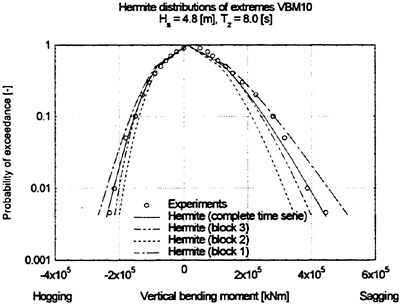
Figure 8 Calculated Hermite distributions of extreme midship vertical bending moment using different sets of statistical moments, compared with experiments.
MLER calculations
The last method which is illustrated here, is the Most Likely Extreme Response method. The procedure for conditioning of the response profile and derivation of the underlying wave profile has been outlined in section 3.3.
Two wave profiles have been derived: one profile producing the maximum positive extreme vertical bending moment after 100 seconds simulation (maximum sagging) and a second profile, resulting in the maximum negative vertical bending moment after 100 seconds simulation (maximum hogging). Nonlinear SWAN simulations in the two generated wave profiles finally resulted in the Most Likely Extreme sagging moment and the Most Likely Extreme hogging moment in this particular sea state for an exposure period of 1500 seconds. Time histories of the Most Likely Extreme sagging and hogging moment, as well as the underlying wave profiles, are shown in Figure 9 and Figure 10.
The simulated extremes are collected in Table 3. Figure 11 shows the same information as ratios of the calculated and measured extreme hogging and sagging moment.
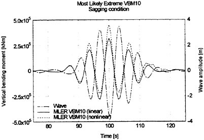
Figure 9 Histories of the linear and nonlinear Most Likely Extreme midship vertical bending moment in the ‘Snowdrift’ and of the underlying wave profile (sagging condition with conditioned linear positive extreme equal 3.17·105 kNm and mean response frequency).
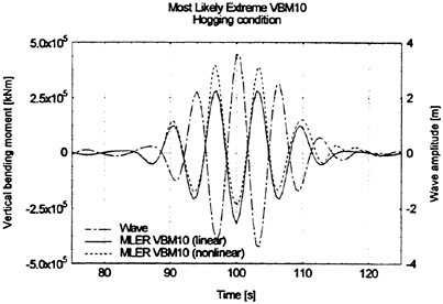
Figure 10 Histories of the linear and nonlinear Most Likely Extreme midship vertical bending moment in the ‘Snowdrift’ and of the underlying wave profile (hogging condition with conditioned linear negative extreme equal −3.17·105 kNm and mean response frequency).
Table 3 Measured and calculated extremes in the 1500 seconds sea state for the Snowdrift at Fn=0.145 in head waves (Hs=4.8 m, Tz=8.0 s).
|
Method: |
Maximum Midship sagging [kNm] |
Maximum Midship hogging [kNm] |
|
Measurements: |
4.46·105 |
−2.31·105 |
|
Rayleigh, linear: |
3.17·105 |
−3.17·105 |
|
Nonlinear simulation in random irregular waves: |
4.81·105 |
−2.17·105 |
|
Nonlinear simulation in regular ‘design wave’: |
|
|
|
1) T=9.6 s, a=3.18 m |
6.62·105 |
−1.53·105 |
|
2) T=10.1 s, a=3.02 m |
7.73·105 |
−1.10·105 |
|
3) T=10.6 s, a=3.11 m |
7.79·105 |
−1.65·105 |
|
Hermite moment model using simulated statistical moments based on statistical moments of |
|
|
|
1) Complete time series |
4.46·105 |
−2.41·105 |
|
2) Data block 1 |
5.13·105 |
−2.67·105 |
|
3) Data block 2 |
3.45·105 |
−2.01·105 |
|
4) Data block 3 |
3.99–105 |
−2.15–105 |
|
Nonlinear simulation of Most Likely Extreme Response: |
4.57·105 |
−2.36·105 |
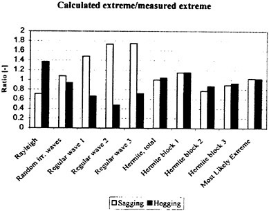
Figure 11 Ratios of calculated midship sagging and hogging moments over measured values for the Snowdrift.
4.2 Example 2: Trimaran
The purpose of the calculations in this second example is to demonstrate how SWAN can be used to calculate motions and loads on a multihull in both head and oblique waves. In Figure 12, a panel model of a trimaran is shown. Model test data for the vessel were not available at the time when the present article was written. The superstructure, including a wet deck connecting the two outriggers to the main hull, is not included in the figure. Under certain wave conditions, part of this wet deck may be submerged. This is not accounted for in the present calculations. Future versions of SWAN will be able to include such effects, and also slamming.
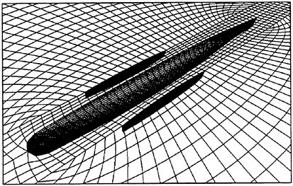
Figure 12 SWAN panel distribution of the trimaran, including free surface discretization.
Results from linear calculations, which are the basis for the statistical methods presented in the present paper, are presented in Figure 13 to Figure 20. The variation of the RAO’s for relatively short waves, most pronounced for the splitting moment in bow quartering waves, should be noted. This is due to the complicated shape of the hull, where for instance one outrigger can be close to a wave crest, and the other close to a wave trough. Interaction effects between the hulls are also contributing to the variation of the RAO’s for short waves.
The regular design wave approach and the Most Likely Extreme Response approach have been used to calculate ULS-values of the vertical shear force at a quarter of the length from the aft perpendicular, and the midship vertical bending moment. In the regular design wave approach, an amplitude of 10 m and a wave period of 9.5 s was used. The results are presented in Table 4 and in the Figures 21 to 25.
It is observed that both methods, for this particular case, gave quite similar results. It is also observed, from Figure 21, that the hogging moment for the design wave is largely reduced compared to the ULS-value predicted by linear theory. In the present case, the wave period and amplitude of the design wave are within a range where the effect of water on deck will be substantial. Therefore, the sag moment is also reduced compared to the linear predictions. This is demonstrated in Figure 21. For the larger waves, the time histories of the simulated nonlinear bending moments have a flat shape around the peak values. For instance, the increase in bending moment when the wave height is increased from 8 m to 10 m is very small.
In situations where there is no or little water on deck, the sag predicted by non-linear calculations is larger than the sag predicted by linear theory. In Figure 22, the “saturation effect”, in both sag and hog, is demonstrated.
Table 4 Simulated ULS values for vertical bending moment and shear force in the trimaran (5 knots, head waves).
|
Method: |
Midship vertical bending moment [kNm] |
Vertical shear force [kN] |
|
Linear ULS |
7.45–105 |
1.55·104 |
|
Regular design wave |
6.41·105 |
1.47·104 |
|
Most Likely Extreme Response |
6.73·105 |
1.51·104 |
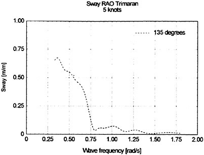
Figure 13 Sway RAO for the trimaran at 5 knots, in bow quartering waves (135°).
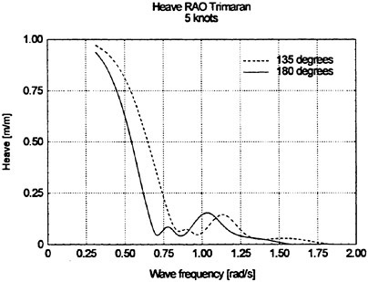
Figure 14 Heave RAO for the trimaran at 5 knots, in head waves (180°) and bow quartering waves (135°).
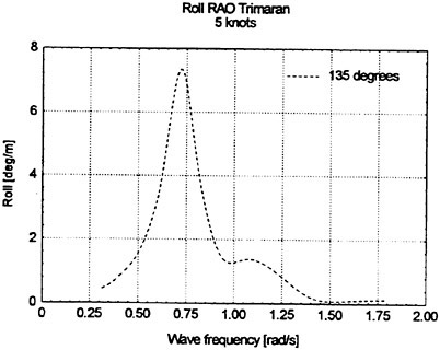
Figure 15 Roll RAO for the trimaran at 5 knots, in bow quartering waves (135°).
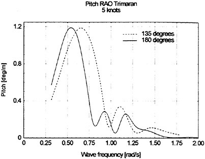
Figure 16 Pitch RAO for the trimaran at 5 knots, in head waves (180°) and bow quartering waves (135°).
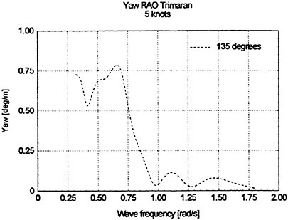
Figure 17 Yaw RAO for the trimaran at 5 knots, in bow quartering waves (135°).
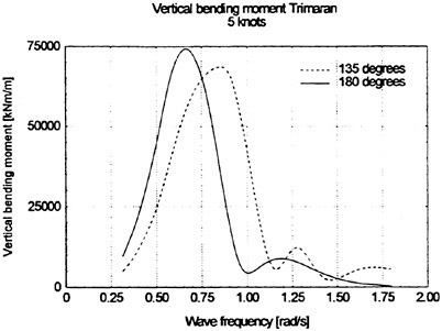
Figure 18 Vertical bending moment RAO for the trimaran at 5 knots, in head waves (180°) and bow quartering waves (135°).
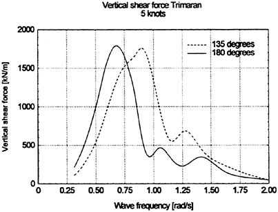
Figure 19 Vertical shear force RAO for the trimaran at 5 knots, in head waves (180°) and bow quartering waves (135°)
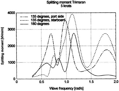
Figure 20 Splitting moment RAO for the trimaran at 5 knots, in head waves (180°) and bow quartering waves (135°).
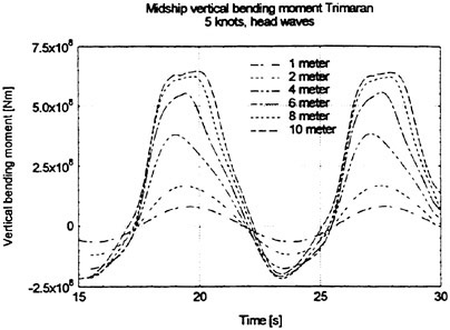
Figure 21 Snapshots of simulated vertical bending moments in regular waves (period 9.5 s) with different amplitudes for the trimaran (5 knots, head waves).
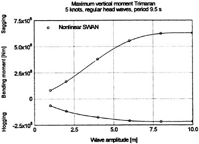
Figure 22 Calculated maximum hogging and sagging moment in regular waves (period 9.5 s) with different amplitudes for the trimaran (5 knots, head waves).
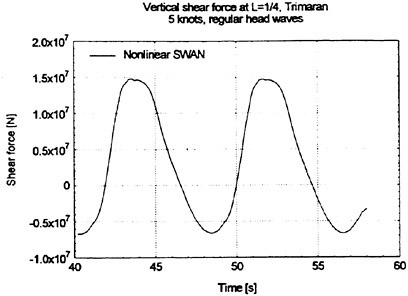
Figure 23 Snapshot of simulated nonlinear vertical shear force in regular waves (period 9.5 s, amplitude 10.0 m) (5 knots, head waves).
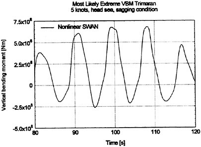
Figure 24 Simulated nonlinear Most Likely Extreme Response history for the midship vertical bending moment in the trimaran (5 knots, head waves).
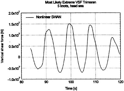
Figure 25 Simulated nonlinear Most Likely Extreme Response history for the vertical shear in the trimaran (5 knots, head waves).
5. DISCUSSION OF THE RESULTS
Different methods with different uncertainties were used to calculate the nonlinear extreme response in irregular waves. All the presented methods were based on the use of linear results to focus the nonlinear analysis. The successive nonlinear calculations were performed in relatively short time series, varying from 50 seconds to 1500 seconds real time. This was made possible by different modelings of the input waves, such as the regular design wave, the conditioned irregular wave causing the Most Likely Extreme Response and irregular random waves satisfying a specified spectrum. The results of the different applied statistical models were illustrated with two examples, both of them focused on the extreme vertical bending moment.
For the Snowdrift a rather complete set of model test data was available. A very good agreement was found between the measured distribution of extreme vertical midship bending moment and the Hermite distribution. However, the variations in the calculated tails of the distributions were large as a function of different sets of statistical moments. This variation implies that the extreme values, predicted by a Hermite model, are very sensitive to which part of the time traces is considered, which is a complication in the practical applicability of those types of models. In general, the extreme-predictions can be made with less uncertainty by simulating longer time histories, since the required statistical moments will become more stable. A possible solution to this convergence-problem is the calculation of the statistical moments in the frequency domain by using nonlinear transfer functions. The key-issue becomes the calculation of those transfer functions, which generally is a complicated issue. This procedure has been applied, amongst others, by Jensen and Pedersen [9] to the second order problem. Different solutions, up to the third order problem, were presented by Dalzell [7], Bendat [4] and Adegeest [1].
The regular design wave approach, as it has been applied in the ‘Snowdrift’ analyses, did not result in an accurate prediction of the extremes in the tested short term sea state. A better result could probably be obtained if other wave periods were used as critical waves. However, this immediately illustrates the sensitivity of the results to the selected wave period, which is not well defined in the regular design wave procedure for short term analyses.
An almost perfect agreement was found between the Most Likely Extreme Response method and the experiments. Important uncertainties, which have been removed in this approach, are the poorly-defined most critical period in irregular waves, response memory effects and the required simulation length. It should be
noted that the MLER approach can only produce one estimate at a particular probability level per simulation. In order to obtain more points on the probability distribution curve, different simulations have to be run with different wave inputs, derived from different conditioned responses.
For the trimaran, the results as obtained by the regular design wave approach and the Most Likely Extreme Response approach were very close.
6. CONCLUDING REMARKS
In this paper, it has been shown how extreme values can be estimated using a combination linear ship responses, short nonlinear time domain simulations and different statistical methods. Those types of statistical methods are of increasing importance when nonlinear time-domain programs are applied in direct calculations on a regular basis. It has been shown that the different methods can produce quite scattered estimates of the extreme responses in irregular waves compared with towing tank experiments.
The presented Most Likely Extreme Response method, which is based on application of the Most Likely Wave theory to response spectra, seems to be the most promising. Both when taking into account the obtained accuracy and the required simulation time. The accuracy of the calculated sagging and hogging extreme were both within 3% compared with model tests, whereas only 200 seconds of nonlinear simulations were required.
A major advantage of the method is, that the resulting extreme is the statistically correct product of well-defined quantities (a linear transfer function, a wave spectrum, the expected mean response period, the expected duration of exposure and the expected extreme value according to linear short term statistics). The only assumption that has been made, is that the extreme response, including all the nonlinear effects, is related in time to the extreme linear response.
In the future, fully non-linear methods will probably be available for engineering applications. Both the Most Likely Extreme Response (MLER) method and the Critical Wave Episode (CWE) method will benefit from this. In the MLER case, the required duration of the response simulation is so modest that an advanced fully non-linear program can be used directly. In the CWE case, a “hierarchic” approach may be adopted: application of a linear program first and a simplified nonlinear program in succession may do the identification of the critical wave episodes. This will reduce the number of episodes, which have to be analysed by the fully nonlinear program.
The design wave approach will in our opinion not be able to utilise the increased accuracy of a fully non-linear simulation since a large contribution to the total accuracy comes from the estimation of the design wave as such.
REFERENCES
1. Adegeest, L.J.M. Nonlinear hull girder loads in ships, Ph. D. Thesis Delft University of Technology, 1995.
2. Adegeest, L.J.M. Third-order Volterra modelling of ship responses based on regular wave results. In Proc. of 21st Symp. On Naval Hydrodynamics, Trondheim, 1996.
3. Adegeest, L.J.M., A.Braathen and R.M.Løseth. Use of non-linear sea-loads simulations in design of ships. In Proc. Of 7th PRADS, The Hague, 1998.
4. Bendat, J.S. Nonlinear System Analysis & Identification of Random Data. John Wiley and Sons, 1990.
5. Beck, R.F., A.M.Reed and E.P.Rood. Application of modern numerical methods in marine hydrodynamics. In SNAME Transactions, 1996.
6. Børresen, R. and F.Tellsgård. Non-linear response of vertical motions and loads in regular head waves. DNV rep. 79–1097, 1979.
7. Dalzell, J.F. An investigation of the applicability of the third degree functional polynomial model of nonlinear ship motion problems. Technical report SIT-DL-82–9–2275, Stevens Inst. Of Technology, Hoboken, New Jersey, December 1982.
8. Friis Hansen, P. and L.P.Nielsen. On the new model for the kinematics of large ocean waves. In OMAE Proceedings, Offshore Technology, Volume IA, pages 17–24, 1995.
9. Jensen, J.J. and P.T.Pedersen. Wave induced bending moments in ships—a quadratic theory. Journal of Royal Institute of Naval Architecture 212, 151–165.
10. Karunakaran D., N.Spitsøe and B.J.Leira, Prediction of extreme dynamic response of a jack-up using non-linear time domain simulation, In OMAE Proceedings, 1993, Glasgow.
11. Kring, D., Y.-F.Huang, P.Sclavounos, T.Vada, A. Braathen. Nonlinear ship motions and wave-induced loads by a Rankine method. In Proc. Of 21st Symp. On Naval Hydrodynamics, Trondheim, 1996.
12. Maes Μ.Α., Tail heaviness in structural reliability, In Proc. of ICASP, 1995.
13. Mørk Kim J. and E.Bitner-Gregersen, Short term statistics of extreme load effects, In Proc. of OMAE, Copenhagen, 1995.
14. Torhaug, R., S.R.Winterstein and A.Braathen. Nonlinear ship loads: stochastic models for extreme response, Journal of Ship Research, 42 (1), pp. 46–55, March 1998.
15. Tromans, P.S., Anaturk, A.H.R. and Hagemeijer, P., New model for the kinematics of large amplitude ocean waves applications as a design wave. In Proc. 1st Int. Offshore Polar Eng. Conf., ISOPE, pp 64–71, 1991
16. Vada, T. & Nakos, D. Time marching schemes for ship motion simulations, In Proc. of 8th International Workshop on Water Waves and Floating Bodies, St. Johns, Newfoundland, 1993.
17. Winterstein, S.R., Nonlinear vibration models for extremes and fatigue, Journal of Engineering Mechanics, Vol. 114, No. 10, October 1988.
18. Winterstein, S.R. and R. Torhaug. Extreme Jackup Response: Simulation and Nonlinear Analysis Methods, J. Offshore Mech. and Arct. Eng, Vol. 118, pp. 103–108, 1996.
19. Winterstein, S.R. and G. Kleiven, Comparing extreme wave estimates from hourly and annual data, Submitted to J. Appl. Ocean Research, August 1994.
DISCUSSION
J. Jensen
Technical University of Denmark, Denmark
The proposed Most Likely Extreme Response procedure is interesting. It has previously been applied by Jonathan, Taylor and Harland from Shell for offshore structures, but the application to ship responses is new.
It would be interesting to see how much the results will change if a non-linear (second order) conditional wave theory has been used as input to the non-linear 30 hydrodynamic analysis, rather than the present linear conditional wave. The inclusion of second order terms is straightforward using Longuet-Higgins formulation; see e.g., Jensen, Appl. Ocean Research, 1996.
AUTHORS’ REPLY
Your suggestion to extend the presented wave conditioning process to the conditioning of nonlinear waves giving the extreme linear response is a very interesting topic. It is often the crest height which dominates the magnitude of a critical ship response (i.e. water height on deck and wet deck slamming). In a nonlinear time domain program like SWAN, the wave properties have to be described both in time and in space up to the actual free surface. A physical description of the non-linear waves is needed in terms of the wave potential, elevation, pressures and velocities. In [1] a rigorous description was presented on how to derive the second-order equivalent of the Most Likely Wave profile. That second-order perturbation method seems to be a logical extension of our method for response conditioning as it is only based on the availability of a (response-) spectrum and a linear transfer function. However, the generation of the wave profile is only one part of the problem. It has to be investigated in more detail how to implement the second-order wave potential and its derivatives consistently in the currently used SWAN version. These investigations are currently going on in the context of the development of fully-nonlinear seakeeping codes.
[1] Jensen, J.J. “Second-order wave kinematics conditional on a given wave crest,” Applied Ocean Research 18 (1996) 119–128.
DISCUSSION
H. Söding
Technical University Hamburg-Harburg, Germany
The paper gives a very good discussion of the problem and the solution by the Most Likely Extreme Response method. A disadvantage of that method is, however, that different responses require different simulations. If, for example, wave-induced stresses due to superpositions of various wave loads at tens or hundreds of locations are of interest, the method becomes impractical. For such cases, two other solutions appear more appropriate because they can give results for many responses in the same simulation: In [1] a seaway of greater steepness than the really interesting seaway is used in the simulation to increase the frequency of occurrence of extreme nonlinear responses (in the paper: capsizing; but it works well even for loads and stresses) in a stationary seaway by a known factor. For long-term extreme values, in [2] special wave trains were synthesized such that they produce approximately equal maximum linear responses as the real distribution of seaways for a variety of different transfer functions; these wave trains are then used in simulations of
nonlinear loads. Whereas the former method is well established and proven to be valid in a variety of cases, the latter one allows much stronger compression of the simulation time, but it requires further development and validation.
[1] Söding, H. and Tongue, E., “Computing Capsizing Frequencies of Ships in Seaway,” Third Stability Conference, Gdansk 1986
[2] Söding, H. “Current Problems in Ship Loads” (in German), Jahrbuch Schiffbaut. Ges. (STG) 1991.
AUTHORS’ REPLY
You are correct that different responses require different simulations when using the presented wave conditioning technique. However, we do not agree that the methods which you mentioned are more efficient with respect to both the required simulation time and the accuracy of the results. A principal difference between the approach followed in [1] and our approach is that we are not looking for the probability of occurrence of a non-linear event rather than the magnitude of the non-linear event. The probability of this event is defined in an earlier stage as the most probable largest value ![]() according to linear theory. The Most Likely Extreme Response method was presented to calculate the non-linear response in a well-defined condition, which is known to give the largest response in a linear calculation. The required simulation time depends on the shape of the auto-correlation function of the response. For vertical bending, this is typically 4 to 5 cycles whereas the length can be more than 10 cycles for roll motions. The procedure as described in [1] required the simulation of 30 events and 400 cycles to predict the probability of capsizing. Spending a similar simulation time using the MLER-method, it is possible to calculate the non-linear extremes for about 40 to 80 responses. The method mentioned in your second reference [2] shows more similarity with our method although the wave-conditioning process is much easier to understand and to realise in the Most Likely Extreme Response method. In addition, the Most Likely Extreme Response method is very flexible to slight modifications of the mean period at the instant of occurrence of the extreme response. This allows the user to control the instantaneous wave steepness to be within physical limits.
according to linear theory. The Most Likely Extreme Response method was presented to calculate the non-linear response in a well-defined condition, which is known to give the largest response in a linear calculation. The required simulation time depends on the shape of the auto-correlation function of the response. For vertical bending, this is typically 4 to 5 cycles whereas the length can be more than 10 cycles for roll motions. The procedure as described in [1] required the simulation of 30 events and 400 cycles to predict the probability of capsizing. Spending a similar simulation time using the MLER-method, it is possible to calculate the non-linear extremes for about 40 to 80 responses. The method mentioned in your second reference [2] shows more similarity with our method although the wave-conditioning process is much easier to understand and to realise in the Most Likely Extreme Response method. In addition, the Most Likely Extreme Response method is very flexible to slight modifications of the mean period at the instant of occurrence of the extreme response. This allows the user to control the instantaneous wave steepness to be within physical limits.
[1] Söding, H. and Toguc, E. “Computing Capsizing Frequencies of Ships in a Seaway,” Third Stability Conference, Gdansk 1986.
[2] Söding, H. “Recent Problems in Ship Loads (in German),” Jahrbuch Schiffbaut. Ges. (STG) 1991.
Investigation into Ventilated Hydrofoils for Ride Control of High-Speed Craft
K.Thiagarajan, R.Shock (Australian Maritime Engineering CRC, Ltd., Australia)
Abstract
This paper investigates the feasibility of using an air-ventilated foil as an alternative to active-incidence-fins for ride control of high speed craft. Numerical simulations using FLUENT software demonstrates the features of the air cavity, and the reduction in lift simulated compares well with theory and published experimental results for a NACA 0010 foil at zero angle of attack. The ventilation number of the cavity was found to be inversely proportional to the cavity length. Further work involves testing foils with different vent locations at different angles of attack.
1. Introduction
Research into high speed craft offer navies of countries, e.g. Australia and the US, a potential for developing unique capabilities and increasing effectiveness. Increasing speed without compromising comfort and safety is an attractive strategy for ferry operators. As ships increase speed, their dynamic response in a seaway become increasingly complex. Ride control devices for high speed crafts need to be effective in responding rapidly to a dynamic environment, while minimizing penalties e.g. appendage drag.
The pitching motion of a vessel in a seaway is controlled by active anti-pitch fins, e.g. a T-foil fitted to a hull at the bow. In the case of a catamaran, a T-foil is fitted under each demihull. Even keel during motion is then maintained by incidence and effective camber control of the foil surface, in effect controlling the resultant lift force generated. Each foil typically sits on a rocker arm that is pivoted by a hydraulic ram to change incidence, and produce the required force. The hydraulics required to actuate the foil include motors, pressure cylinders, oil filters, and regulators, all of which can weigh up to 3 tons per demi-hull for an 85 m catamaran. The control machinery associated with these T-foils is thus large. Further, experience of operators indicates that moving parts underwater pose heavy maintenance problems. It would thus be desirable to develop a ride control device whose lift force could be altered without the need for moveable parts underwater, as well as reduce machinery needed to accomplish the required extent of ride control.
The research presented in this paper focuses on the use of air injection over a hydrofoil as a means to control the lift force of a fixed system of anti-pitch fins. Compressed air is introduced to the suction side of foils to destroy a significant portion of the hydrodynamic lift. Since ventilated foils do not require changes in angle of attack, underwater moving parts are minimized. The ventilated foil system also allows the use of high lift, low drag cambered foils for the foil geometry. Thus the overall drag penalty due to the ride control operation can be lowered.
The advantages of ventilated foil systems stem from the fact that they require no mechanical movement to adjust the lift forces generated. Current ride control devices adjust the angle of attack of the foil, as well as trim tabs to control the lift, requiring multiple through-hulls and various support machinery such as hydraulics and control rods. The ventilated foil approach instead relies solely on air injection regulated from a compressor, or the atmosphere. This limits the through hulls to one for the air pipe and a mounted strut for the foil. If the ventilated foil system can generate the same lift control as conventional systems, savings in cost can be
realized in initial outlay, maintenance, and reduced operating cost.
The use of air entrainment to control hydrofoil boats has been attempted with some degree of success by the German design company Supramar in the 1960’s (Gunston, 1970). The highly successful Supramar PT.50 hydrofoil boat used air entrainment to control the lift of both the forward and aft lifting foils. Supramar also used this concept effectively for a number of other hydrofoil boats, from the smaller PT.20 to the larger PT.150. Through venting air over the suction side of the foils, the lift on the hydrofoils was adjusted to control the motions of the vessel. A fully submerged rear foil fitted with separate air-stabilization systems on the port and starboard sides showed that the stabilization reduced the roll response of the ship by 75% in roll (Gunston 1970). This same concept can conceivably be adapted to high speed catamaran ferries.
Previous investigations into ventilated foils dates back to the 1960s and earlier, where the concept was explored by model tests (Lang 1959; Lang et al. 1959). These tests conducted at the US Naval Ordinance Test Station’s (NAVORD) water tunnel on a NACA 0010 (10% thickness) foil indicated significant reduction in lift by varying vent location and air flow rate at a given Reynolds number. The air cavity development was found to be unstable initially, and cavity length varied until the air flow was increased to a critical value. At this critical ventilation number, the cavity closure point shifted to two chord lengths downstream, and the foil was fully vented. Increasing the air flow rate beyond this point was found to produce marginal changes to the foil performance. Reducing the airflow after reaching the critical point also did not appreciably change the lift force, pointing to a hysteresis effect The slope of the lift coefficient—angle of attack curve for an infinite span hydrofoil was found to change from the unvented theoretical value of 2π, to a value close to π, when the vents were successively moved from the trailing edge to about 3% of chord from the leading edge. It was noted that the drag coefficient in a fully vented flow increased to about 150% of the fully wetted value. While a portion of the increase was attributed to tunnel interference effect, it was found that the drag force decreased once the critical ventilation number was reached.
The topic of foil cavitation has been studied extensively in the past, and is not reviewed in this paper. While the mechanisms of occurrence are different for cavitation and ventilation, some flow similarities may be expected, particularly when a long cavity exists behind the foil. Based on this flow similarity, theoretical treatment of cavitating flows may be extended for ventilated foil flows. A linear theory for cambered foils with long trailing cavity at zero incidence and zero cavitation number was developed by Tulin and Burkart (1955). The solution strategy was based on reducing the flow characteristics of the foil and the trailing cavity to an equivalent problem of the classical thin airfoil. Observation of cavitating flows showed that the slenderness ratio of the cavity (ratio of diameter to length of cavity) approached a value of σ/2 (σ −cavitation number) as σ→0 and the trailing cavity shape was elliptic (Tulin, and Burkart, 1955). Comparison with experiments showed that linear theory predicted the length of the cavity to within 5% of the measured value. Tulin and Hsu (1980) developed a theory for foils with short cavity, and were able to include effects of foil thickness in the formulation. Kinnas (1991) extended the linear cavity theory further to incorporate leading edge correction, for foils with cavity initiating close to the leading edge. Results from this theory were found to correlate well with linear theory for cases where cavity starts further from the leading edge.
A theory for potential flow past thin airfoils with ventilation was developed by Fabula (1962), using the open and closed cavity termination models of Tulin (1956). A conformal mapping technique was employed to transform the foil surface to a semi-circle, and the problem solved as a function of cavity inception point and cavity length. Results of this theory applied to vented flat plates are used in this paper. As will be shown later, these results show remarkably close correlation with the experimental results of Lang et al. (1959) and those of FLUENT.
2. Aspects of flow past a ventilated foil
If a foil is ventilated on its suction (low pressure) side, the overall pressure distribution is altered.
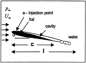
Figure 1: Ventilated foil parameters
With sufficient injection, a cavity is formed on the surface of the foil, leading to an increase in pressure on the suction side, resulting in a decrease in lift force. By varying the airflow rate, the cavity length and hence the resultant lift force can be adjusted.
There are several parameters influencing the ventilated flow problem. The geometrical parameters are shown in Figure 1. The angle of attack, α, is fixed for this problem and hence can be considered as a geometrical parameter. Operational parameters of importance include the ambient pressure and oncoming velocity, and the inlet air pressure and air velocity expressed together as the air flow rate Q. The dimensionless air flow rate per unit length is defined as (Lang et al. 1959):

(1)
The cavity pressure is given in terms of the ventilation number or the cavity number,
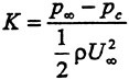
(2)
and is similar in definition to the cavitation number. However the relationship between K and CQ does not appear to be straightforward. Lang et al. (1959) noted that there appeared to be a relationship between the air flow rate and the cavity length and pressure that depended on the angle of attack. It was observed that beyond a certain CQ value nominally around 0.004, the
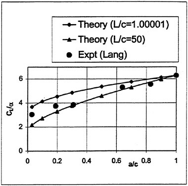
Figure 2: Lift coefficient derivative versus vent location
ventilation number was unaltered, and the increased airflow resulted in increased length of the cavity. A similar trend is noticeable from Fabula’s (1962) theory when cavity length is an order of magnitude larger than the chord length.
The three forces of importance for the foil are obviously the lift, drag and overturning moment However, for the purposes of this paper, we will concentrate primarily on the lift coefficient, with the proviso that drag penalties due to ventilation be left as future work within this project. The lift coefficient is given traditionally for two-dimensional sections as
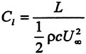
(3)
It is of interest to know the variation in lift coefficient with respect to the following two parameters:
-
vent location, given by the ratio a/c.
-
flow rate CQ, or the ventilation number K.
It is fairly obvious that maximum lift change will occur when the vent is located close to the leading edge, and this change will decrease as the vent moves leeward. The lift coefficient derivative should approach 2π as the vent approaches the trailing edge. These are indeed
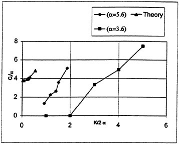
Figure 3: Lift coefficient derivative versus ventilation number/2α; experimental values of Lang et al. and theory of Fabula.
found to be the case, Figure 2, both from experimental results of Lang et al. (1959) and the theoretical results of Fabula (1962) using the closed cavity model. The open cavity model appeared to give unrealistic results for the case of cavity length slightly larger than 1, and for long cavity lengths, it gave results identical to the closed cavity model. So, only the closed cavity results are shown in Figure 2. The figure shows some interesting trends. The experiments closely agree with theory, even though the theoretical results pertain to a flat plate, while the experiments were conducted on a NACA 0010 foil. The figure indicates that unless thicker foils are used, results may not differ appreciably from the flat plate case. The foil case tends towards a value of π as the vent approaches the leading edge, indicating about 50% of lift can be dumped by ventilating the entire upper surface of a foil. It is interesting that much greater lift can be lost by using a flat plate, where the curve approaches a value of π/2, indicating a loss of 75% of the lift. It would be useful to evaluate how a thicker foil performs against these results.
Correlation of experimental and theoretical results for the case of a/c=0.3, and various Κ numbers are shown in Figure 3. There are undoubtedly few difficulties in precisely estimating the ventilation number in the experiments. While the trends between theory and experiment appear to be similar, albeit at different offsets, the experimental cases include data for partially vented conditions, while the theoretical curve is for the fully vented condition for different cavity lengths. Due to its limitations, the theory cannot be applied for partially vented conditions. Further, it is seen that much higher ventilation is required for the smaller angle of attack case (about 130% higher at Cl/α=4), which is not intuitively obvious. No clear conclusions may be drawn from this analysis. It is hoped that FLUENT simulations may show a clearer trend between Κ and Cl.
3. Numerical Simulation
Numerical simulations of ventilated foil flows are currently ongoing using FLUENT Ver 4.4, a pressure-based segregated finite-volume method solver. This software has a capability for solving multi-phase flows, with options for grid refinement around large pressure gradient locations. The simulations are expected to provide a means of obtaining fairly accurate results for ventilated foils that can be compared against corresponding results from experiments and theory.
The multi-phase model used in the simulations is the Volume Of Fluid (VOF) model included in FLUENT. In this model, a single set of momentum equations is used to describe both fluids, as given below:
(4)
where the density ρ, and dynamic viscosity μ are determined by tracking the volume fraction of each cell. The volume fraction (εk) of a cell is determined by solving the continuity equation for the fluids,
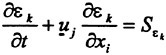
(5)
where Sεk denotes any source terms in the problem. A standard RNG k-ε turbulence model is used for closure. The momentum equations are solved using an explicit time stepping method, with a user-defined time step and maximum
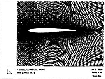
Figure 4: Computational grid in FLUENT
allowable iterations per time step. The volume fraction equation can be solved either at every iteration of the momentum equation, or for every time step. To speed up processing time, the latter option is used for the present simulations. Surface tension effects are included in the simulation, and the standard value of surface tension of water at 20° C is used.
The geometry and the mesh are created using a program called preBFC Ver. 3.0. The grid is a structured mesh with quadrilateral cells as required by FLUENT. The computational domain consists of 301 cells in the i direction and 151 cells in the j direction. The grid needs to be highly resolved near the foil for accurate modeling of the flow. Further, there is a requirement for significant resolution downstream to visualize the cavity, as the latter grows and moves downstream of the foil. This is accomplished with an O-H type grid, which consists of a cyclic boundary at the leading edge of the foil. A rectangular grid is used behind the foil to visualize the downstream cavity and any shed air bubbles. The O-grid at the foil surface is highly resolved, while aft of the foil, the Η-grid is coarser as x approaches xmax. The transition from circular to rectangular grid takes place half a chord length behind the foil. The two interior regions are each 100 cells by 101 cells giving a total of 45451 computational cells. The grid was smoothed using the “Spacing control” option in preBFC over the entire domain.
Results reported in this paper are obtained from simulations conducted on a NACA 0010 foil with 1 m chord length, and an air orifice width of 0.01 m. The flow conditions, similar to Lang et al. (1959), are as follows.
|
Air vent location |
3% chord |
|
Water inlet velocity |
10 m/s |
|
Air inlet velocity |
5 m/s |
|
Dimensionless air flow rate |
0.005 |
|
Ambient pressure |
1.3 E05 Pa |
Using a time step of 0.01 sec, the simulations were run up to t=1.9 sec. The simulation was started with the foil in the fully wetted condition, and air injection was initiated 0.3 sec into the simulation. It was observed that if air injection was started at t=0, the resulting air cavity showed a ballooning effect at the trailing edge due to the presence of the starting vortex, and this balloon was later swung around as the vortex moved downstream. The simulation results were unrealistic in this case. If the fully wetted flow was allowed to develop initially and then air injection introduced, the cavity was much better developed and simulation results were found to be reliable. With a total of 190 time steps and a maximum of 120 iterations per time step, the vented simulations took approximately 24 hours per case.
4. Results and discussion
The results presented and discussed in this section pertain to time evolution of the ventilated flow and foil characteristics for a NACA 0010 foil at zero angle of attack. A parametric study in terms of K and a/c are beyond the scope of this paper, but will be part of proposed research. Figures 5 a–d show the volume-averaged density contours as the flow develops over time. At t=0.54 sec (about 0.2 sec after air injection), the cavity shows signs of development, with the trailing wake showing a mixture of air and water. The cavity is well developed beyond 0.84 sec, and has extended downstream of trailing edge. With passage of time, the cavity continues to grow, albeit gradually, and the boundary layer comprising a mixture of water and air is evident all around the cavity. Patches of air-water mixture can also be seen in the trailing end of the cavity, which is due to entrainment of the slower flow into the cavity. The pressure contour plots (Figure 5 e–h) show that the trailing edge pressure point moves further
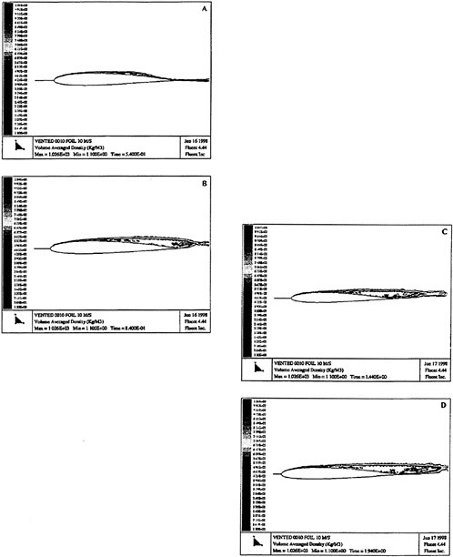
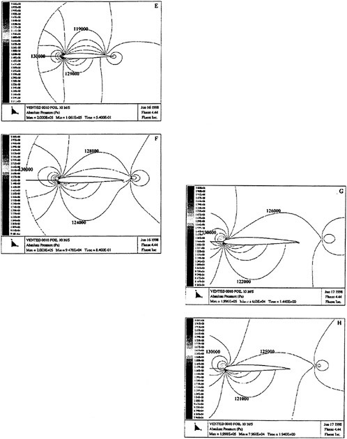
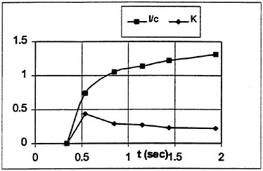
Figure 6: Variation of ventilation number (K) and cavity length (l/c) with time.
downstream as the cavity develops. The leading edge stagnation pressure values remain unaffected by the cavity development.
From the simulations, the cavity pressure and cavity length were estimated, and are plotted in Figure 6. The cavity number peaks initially, and then decreases gradually to level out at a value of about 0.22. The corresponding trend for the cavity length is a steep increase initially, and then a more gradual growth with time.
The cavity pressure and length can be expected to be interrelated. If at two instants of time, the cavity pressures and volumes are known, they can be related by the ideal gas law (assuming constant temperature):
(6)
The cavity volume depends on the net volume flow rate, i.e. the inflow from the vent minus the outflow through the boundary layer and the wake. The cavity length is proportional to the cavity volume, and the relationship may be assumed linear if perturbations in cavity thickness are small. Then, based on Eq. (6) the following relationship can be expected:
(7)
From the data in Figure 6, it is seen that this relationship is satisfied to within 10% over the time length specified, i.e.
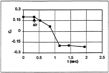
Figure 7: Change in lift coefficient with time for the NACA 0010 foil at zero angle of attack.
The ventilation number may thus be expected to vary as the inverse of cavity length during the primary stage of cavity development Experimental observations of Lang et al. (1959) showed unclear trends with respect to the ventilation number, but it was felt that K tends to remain a constant at later stages of the cavity development.
Figure 7 shows the change in lift coefficient with time for the NACA 0010 foil. The lift coefficient is originally at its fully wetted value of 0.2, gradually decreasing until the steady state cavity is developed at about 1.2 sec (0.9 sec after air injection). Cl is noticed to stabilize at around a value of −0.21±5%. This agrees well with Lang et al’s (1959) results where the least squared straight line fit to experimental Cl data intersects at −0.22 for zero angle attack. The data also shows that 90% of steady state lift value is achieved in less that 1 sec after air injection. This response time information is an important consideration when developing a ride control system. It is of interest to know how this time varies as the operational parameters are changed. This will be part of the future research in this project. This simulation has shown convincing evidence as to the utilization of FLUENT for simulation of the flow of interest.
5. Conclusion and future work
A reasonably comprehensive set of experimental data on lift coefficient for a NACA 0010 foil has shown good agreement with
theoretical results with respect to vent location, but unclear trends with respect to the ventilation number. Simulations conducted on the same foil with the commercial software FLUENT have shown good correlation with experimental data for the lift coefficient at zero degree angle of attack. The product of ventilation number and cavity length is found to be roughly a constant for the duration of cavity development.
Further work with FLUENT includes the following:
-
NACA 0010 foil at different angles of attack
-
Same foil with different vent locations.
-
Other foil sections of interest, and flow conditions of relevance to fast craft.
-
Studies on drag induced by ventilation.
-
Variations to the basic configuration of ventilated foils.
It is also proposed to use the leading-edge-corrected linear theory of Kinnas (1991) to compare with results of FLUENT.
The present work was initiated by the Australian fast ferry industry with a view to assess the feasibility and viability of using ventilated foils for ride control of high speed crafts. Ongoing simulations will provide farther information that would enable ventilated foils to be a proven alternative to incidence control as means of pitch control on a number of vessels, particularly fast ferries.
6. Acknowledgments
This work forms part of Australian Maritime Engineering CRC’s Program B: Performance of Surface Marine Vehicles. The work is supported by the industry participants of the research Task, Incat Designs Sydney through Mr. Todd Maybury, and Austal Ships through Mr. Tony Elms. The second author’s Masters work is supported by an Overseas Postgraduate Research Scholarship of the Australian Government, and an ΑΜΕ CRC Postgraduate Scholarship. The authors would like to acknowledge the help of Dr. Liang Cheng and Mr. Xiaojang Wang, Department of Civil Engineering, University of Western Australia for the use of their computer facilities and the FLUENT software for this project. Suggestions offered by Mr. Kim Klaka and Dr. Patrick Couser of ΑΜΕ Perth Research Core are appreciated.
7. References
Elms, Τ., “Hydrofoil Lift Control Using Air Injection” Bachelor of Engineering Thesis, University of New South Wales, 1992.
Fabula, Α., “Thin Air-foil Theory applied to Hydrofoils with a Finite Cavity and Arbitrary Free-Streamline Detachment” Fluid Mechanics, Vol. 12, Part 2, 1962
Fluent Inc, “Fluent User’s Guide Vol. 2” Fluent Inc, Lebenon, N.H, 1995.
Gunston, B., “Hydrofoils & Hovercraft, New Vehicles for Sea and Land”, New York, Doubleday, 1970.
Kinnas, S.A., “Leading-edge corrections to the linear theory of partially cavitating hydrofoils”, J. Ship Res. Vol. 35, No. 1, 1991, pp. 15–27.
Lang, T.G., “Base Vented Hydrofoils” NAVORD Report 6606, October 19, 1959.
Lang, T.G., Daybell, D.A., Smith, K.E. “Water-Tunnel Tests of Hydrofoils with Forced Ventilation”, NAVORD Report 7008, 10 November 1959.
Tulin, M. and Burkhart, M.P., “Linearized Theory for Flows About Lifting Foils at Zero Cavitation Number” Technical Report C-638, David Taylor Model Basin, Bethesda, MD, 1955.
Tulin, M., and Hsu, C.C., “New Applications of Cavity Flow Theory” Hydronautics, Inc Report, 1980.
Tulin, M., “Supercavitating Flow Past Foils and Struts” NPL Symposium on Cavitation in Hydrodynamics, Her Majesty’s Stationary Office, London, England, 1956.
DISCUSSION
T.Sarpkaya
Naval Postgraduate School, USA
If the physics of the desired control is to separate the boundary layer on the upper surface, why is the air introduction advantageous? Why not use water injection and avoid undesirable lift fluctuations? Even better, why not induce the boundary-layer separation point, and thereby control its angular motion (a few millimeters), the length of the separation zone, and thus the lift as in the case of thrust controls for missiles? Your comments will be appreciated.
AUTHORS’ REPLY
One of the reasons for using air introduction on the ride control foils is to overcome the force limitation cavitation puts on the foils. At the current speeds of high speed craft, most notably catamaran ferries, ride control foils are required to be quite large, thus heavy, to produce the required force without cavitating. Air injection on the surface of the foil gives the ability to greatly adjust the lift of the foil as well as delaying the onset of cavitation. While a movable plate along the foil would give us the ability to control the lift of the foil to a certain extent, it would invariably induce cavitation along the foil. Air injection allows greater control of the cavity along the entire foil with variable flow rates of injection and the ability to use multiple vents along the surface of the foil. By using a large flow rate injected at the leading edge, a large force can be generated to dampen motions in a heavy sea-state, whereas in relatively calm seas, short bursts can be initiated toward the trailing edge, thereby reducing drag when large damping forces are not needed.
The choice of air entrainment instead of using water is being pursued due to the ease of implementing such a system. While it is possible to use the surrounding water as the injection fluid, this would require a more robust support system than that of air injection. One of the aims of this project is to reduce the number of through-hulls below the waterline. Whereas atmospheric pressure can easily be supplied within the strut, water would require a port in the strut or along the hull. It was therefore decided that air would be a more advantageous medium.


