
Design System of Marine Propellers with New Blade Sections
C.Kawakita, T.Hoshino (Mitsubishi Heavy Industries, Ltd., Japan)
Abstract
This paper shows the design system of marine propellers with new blade sections based on the lifting-line method and lifting-surface method, i.e. QCM (Quasi-Continuous Method). In order to improve the cavitation performance, the new blade sections with the prescribed three-dimensional pressure distribution over blade surface are designed by the numerical optimization technique, i.e. SUMT (Sequential Unconstrained Minimization Technique) method. The propellers with new blade sections for a pure car carrier and a container ship were designed by this system. The open-water test and cavitation test of the designed propellers were carried out and compared with the conventional propellers with NACA series blade sections. It was found that the designed propellers with new blade sections had higher open-water efficiencies and better cavitation performances than those of the conventional propellers. The present system is a useful tool for designing the high performance marine propellers.
Nomenclature
|
a0 |
Leading edge radius |
|
C(r) |
Chord length |
|
CP(Pi) |
|
|
D |
Propeller diameter |
|
eP |
Efficiency of propeller |
|
f(X) |
Objective function |
|
F(X,rk) |
Modified objective function |
|
gic(X) |
Design constraint |
|
J |
Advance coefficient=VA/(nD) |
|
K |
Number of propeller blades |
|
KT |
Thrust coefficient of propeller =T/ρn2D4 |
|
KQ |
Torque coefficient of propeller =Q/ρn2D5 |
|
m |
Unit outward vector |
|
M |
Number of radial control points |
|
n |
Propeller rotational speed, [rps] |
|
n |
Unit vector normal to blade camber surface |
|
Ν |
Number of chordwise control points |
|
Nc |
The number of design constraints |
|
p0 |
Static pressure at infinity |
|
pν |
Vapor pressure |
|
p(Ρi) |
Pressure on blade |
|
Q |
Propeller torque |
|
r |
Radial coordinate from propeller axis |
|
rb |
Radius of propeller boss |
|
ri |
Radial coordinates of control point |
|
rk |
Perturbed parameter in SUMT method |
|
rμ |
Radial coordinates of loading point |
|
R |
Propeller radius |
|
s |
Chordwise coordinate for blade section |
|
t |
Unit vector tangent to blade camber surface |
|
T |
Propeller Thrust |
|
x,y,z |
Cartesian coordinates |
|
ν |
Velocity |
|
VA |
Speed of advance |
|
ν |
Induced velocity vector |
|
VG |
Induced velocity vector due to vortices |
|
VS |
Induced velocity vector due to sources |
|
Vl |
Velocity vector of relative inflow |
|
Wi |
Weighted coefficients |
|
X |
Design variable |
|
ΔΡij |
Difference between objective and calculated pressure at control point |
|
ΔCij |
Divided chord length |
|
θ |
Angular coordinate from generator line of propeller |
|
ρ |
Fluid density |
|
Ω |
Angular velocity |
|
σnc |
|
|
ξ |
Chordwise station at blade section |
|
ξc(ξ,r) |
Camber distribution |
|
ξt(ξ,r) |
Thickness distribution |
1. Introduction
Marine propellers with various blade geometry such as a highly skewed propeller are often fitted to ships in order to improve the cavitation performance, such as reducing the propeller-induced vibration and noise, or to improve the efficiency of the propeller. In the design of such propellers, the design charts based on methodical series tests are to be supplemented by the theoretical calculations of propeller open-water characteristics. The most familiar propeller design method, for given blade contour configuration and a selected blade section, is the use of lifting-surface theory [1,2]. The radial pitch and camber variations are determined by the lifting surface theory in order to match the given radial loading distribution and chordwise loading shape under the condition of circumferential averaged inflow velocity. In practical propeller design procedure which adopts the commonly used NACA66 thickness form and a=0.8 mean line [3], pitch and camber variation is determined such that the major loading comes from camber in a circumferential averaged inflow.
Recently, numerous researchers have adopted the Eppler’s theory [4] to design new blade sections by prescribing pressure distributions over the blade surface in order to improve the cavitation performance. Since Eppler and Shen [5,6,7] introduced Eppler’s design method of a subsonic wing sections into hydrofoil design, Eppler’s method has been widely accepted by the ship researchers and designers as a very good nonlinear and multi-points design method to explore new sections of hydrofoils and marine propellers. It is theoretically and experimentally verified that the cavitation buckets of the new sections are much wider than any other kind of sections such as NACA series.
The application of new blade sections onto propeller blades by Yamaguchi et. al. showed that the cavitation inception was delayed and fluctuating pressure and noise was reduced remarkably. In their first report [8], a propeller design procedure combining Eppler’s theory and the lifting surface theory were proposed and showed great effect of flat pressure distribution on reducing cavitation volume and fluctuating pressure. In their second report [9], the influences of designed lift coefficients of new blade sections on the reduction of fluctuating pressure and noise were investigated. The pressure distribution with higher pressure near the leading edge was more effective to increase the open-water efficiency and reduced the noise level. In their third report [10], the triangular pressure distribution with a negative peak at the leading edge was suggested to stabilize sheet cavitation and to suppress cloud cavity when its generation was possible.
Lee et al. [11] has suggested a different concept of propeller design procedure by developing a new blade section for a key radius of the propeller and using it onto all radii to avoid the difficulty of a different new section for each radius, and the difficulty of surface fairing and smoothing. Dang et al. [12] have developed a new and different propeller design procedure using new blade sections, which incorporates Eppler’s design code, the steady and unsteady lifting surface prediction codes and concept of equivalent 2-D sections.
Realization of the three-dimensional pressure distribution, even though it is known, is difficult as a matter of fact, since the Eppler’s theory treats only a two-dimensional foil section. In addition, blade surface fairing is needed after designing every section at each radius to form smooth blade geometry.
This paper shows the design system of marine propellers with new blade sections. The Quasi-Continuous Method (QCM) [2,17], one of the lifting surface theories, is applied to the numerical calculation of the propeller design. The new blade sections with the prescribed three dimensional pressure distributions over blade surface are designed by the numerical optimization technique, i.e. SUMT (Sequential Unconstrained Minimization Technique) method [23]. The new blade section is designed by specifying surface pressure distributions that minimize the cavitation phenomena. For example, surface pressure distributions are prescribed as minimizing the occurrence of local suction peaks at the section leading edge. It is possible to derive the blade sections, which have a superior cavitation performance to those based on the NACA series. Propeller efficiency would be increased by reducing the expanded area ratio while keeping the cavitation performance at the same level as that of the propeller with larger blade area by adapting the propeller with the new blade section which was designed by the present system.
The new propellers for a pure car carrier and a container ship were design by the present system. The model test results of the new propellers, such as open-water characteristics, cavitation patterns and fluctuating pressures induced on the hull, are presented.
2. Design Technique of Marine Propellers with New Blade Sections
The new propeller design procedure used in the
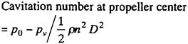
Nagasaki Experimental Tank, MHI. is shown in Fig. 1. Our new approach to propeller design incorporates five steps. Each step is repeated until the desired propeller performance is attained. We mention briefly each step as follows.
Step1: Design of standard propeller
The particulars of a propeller are determined from the data for resistance of the ship’s hull, self-propulsion factors, which indicate the interference between ship’s hull and the propeller, and model ship correlation factors, representing the scale effect of the hydrodynamic phenomena between model tests and full-scale operations. At this initial stage of the propeller design, propeller design charts obtained from systematic open-water tests of series propellers are used. Cavitation criteria, which gives the minimum expanded area from the viewpoint of cavitation performance of the propellers, and the beam theory to attain the strength of the propeller blades, are utilized.
Standard propellers are designed by using Mitsubishi-series (M-series) propeller design charts [13]. Even though Wageningen B-series [14]
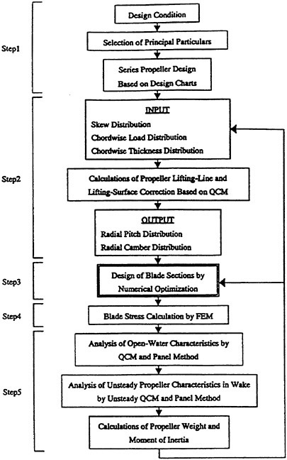
Fig. 1 Flow diagram of propeller design system
and MAU-series [15] propeller charts are widely known and used, MHI has developed its own M-series propeller charts and have been making efforts to expand the covering range and to improve their accuracy consistently. Fig. 2 shows the range of M-series propellers in view of the blade area ratio and pitch ratio. By using this chart, the principal dimensions, such as optimum propeller diameter, blade-expanded area and the number of propeller blades are easily decided.
Step2: Design of initial propeller with NACA blade section
The detailed geometry design follows, using existing propeller lifting-line and lifting-surface theories, to achieve the higher propeller efficiency and better cavitation performance.
The lifting-line calculation based on the Lerb’s lifting-line theory [16] is carried out for the circumferentially averaged ship wake distribution. The hydrodynamic pitch distribution, the induced velocities and the circulation distribution of an optimum wake adapted propeller or non-optimum wake adapted propeller are calculated. In the case of an optimum wake-adapted propeller, the problem is to determine the blade geometry for the distribution of the circulation to obtain the maximum value of the useful power for given quantities of power input, advance coefficient, and ship wake distribution.
The lifting-surface corrections to the results of the lifting-line calculation are calculated by QCM [2]. The blade shapes have the NACA a=0.8 camber lines and the modified NACA 66 thickness forms. This step is described in section 3 and 4.
Fig. 2 Range of M-series propellers
Step3: Design of new blade section
The NACA blade sections for the initial propeller are modified by the numerical optimization technique under the specifying surface pressure distributions for minimizing the cavitation phenomena. For example, the pressure distributions on the back-side of propeller are prescribed as flatter and higher at the section leading edge than those of NACA blade sections. It is possible to derive blade sections, which have a superior cavitation performance to those based on the NACA series. This step is described specifically in section 5. If the performance of the initial propeller is enough to the design purpose, this step is able to skip.
Step4: Evaluation of blade strength
The blade strength is checked in accordance with the rules of ship classification societies. Then the static stress distribution on the blade surface is analyzed by using Finite Element Method(FEM). The dynamic blade stress is examined by a system in which unsteady QCM(UQCM) [18] and FEM are combined. In addition, MHI has been accumulating the data of dynamic stress of the propeller blade in transient ship operation mode by model tests.
Step5: Estimation of hydrodynamic performance
Finally, the propeller open-water characteristics are calculated by the QCM and panel method [19,20]. The unsteady characteristics of the propeller in wake are estimated by the UQCM and unsteady panel method [21].
In propeller design, not only evaluation of propeller open-water characteristics but also evaluation of cavitaion erosion and excitation forces due to cavitating propellers become most important items to be considered. Needless to say, since the cavitation phenomena on the propeller blades are not yet established. Thus, the cavitation performance is usually evaluated by the simple calculation method based on UQCM. In this method, the cavity range on the blade surface is estimated by using the empirical method of equivalent lift, and cavity thickness by open-type cavity models [22].
A performance of the designed propeller is confirmed by the experiments in a towing tank and in a cavitation tunnel with the propeller model, which is precisely manufactured by a 5-axis numerically controlled milling machine.
3. Numerical Solution of Lifting-Surface Problems based on QCM
A Quasi-Continuous Method (QCM) was developed by Lan [23] to improve the conventional Vortex Lattice Method (VLM) through the theoretical considerations so that the wing edge and Cauchy singularities may be properly accounted for. The QCM has both advantages of the Mode Function Method (MFM) and the VLM; the load distribution is assumed to be continuous in the chordwise direction and stepwise constant in the spanwise direction. Simplicity and flexibility of the VLM are also retained. Therefore, the complex blade geometries involving the high skew and extreme changes in pitch of a propeller can be taken into consideration correctly. The QCM was firstly applied to steady propeller problems [17] and extended to the unsteady propeller problems [18].
3.1. Coordinate Systems
Let us consider now a propeller rotating clockwise with a constant angular velocity Ω in an inviscid and incompressible flow with a uniform velocity VA far upstream. The propeller consists of Κ blades of identical shape axisymmetrically attached to a boss. In representing the geometrical shape of the propeller, we define a Cartesian coordinate system O-xyz fixed on the propeller as shown in Fig. 3. The z-axis coincides with the generating line of the first blade.
A cylindrical coordinate system is defined as follows. Angular coordinate θ is measured clockwise from the z-axis when viewed in the direction of positive x. Radial and angular coordinates are given by
(1)
Then, the Cartesian coordinate system O-xyz is transformed into the cylindrical coordinate system O-xr θ by the relation
(2)
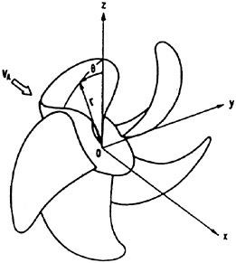
Fig. 3 Coordinate systems of propeller
3.2. Numerical Modeling of Propeller and Trailing Vortex Wake
Propeller blades are represented by the distributions of vortices and sources on the mean camber surfaces of the blades together with the associated distribution of vortices shed into the wake. The vortex system, i.e. the distribution of horseshoe vortices which consist of bound vortices and free vortices shed from both edges of bound vortices, represents blade loading and wake, and the source distribution represents blade thickness.
Continuous distributions of bound vortices and sources are replaced with quasi-continuous ones according to QCM. Thus, the blade surfaces are covered with a number of vortex and source strips.
In selecting the radial loading stations, it should be noted that the better results could be obtained if the finer strips are used in the region of rapid variation of the sectional properties. The well-known semicircle method is suitable for this purpose. The radial interval from the boss r=rb to the tip r=R is divided into a suitable number of M strips. The loading stations rμ (radial coordinates of loading points) and the control stations ri (radial coordinates of control points) of the strips are defined as
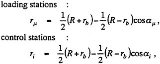
(3)
where
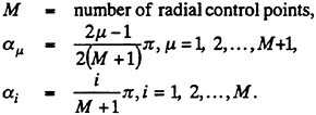
According to the QCM, the chordwise loading points and the control points at each radius are arranged as follows:
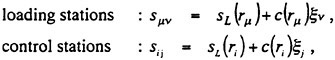
(4)
where
sL(r)=chordwise coordinate of leading edge,
c(r)=chord length of blade section,
Ν=number of chordwise control points,
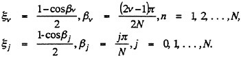
The arrangement of the loading points and the control points selected for the present method is illustrated in Fig. 4.
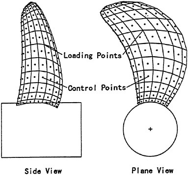
Fig. 4 Arrangement of loading point and control point
The free vortices shed from the bound vortices on the mean camber surfaces are considered to leave the trailing edge of the blade and flow into the slipstream with the local velocity at that position. Usual approach is to approximate the trailing vortex sheet by a prescribed helical surface, in order to avoid the time consuming calculation of the slipstream velocities. In the present method, the roll-up of the slipstream is not accounted for. The trailing vortices are extensions of the chordwise vortices on the blade and leave the trailing edge in the direction tangent to the mean camber surface so as to satisfy the Kutta condition. After that the pitch of the trailing vortices changes linearly with respect to the angular coordinate and reaches an ultimate value. In the downstream, the trailing vortices become the helical lines with the ultimate constant pitch. Then, the trailing vortex sheet consists of M+1 concentrated trailing vortex lines whose trailing edge coordinate match the corresponding values of the vortex strips on the blades.
3.3. Calculation of Induced Velocities
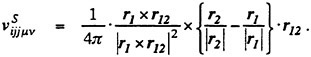
The induced velocity at a control point Pij due to a line vortex segment of the unit strength (see in Fig. 5) can be expressed by the Biot-Savart’s law as
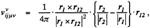
(5)
where
r12=r2−r1.
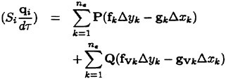
Here we consider a horseshoe vortex of unit strength, which consists of a bound vortex placed at Qμν and Qμ+1ν and two free vortices shed from Qμν and Qμ+1ν in the chordwise direction along loading stations as shown in Fig. 5. The induced velocity ![]() at a control point Pij due to this horseshoe vortex is calculated by
at a control point Pij due to this horseshoe vortex is calculated by
(6)
where the superscripts B, F and W express the induced velocities due to the bound and free vortices and the trailing vortices, respectively.
Let the strength of bound vortex on the μ-th vortex strip be γμ(s). Then the induced velocity  at Pij due to the closed vortices on the vortex strip and in the wake is expressed by using a characteristic of the QCM as
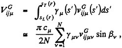
(7)
where
The induced velocity at a control point Pij due to the whole vortex systems is given by the following equation
(8)
where the suffix k shows the contribution from the k-th blade.
Next, let us consider the induced velocity due to the source distribution. The induced velocity at a control point Pij due to a source segment of unit strength is given in a manner similar to that of the vortex segments by
(9)
Denoting the strength of the source by σμν, the induced velocity at the control point Pij on the blade due to the whole source distribution is expressed as
(10)
The total fluid velocity at each control point Pij can be written as a sum of the contributions of the singularity distributions together with the total relative inflow:
(11)
where
i=1, 2,…, M, j=1, 2,…, Ν, k=1, 2,…, Κ,
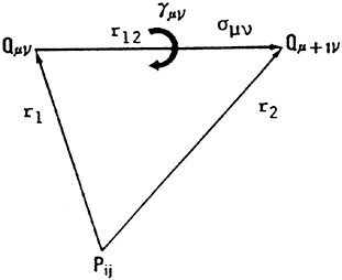
Fig. 5 Vortex and source segments
4. Numerical Method for Initial Propeller Design
4.1. Determination of Vortex and Source Distributions
The radial circulation distribution can be obtained from a lifting-line theory such as the Lerbs’ induction factor method [16] for the circumferentially averaged inflow. The strength of each vortex element is then obtained by distributing the total bound circulation over the chord. The NACA a=0.8 distribution is usually used for the chordwise load distribution.
As for the chordwise thickness form, the NACA 16 thickness form or the DTNSRDC modified NACA 66 thickness form is frequently used for propellers. The strength of each source element can be determined by the product of chordwise derivative of the blade thickness and the relative inflow velocity.
4.2. Calculation of Blade Geometry
The components of the inflow velocity can be expressed in the Cartesian coordinate system as
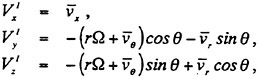
(12)
where ![]() are the cylindrical components of the circumferentially averaged inflow velocity. Then the total fluid velocities at control points are obtained from Eq. (11). The normal and tangential components of the total velocity to the mean camber surface are then obtained as
are the cylindrical components of the circumferentially averaged inflow velocity. Then the total fluid velocities at control points are obtained from Eq. (11). The normal and tangential components of the total velocity to the mean camber surface are then obtained as
(13)
where
nij=unit normal vector at the control point to mean camber surface,
tij=unit tangent vector at the control point to mean camber surface.
The unit normal vector nij is obtained from the cross product of the two diagonal vectors connecting the opposite corners of each quadrilateral element composed of the four loading points surrounding a control point and its positive direction is taken from face to back side. The unit tangent vector tij is obtained from the average of the two chordwise vectors of each quadrilateral element and its positive direction is taken from the leading edge to the trailing edge.
Following Greeley and Kerwin [1], the incremental slope of the mean camber surface are expressed as
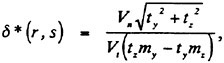
(14)
where
ty, tz=y- and z-components of unit tangent vector tij, respectively,
my, mz=y- and z-components of unit outward vector mij, respectively.
The unit outward vector mij can be obtained as
(15)
If the incremental slope δ*(r, s) is evaluated at all control points, the new mean camber line can be obtained by integrating the slope from the leading edge to the point considered as
(16)
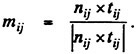
The integrated value δ(r, s) is usually divided into the pitch angle correction Δβ(r) and the camber correction Δf(r, s), which are expressed as
(17)
where sT(r) is the chordwise coordinate of the trailing edge of the blade.
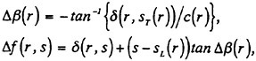
If the pitch angle correction and the camber correction are obtained, a new blade surface is formed by correcting the original pitch angle β0(r) and the original camber line f0(r, s) as
(18)
Then, the new blade surface can be used as the surface on which the source and vortex are to be distributed in the next step. This process is repeated until the correction to the blade surface is sufficiently small.
In the present paper, the iteration starts with a trial surface having a pitch distribution corresponding to the hydrodynamic pitch angle βi(r) from the lifting-line theory and a zero camber line. After three iterations, the corrections Δβ(r) and Δf(r, s) become almost zero because of high convergence of the present method. Therefore, the blade surface obtained after three iterations may be considered to be the final one.
5. Design of Blade Sections by Numerical Optimization
5.1. Optimization Problem and Nonlinear Programming
The technique, which solves various optimization problems (minimizing or maximizing) by mathematical method, is called the optimization method or the mathematical programming. The optimization method is one of the most powerful methods in the optimization method. We mention briefly the important terms and definitions for optimization problems.
Design Variable: The design variables are expressed the object of design, when these variables are given, the design is decided. In the propeller design, it is considered that the design variables are principal dimensions and approximation coefficients that represent the propeller shape. In this paper, a set of variables is written by vector form as X.
Design Constraint: The design constraints are considered the equality and inequality forms that are represented the physical or practical limitations. A function of the design variables are given as follows,
gic(X)≧0 (ic=1, 2,…., Nc).
Objective Function: The objective function represents the object of optimizing in the problem. In the propeller design, we consider the function that the propeller efficiency or the pressure distribution on the blade is evaluated. A function of the design variables is given as f(X).
The definition of the optimization problem is obtaining the design variables X that minimize the objective functions f(X) under the design constraints gic(X)≧0 (ic=1, 2,…., Nc). A nonlinear programming usually solves the nonlinear programming problem that includes a nonlinear function in either the objective functions or the constraints.
The nonlinear programming in this paper consists of three stages.
-
Process of constraint
We use the SUMT (Sequential Unconstrained Minimization Technique) method [24] that is one of the penalty function method. The SUMT method changes the constrained optimization problem for the unconstrained optimization problem formally by adding some functions that include the effect of design constraints to the objective function.
-
Minimum value search method for function of several variables
After processing of constraint, we use the Zangwill method [25] for a minimum value direct search method. The Zangwill method is able to search stable in order to have no use for the derivative.
-
Line search method
The search method is usually iterative method that consists of repetition by a line search method. This paper uses a quadratic interpolation method without using the derivative.
The problem, which applies the nonlinear programming to the propeller design, accompanies with several complicated objective functions and constraints. It is considered that the direct search method is stable for optimization in order to have no use for the derivative and can get the good results for deciding the shape at any calculation time.
5.2. SUMT Method
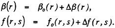
We describe the SUMT method that is used for optimization in this paper briefly. The SUMT method called the interior point method is one of the penalty function method that changes the constrained optimization problem for the unconstrained optimization problem formally by adding some functions (penalty term) that include the effect of design constraints to the objective function. The optimization problem usually uses the following transformation as,
(19)
This transformation is called the SUMT transformation. We called that rk is the perturbed parameter and F(X,rk) is the modified objective function. Applying the SUMT method, the optimization problem is written as follows,
“Obtaining the design variables X that minimize the objective function f(X) without the design constraints, however, rk decreases gradually by k times minimization.”
The nonlinear programming that minimized the modified objective function with SUMT transformation by the Zangwill direct search method is simply called the SUMT method in this paper.
5.3. Propeller Design by SUMT Method
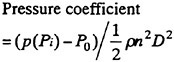
The new blade sections with the three-dimensional prescribed pressure distribution over blade surface are designed by using the SUMT method. The blade optimization starts from NACA blade sections of the initial propeller. The main purpose of the new blade sections is to improve the cavitation performance, such as fluctuating pressure or cavitation erosion, than NACA blade sections. The pressure distribution (objective pressure distribution) on the back-side of the propeller blade is especially important for the cavitation performance, given as the pressure coefficients ![]() . In order to keep the same sectional blade lift coefficients Cl(r), the pressure coefficients on the face-side of the blade
. In order to keep the same sectional blade lift coefficients Cl(r), the pressure coefficients on the face-side of the blade ![]() are decided automatically as
are decided automatically as
(20)
where
![]() =pressure coefficients on the back-side of the initial blade sections,
=pressure coefficients on the back-side of the initial blade sections,
![]() =pressure coefficients on the face-side of the initial blade sections.
=pressure coefficients on the face-side of the initial blade sections.
In this operation, the thrust coefficient KT at design point for the optimized propeller can be kept the same level as the initial propeller.
The pressure distributions are prescribed at the several representative radial positions (at the control point radius). The each blade section is modified to satisfy the pressure distribution given at the design condition by the SUMT method. The pressure coefficient distributions on the propeller blade, ![]() and
and ![]() are calculated by QCM in a circumferential averaged ship wake.
are calculated by QCM in a circumferential averaged ship wake.
The objective function f(X) is defined as,
(21)
where
ΔCPij: 
ΔCij: divided chord length,
Wi: weighted coefficients.
The role of the weighted coefficients takes precedence of optimizing blade section near propeller tip at which occurred the cavitation easily. The pressure distribution on the new blade section is close to the objective pressure distribution by minimizing the objective function.
The blade sections at each radial position r can be expressed by the superposition of the thickness and camber distributions in the chordwise direction. Expressing the thickness distribution as ξt(ξ,r) and the camber distribution as ξc(ξ,r), the back-side surface (ξΒ,ηB) and the face-side surface (ξF,ηF) of the blade section are written as,
(22)
where
θc=tan−1(dηc/dξ)
Since a coordinate system normalized by the each chord length C(r) of the propeller blade is used in this expression, a range of ξ should be given as,
0≤ξ≤1.
The thickness and camber distributions ξt(ξ,r), ξc(ξ,r) are approximated by the polynomial expressions which are used six kinds of functions in the radial direction as follows,
ξcmax(r)=maximum camber point in the chordwise direction,
θc(0,r)=θc at the leading edge,
θc(1,r)=θc at the trailing edge,
ξtmax(r)=maximum thickness point in the chordwise direction,
θc(1,r)=tan−1(dηt/dξ) at the trailing edge,
a0(r)=leading edge radius.
These functions in the radial direction are given by 4th or 5th order polynomial. In this paper the polynomial coefficients of these functions are defined as the design variables. The radial distributions of pitch, maximum camber, maximum thickness, skew and rake are kept same as the distributions of the initial propeller.
In propeller blade design problem by means of the SUMT method, a set of suitable design constraints can be introduced to get the practical design and available results. In the present problems, the suitable constraints should be introduced in order to get reasonable blade sections. The constraints are given as follows,
(23)
The system of designing the blade sections by the SUMT method consists of 4 parts as follows.
Part 1: Initial set up
The NACA blade sections are approximated by the polynomial expressions. The initial propeller with NACA series blade sections is calculated by QCM at design point.
Part 2: Set up the objective pressure distribution
The objective pressure distributions on the blade sections at the several radial positions are given by the polynomial coefficients. The propeller designer decides the prescribed pressure distribution in order to improve the cavitation performance by comparing with NACA blade section.
Part 3: Optimization for blade section by SUMT
The polynomial coefficients which represent the
blade section, such as ξtmax(r) and ξcmax(r), set the design variables. They are optimized by the SUMT method as minimizing the objective function.
Part 4: Check the optimized blade sections
The optimized blade sections are checked whether enough or not, by comparing between the optimized pressure distribution and the objective pressure distribution. If the optimization process is not enough, the objective pressure distribution is changed a little. The optimization process is tried again from STEP3.
In order to check the effect of this system, three kinds of typical pressure distributions, (a) triangular pressure distribution, (b) semi-flat pressure distribution, (c) flat pressure distribution with higher pressure at leading edge were given on the back-side of a propeller. The final results (optimum) of the pressure distributions and blades are shown in Fig. 6 respectively, comparing with the initial and objective pressure distributions, and the initial NACA66 a=0.8 blade section. The optimized pressure distributions are almost close to the objective pressure distributions. It is considered that this optimization system is enough for the practical use. Small errors are shown in each case. In this optimization system, the fairness of the blade section in the chordwise and radial direction is prior to the optimization by using some functions for expressing the propeller shape. The fairness is important from the hydrodynamic and blade-strength point of view. It is considered that giving a priority to the fairness causes these small errors.
The optimized blade sections for triangular and semi-flat pressure distributions have thin thickness near the trailing edge as shown in Fig 6 (a) and (b). The early pressure recovery on the back-side of blade section tends to be thin thickness near the trailing edge by using the present system.
6. Numerical Examples
In order to evaluate the applicability of the present system, the propellers with new blades sections were designed for a pure car carrier and a container ship. The model tests of the designed propellers, such as the propeller open-water test and the cavitation test, were carried out in the towing tank and in the cavitation tunnel at Nagasaki Experimental Tank, MHI. The cavitation test, cavitation observation and fluctuation pressure measurement, were carried out in the wake field simulated by a wire mesh screen. The fluctuating pressure was measured on a flat plate above a propeller.
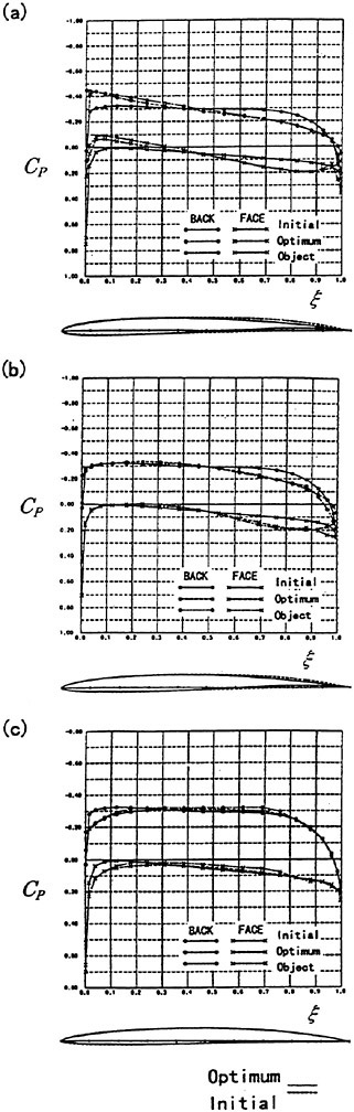
Fig. 6 Comparison of pressure distributions and blade sections at radial position 0.7R
(a) Triangular pressure distribution
(b) Semi-flat pressure distribution
(c) Flat pressure with higher pressure at leading edge
6.1. Propellers for a Pure Car Carrier
In the first example, we designed new propellers for a pure car carrier (PCC) by the present design system. Main particulars of the PCC are shown in Table 1. Two kinds of propellers (PCC2, PCC2S) were designed for evaluating the new blade sections based on the initial propellers (PCC1, PCC1S). PCC1 and PCC2 are conventional propellers, PCC1S and PCC2S are highly skewed propellers. PCC1 with MAU blade section and PCC1S with NACA66 a=0.8 blade section were initial propellers. PCC2 and PCC2S have new blade sections designed for aiming at low-pressure fluctuations and high efficiency by the present system based on the initial propellers. The design point was selected as ![]() . The principal particulars of the designed propellers are shown in Table 2 together with the initial propellers. The full-scale axial wake distribution estimated from the model test result is shown in Fig 7. The pressure distributions at 0.69R of the designed propeller calculated by QCM in a circumferential averaged wake are shown in Fig. 8. The pressure distributions on the back-side of new blade sections were prescribed as the flat with high pressure at the leading edge.
. The principal particulars of the designed propellers are shown in Table 2 together with the initial propellers. The full-scale axial wake distribution estimated from the model test result is shown in Fig 7. The pressure distributions at 0.69R of the designed propeller calculated by QCM in a circumferential averaged wake are shown in Fig. 8. The pressure distributions on the back-side of new blade sections were prescribed as the flat with high pressure at the leading edge.
Table 1 Principal particulars of PCC
|
Length between perpendiculars |
170.0 m |
|
Breadth |
32.2 m |
|
Draft |
8.5 m |
|
Power of engine (BHP) |
14500 PS |
|
Propeller revolution |
110 rpm |
Table 2 Principal particulars of designed propeller for PCC
|
|
PCC1 |
PCC2 |
PCC1S |
PCC2S |
|
Diameter |
6.1 |
|||
|
Pitch ratio |
0.889 |
0.891 |
0.971 |
0.962 |
|
Expanded area ratio |
0.554 |
0.449 |
||
|
Boss ratio |
0.1656 |
|||
|
Blade Section |
MAU |
NEW |
NACA |
NEW |
|
Rake angle |
0.0° |
−3.0° |
||
|
Skew angle |
13.8° |
25.9° |
||
|
Number of blade |
5 |
|||
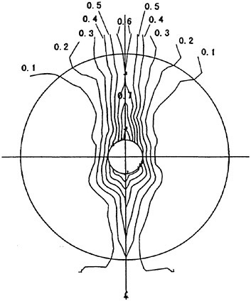
Fig. 7 Simulated wake distribution of PCC at the propeller plane
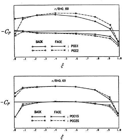
Fig. 8 Comparison of calculated pressure distributions for designed propellers at radial position 0.69R
The panel arrangements for PCC2 and PCC2S used in the panel method are shown in Fig. 9 and Fig. 10. An example of the accuracy for calculation results of the open-water characteristics of PCC2S by using QCM and panel method is shown in Fig. 11, comparing with experiments. The calculated results of QCM and panel method are in good agreement with experimental results. It is considered that QCM and the panel method can evaluate the open-water characteristics for the new propeller.
Efficiencies resulted in the open-water test are compared among the four designed propellers as shown in Fig. 12. Open-water efficiency of PCC2 is same as that of PCC1. Open-water efficiency of PCC2S is highest of the four, and 0.6% higher than that of PCC2, and 1.5% higher than that of PCC1 due to reducing the blade area.
The sketches of the observed cavitation patterns for all propellers under the test condition fixed as ![]() and σnc=2.1 are shown in Fig. 13.
and σnc=2.1 are shown in Fig. 13.
Fig. 9 Panel arrangement for PCC2 used in the panel method
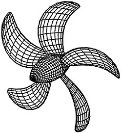
Fig. 10 Panel arrangement for PCC2S used in the panel method
The cavity extents of PCC2 and PCC2S with new blade sections are smaller than those of other propellers with MAU and NACA66 a=0.8 blade sections. The cavity of PCC2 is observed unstable.
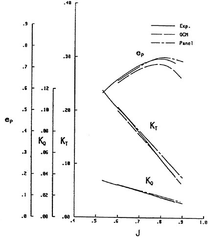
Fig. 11 Open-water characteristics for experiment and calculations of PCC2S
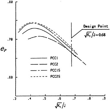
Fig. 12 Comparison of efficiencies for designed propellers of PCC, based on open-water model test results
Comparison of the pressure fluctuations of 1st blade frequency at center position above the propeller is shown in Fig. 14. The pressure fluctuation level of PCC2 of 1st blade frequency is reduced by about 45% compared to those of PCC1. The pressure fluctuation level of PCC2S is lower compared to those of other propeller. The pressure fluctuation level of PCC2S of 1st blade frequency is reduced by about 50% compared to those of PCC1 in spite of reducing the blade area, and reduced by about 5% compared to those of PCC2.
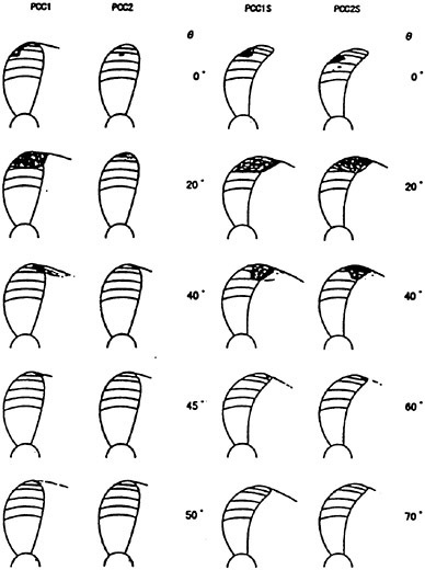
Fig. 13 Comparison of observed cavitation patterns for designed propellers of PCC
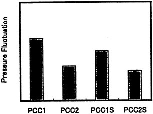
Fig. 14 Comparison of pressure fluctuations of 1st blade frequency above propeller center for designed propellers of PCC, based on cavitation test results
According to these results, the overall performance of the PCC2S in terms of efficiency, cavitation behavior and fluctuating pressure, is the best among the four propellers. It is considered that the effect of the designed new blade section is to improve the cavitation performance.
6.2. Propellers for a Container Ship
As the next example, we designed new propellers for a container ship by the present design system. Main particulars of the container ship are shown in Table 3. Three kinds of propellers (CS2, CS3, CS4) were designed for evaluating the new blade sections based on the initial propeller (CS1) with NACA66 a=0.8 blade section. CS2, CS3 and CS4 have new blade sections designed for aiming at low-pressure fluctuations and high efficiency by the present system. The design point was selected as ![]() . The principal particulars of four propellers are shown in Table 4. The full-scale axial wake distribution estimated from the model test result is shown in Fig 15.
. The principal particulars of four propellers are shown in Table 4. The full-scale axial wake distribution estimated from the model test result is shown in Fig 15.
Table 3 Principal particulars of Container Ship
|
Length between perpendiculars |
260.0 m |
|
Breadth |
39.7 m |
|
Draft |
11.0 m |
|
Power of engine (BHP) |
57000 PS |
|
Propeller revolution |
90 rpm |
Table 4 Principal particulars of designed propeller for Container Ship
|
|
CS1 |
CS2 |
CS3 |
CS4 |
|
Diameter |
8.5 |
|||
|
Pitch ratio |
1.12 |
1.10 |
1.09 |
1.11 |
|
Expanded area ratio |
0.740 |
|||
|
Boss ratio |
0.2024 |
|||
|
Blade Section |
NACA |
NEW |
NEW |
NEW |
|
Rake angle |
−3.0° |
|||
|
Skew angle |
25° |
|||
|
Number of blade |
6 |
|||
The pressure distributions at 0.7R of the designed propeller calculated by QCM in a circumferential averaged wake are shown in Fig. 16. The prescribed pressure distributions on the back-side of new blade sections for CS3 and CS4 were given the flat with high pressure at the leading edge, same as the design thought of the case for PCC. The pressure distributions for CS2 were prescribed as the flat pressure distribution with slightly decreasing near the leading edge.
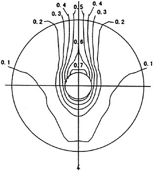
Fig. 15 Simulated wake distribution of Container Ship at the propeller plane
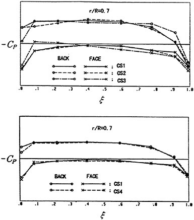
Fig. 16 Comparison of calculated pressure distributions for designed propellers at radial position 0.7R
The panel arrangement for CS4 used in the panel method is shown in Fig. 17. Calculated results of the open-water characteristics of CS4 by using QCM and panel method are shown in Fig. 18, comparing with experiments. The calculated results of QCM and panel method are in good agreement with experimental results, same as the case of PCC.
Efficiencies resulted in the open-water test are compared among the four designed propellers as shown in Fig. 19. Open-water efficiency of CS2 is highest of the four, and 0.2% higher than that of CS1. Open-water efficiency of CS3 is 1.0% lower than that of CS1. Open-water efficiency of CS4 is same as that of CS1.
Fig. 17 Panel arrangement for CS4 used in the panel method
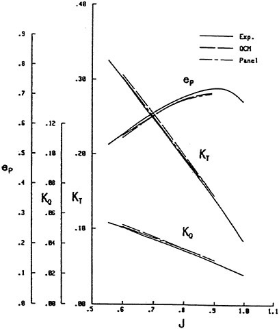
Fig. 18 Open-water characteristics for experiment and calculations of CS4
The sketches of the observed cavitation patterns for all propellers under the test condition fixed as ![]() and σnc=1.8 are shown in Fig. 20. The cavity extents of CS3 are smaller than those of other propellers. The cavity of CS3 and CS4 are observed unstable.
and σnc=1.8 are shown in Fig. 20. The cavity extents of CS3 are smaller than those of other propellers. The cavity of CS3 and CS4 are observed unstable.
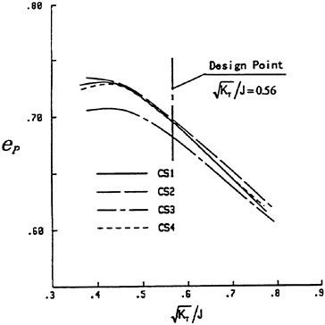
Fig. 19 Comparison of efficiencies for designed propellers of the container ship, based on open-water model test results
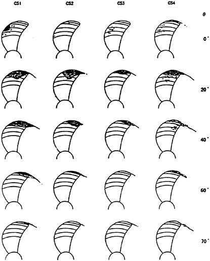
Fig. 20 Comparison of observed cavitation patterns for designed propellers of the container ship
Comparison of the pressure fluctuations of 1st blade frequency at center position above the propeller is shown in Fig. 21. The pressure fluctuation level of CS2 of 1st blade frequency is increased by about 70% compared to those of CS1. The pressure fluctuation level of CS3 and CS4 of 1st blade frequency are reduced by about 60% and 30% respectively compared to those of CS1.
According to these results, the overall performance of the CS4 in terms of cavitation behavior and fluctuating pressure, is the best among the four propellers.
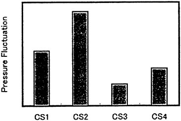
Fig. 21 Comparison of pressure fluctuations of 1st blade frequency above propeller center for designed propellers of the container ship, based on cavitation test results
7. Concluding Remarks
In this paper, the design system of marine propellers with new blade sections based on the lifting-line method, Quasi-Continuous Method (QCM) and Sequential Unconstrained Minimization Technique (SUMT) was presented. In order to improve the cavitation performance as compared with the propeller with NACA series blade section, the new blade sections with the prescribed three-dimensional pressure distribution over blade surface are designed by the present system. In order to evaluate the applicability of the present design system, the propellers with new blade sections for a pure car carrier and a container ship were designed. The open-water test and cavitation test of the designed propellers were carried out and compared with the conventional propellers with NACA series blade sections. It was found that the designed propellers with new blade sections had higher open-water efficiencies and better cavitation performances than those of the conventional propellers. The present system is a useful tool for designing the high performance marine propellers.
Acknowledgments
The authors would like to acknowledge the cooperation of stuff of the Nagasaki Experimental Tank of the Nagasaki Research and Development Center, Mitsubishi Heavy Industries, Ltd.
References
[1] Greelely, D.S. and Kerwin, J.E., “Numerical Methods for Propeller Design and Analysis in Steady Flow,” Trans. SNAME, Vol. 90. 1982, pp. 415–453.
[2] Hoshino, T. and Nakamura, N., “Propeller Design and Analysis Based on Numerical Lifting-Surface Calculations,” CADMO 88, Southampton, Sept. 1988, pp. 549–574.
[3] Abbott, I.H. and Von Doenhoff, A.E., Theory of Wing Sections, Dover Publications.
[4] Eppler, R. and Somers, D.M., “A Computer Program for the Design and Analysis of Low-Speed Airfoils,” NASA Technical Memorandum 80210, 1980.
[5] Eppler, R. and Shen, Y.T., “Wing Sections for Hydrofoils—Part 1: Symmetrical Profiles,” Journal of Ship Research, Vol. 23, No. 3, Sept. 1979, pp. 209–217.
[6] Shen, Y.T. and Eppler, R., “Wing Sections for Hydrofoils—Part 2: Nonsymmetrical Profiles,” Journal of Ship Research, Vol. 25, No. 3, Sept. 1981, pp. 191–200.
[7] Shen, Y.T., “Wing Sections for Hydrofoils—Part 3: Experimental Verifications,” Journal of Ship Research, Vol. 29, No. 1, March 1985, pp. 39–50.
[8] Yamaguchi, H., Kato, H., Tokano, S. and Maeda, M., “Development of Marine Propellers with Better Cavitation Performance (1st Report: Propellers with less cavitation),” Journal of The Society of Naval Architects of Japan, Vol. 158, Nov. 1985, pp. 69–80.
[9] Yamaguchi, H., Kato, H., Kamijo, A. and Maeda, M., “Development of Marine Propellers with Better Cavitation Performance (2nd Report: Effect of design lift coefficient for propellers with flat pressure distribution),” Journal of The Society of Naval Architects of Japan, Vol. 163, May 1988, pp. 48–65.
[10] Yamaguchi, H., Kato, H., Sugatani, A., Kamijo, A., Honda, T. and Maeda, M., “Development of Marine Propellers with Better Cavitation Performance (3rd Report: Pressure distribution to stabilize cavitation),” Journal of The Society of Naval Architects of Japan, Vol. 164, Nov. 1988, pp. 28–42.
[11] Lee, J.T., Kim, M.C., Ahn, J.W. Kim, K.S. and Kim, H.C., “Development of Marine Propellers with New Blade Sections for Container Ships,” Proceedings of Propellers Shafting 91 Symposium, Virginia Beach, Virginia, 1991.
[12] Dang, J, Chen, J. and Tang, D., “A Design Method of Highly Skewed Propellers with New Blade Sections in Circumferentially Non-uniform Ship Wake,” China Sip Scientific Research Center Report English version 92004, 1992.
[13] Taniguchi, K., “Study on Propeller Open-Water Characteristics”, Trans. of The West Japan Society of Naval Architects,” Vol. 3, 1951, Vol. 4, 1952.
[14] van Lammeren, W.P.A. et al., “The Wageningen B-screw Series,” Trans. SNAME, Vol. 77, 1969.
[15] Yazaki, A. et al., “Open-Water Test Series with Modern Five-, Six- Modified AU-Type Four Blades Propeller,” Journal of The Society of Naval Architects of Japan, Vol. 102, 1958, Vol. 106, 1960, Vol. 108, 1960, Vol. 125, 1965 and Vol. 131, 1972.
[16] Lerbs, H.W., “Moderately Loaded Propellers with a Finite Number of Blades and a Arbitrary Distribution of Circulation,” Trans. SNAME, Vol. 60, 1952, pp. -73–123.
[17] Nakamura, N., “Estimation of Propeller Open-Water Characteristics Based on Quasi-Continuous Method,” Journal of the Society of Naval Architects of Japan, Vol. 157, May 1985, pp. 99–111.
[18] Hoshino, T., “Application of Quasi-Continuous Method to Unsteady Propeller Lifting-Surface Problems,” Journal of the Society of Naval Architects of Japan, Vol. 158, Dec. 1985, pp. 51–71.
[19] Hoshino, T., “Numerical and Experimental Analysis of Propeller Wake by Using a Surface Panel Method and a 3-Component LDV,” 18th Symposium on Naval Hydrodynamics, 1990, pp. 297–317.
[20] Kawakita, C., “A Surface Panel Method for Ducted Propellers with New Wake Model Based on Velocity Measurements,” Journal of the Society of Naval Architects of Japan, Vol. 172, Nov. 1992, pp. 187–202.
[21] Hoshino, T., “Hydrodynamic Analysis of Propellers in Unsteady Flow Using a Surface Panel Method,” Journal of the Society of Naval Architects of Japan, Vol. 174, 1993, pp. 71–87.
[22] Hoshino, T., “Estimation of Unsteady Cavitation on Propeller Blades as a Base for Predicting Propeller-Induced Pressure Fluctuations,” Journal of the Society of Naval Architects of Japan, Vol. 148, Nov. 1980, pp. 37–48.
[23] Lan, C.E., “A Quasi-Vortex-Lattice Method in Thin Wing Theory,” Journal of Aircraft, Vol. 11, No. 9, Sep. 1974.
[24] Fiacco, A.V. and McCormick, G.P., Nonlinear Programming: Sequential Unconstrained Minimization Techniques, John Wiley & Sons, 1968.
[25] Zangwill, W.I., “Minimizing a Function Without Calculating Derivatives,” Computer Journal, 10–3, 1967, pp. 293–296.
DISCUSSION
O.Scherer
Advanced Marine Enterprises, USA
Propeller CS3 has good cavitation characteristics. Can you tell me why the efficiency of CS3 is lower than that of the other propellers?
AUTHORS’ REPLY
Thank you for your discussion. The pressure recovery region near the trailing edge of CS3 is about 20% chord length. We think that the turbulent separation in the pressure recovery region of CS3 occurs due to short pressure recovery region. It is considered that the development of boundary layer increases due to rapid recovery compared to the other propellers.
DISCUSSION
S.Jessup
Naval Surface Warfare Center, Carderock Division, USA
The authors should be congratulated on a fine paper. Could the authors recommend a specified pressure distribution for the average flow field that provides the best cavitation performance? Is the ramped distribution better than a typical flat distribution?
AUTHORS’ REPLY
Thank you for your discussion. We think the best pressure distribution for the cavitation performance is the flat pressure with higher pressure at leading edge. The characteristic of this pressure distribution is the reducing cavity volume and fluctuating pressure due to wider cavitation bucket than a typical flat distribution.
DISCUSSION
H.Yamaguchi
University of Tokyo, Japan
First of all, the authors must be congratulated on their fine and extensive study.
In the blade section optimization procedure, the authors adopted the equation (20) to change the pressure distribution. This equation does not change the loading distribution, viz. primarily camber distribution of the section. If we do not control the camber, we can not obtain the “maximum” cavitation bucket width for a particular design condition. Thus the blade sections designed by the authors are not “optimal” in terms of cavitation bucket, strictly speaking. Do they have any idea to extend their method to widen the cavitation bucket by taking into account the unsteadiness in given wake?
The prediction of cavitation performance, especially unsteady behavior, is very important. The discusser has understood that the authors used a method described in the reference [22]. Is this correct? How reliable is the prediction?
AUTHORS’ REPLY
Thank you for your discussion. In order to change the load distribution, we change the objective pressure distribution on the face side by manual operation based on the pressure distribution from the equation (20). By checking the cavitation bucket, we decide to change the radial position that is given the objective pressure distribution on the face side. From our experience, if we change the load distribution drastically, the blade strength would not satisfy the design conditions. Then we change the load distribution a little without increasing the design iterations.
The cavity range on the blade surface is estimated by using reference [22]. This method is the empirical method of equivalent lift and cavity thickness is the open-type cavity model. The accuracy of this method is not enough to estimate cavitation performance. But this method is robust and predicts cavitation performance qualitatively for the practical propeller design. In the future, we think we must develop the highly accurate and robust cavitation prediction method in order to design a high performance propeller. And we need the cavitation prediction method in ship condition, especially, estimation of effective wake and tip vortex cavitation.
A Study on a Propulsion System by Peristaltic Motion in Highly Viscous Fluid
M.-C.Kim, S.Ninomiya, K.-h.Mori, Y.Doi (Hiroshima University, Japan)
Summary
A propulsion system by peristaltic motion is studied in highly viscous fluid by experimental and numerical simulations. First, the measurement of force is carried out to find out the possibility of obtaining propulsive force by the peristaltic motion in highly viscous fluid. The measurement of velocity is done for understanding of the mechanism of peristaltic motion. It is proved that a propulsion force can be generated by peristaltic motion which can be applied as a propulsor in highly viscous fluid.
For further studies, numerical works are also performed to investigate the mechanism of peristaltic motion. Finite volume method with unstructured grid is used for the numerical simulation. Computations corresponding to the experiments, disclosed that the pressure force plays a role in deriving propulsive force by peristaltic motion. For the development of a micro-hydro machine, a contractive and dilative motion of body is also studied with trochoidal motion as well as with sinusoidal one. It is found that the propulsive force can be more easily obtained by a trochoidal motion in extremely high Reynolds number fluid.
By the present study, it can be made clear that propulsive force can be obtained in highly viscous fluid either by a sinusoidal or a trochoidal motion of surface. The findings are expected to be applied to the propulsor of a micro-hydro machine.
1 Introduction
Most of small animals living in water or in air move by the mode of locomotion. It finds best suited to its particular environment and ecology [1]. Even the same fluid environment is felt stickier by a small animal than by a large one: below a certain size the effect of the fluid viscosity becomes larger than the effect of its inertia. To micro-organisms, water is a highly resistive fluid, and swimming in it must be felt by them as swimming in honey. Under this condition, it is difficult to obtain a thrust by a local propulsion such as fanning or jetting which may be equivalent to propeller or water jet for ship. Although various kinds of propulsive motion are observed in the micro-organisms [1,2,3], the common feature is that they gain thrust by moving their whole body in order to generate thrust which is over the frictional resistance of high viscosity of surrounding fluid.
The purpose of the present paper is to study the mechanism of production of thrust by the peristaltic motion and to apply it for the propulsion of micro-hydro machine which is a small robot working in highly viscous fluid. Peristaltic motion [4] is one of the most common motions by the whole body motion. Some studies [5,6] have been partially carried out for the peristaltic motion.
The measurement of force is carried out to find out the possibility of obtaining propulsive force by peristaltic motion in highly viscous fluid where glycerin is used as a highly viscous fluid. Self-propulsion tests are carried out for various model speeds, phase velocities of waving surface and viscosities. To understand the mechanism of peristaltic motion, the measurement of velocity is also carried out by particle tracking velocimetry (PTV).
On the other hand, with the progress of computational fluid dynamics, the study of complicated motion can be numerically carried out by the enhancements in computer capability as well as grid generation techniques. The numerical simulation can be a useful tool for such an extreme case because it is hard to be studied only by experiments.
Numerical simulations are secondly carried out for further precise study of the mechanism of motion. Because of the complicated motion, unsteady
analysis code [7] is developed with artificial compressibility method which has been established by Soh [8] where unstructured grid [9] is used. The unstructured grid is one of the powerful tools for the complicated geometry and/or complicated motion. For the formulation with unstructured grid, finite volume method is used. The transport theorem is also used for the analysis of a moving problem. Oscillation of a plane below a viscous fluid is adopted to validate the developed unsteady code because there are analytic solutions for comparison.
The validated code is first applied to the analysis of peristaltic motion which was carried out by experiment. The computational results clearly show that the thrust is obtained by pressure force with the peristaltic motion, which is clearly shown in the computational results.
As an application to the micro-hydro machine, the contractive and dilative motion of body is also analyzed. Contractive and dilative motion of body is similar to peristaltic motion but it is different in point of focussing the outer flow of moving body. Trochoidal motion as well as sinusoidal one are imposed on the waving surface of the motion. It is found that as the Reynolds number becomes extremely lower, the portion of frictional force becomes larger. If the frictional force is used as propulsive force, the propulsion system will be efficient in extremely low Reynolds number fluid. With this concept, trochoidal motion is applied to the contractive and dilative motion of body. Some small or micro organisms use the trochoidal motion for their propulsion [1,2,3]. The numerical study shows that a propulsive force can be obtained by frictional force in highly viscous fluid.
2 Experimental Study
2.1 Method
A model shown in Fig. 1 is used for experiments. A flexible silicone rubber (dimensions: 0.45 m×0.3 m× 0.2 mm) is atatched as a waving surface for smooth movement. The rubber membrane is sinusoidally drived by a servo-mechanism motor which rotates a timing-belt and cranks connected to the rubber.
For finding out the possibility of obtaining propulsive force by a peristaltic motion, the measurement of force is firstly carried out at small towing tank (L×B×D: 1.5 m×1.0 m×0.2 m) filled with highly viscous fluid. The model is fixed and controlled by the carriage (actuator). Three-component
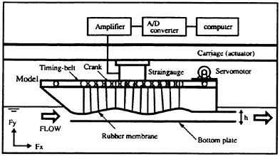
Fig. 1 Experimental set-up for the measuring force.
Fig. 2 The photograph of experiment for measuring force.
Table 1 Experimental conditions for measuring force
|
kinematic viscosity (m2/s) |
phase velocity (m/s) |
model speed (m/s) |
|
3.96×10⁻⁵ |
0.24 |
0 |
|
0.48 |
0.02 |
|
|
0.72 |
0.03 |
|
|
|
0.04 |
|
|
2.38×10⁻³ |
0.12 |
0 |
|
0.24 |
0.005 |
|
|
0.32 |
0.010 |
|
|
|
0.015 |
dynamometer is installed to the model for the measurement of force. Fig. 2 is a picture of the experimental arrangement.
A sinusoidal motion is applied to the waving surface whose amplitude and wave length (λ) are 0.01 m and 0.24 m respectively. The depth, dis-
tance between the waving surface and the bottom of model (h) is 0.02 m. The experimental conditions of carriage speed, phase velocity of wave and viscosity are tabulated in Table 1. Glycerin is used as a highly viscous fluid. Reynolds number is defined as ![]() (Vp: phase velocity of moving surface, h: depth of the bottom of model, ν: kinematic viscosity). Measurements are carried out at the sampling frequency of 500 Hz and the number of sampling data is 3000.
(Vp: phase velocity of moving surface, h: depth of the bottom of model, ν: kinematic viscosity). Measurements are carried out at the sampling frequency of 500 Hz and the number of sampling data is 3000.
Secondly, the velocity of the disturbed fluid around the waving surface is measured at small circulating water channel (L×B×D=0.6 m×0.3 m× 0.25 m) which is made for the present experiment. The maximum amplitude of sinusoidal motion is set to be 0.01 m and wave length (λ)=0.18 m/s while the phase velocity (Vp) is 0.36 m/s. Measurement are carried out for two depths of 0.03 m (h/λ=1/6) and 0.06 m (h/λ=1/3) to study the effect of shallowness.
Fig. 3 shows the experimental apparatus for the measurement of the flow field. A partickle tracking velocimetry (PTV) is used for the measurement of disturbed velocity under the waving surface. Spherical air bubbles are applied as tracers. This is because as the space between the moving surface and the bottom plate is so narrow (0.03 m~0.06 m), it is difficult for solid particles to be inserted into the measuring domain. The bottom plate is set to control the variation of depth. 50% glycerin is used as a highly viscous fluid where the kinematic viscosity is 9.2×10⁻⁵ (m2/s) and density is
The density distribution of tracers is shown in Fig. 4. Although the tracer density at the both side ends is not enough for the measurement, it is sufficient around the middle part of model where the measurement is carried out. The measuring domain is set to be from 0.25 m to 0.35 m and the breadth (in z direction) is 0.1 m (total breadth: 0.3 m) The effects of buoyancy and centrifugal force for air bubbles are removed and the sampling is being carried out during 20 seconds and mean velocity is calculated from each recorded frames.
2.2 Results
Figure 5 shows the measured force of sinusoidal motion where the model is fixed where −Fx means positive propulsive force. As the phase velocity (Vp) becomes larger, the propulsive force also becomes larger as expectation. In higher viscosity (ν=2.38×
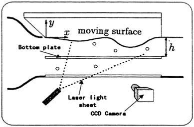
Fig. 3 Arrangement of experimental apparatus for measuring velocity.
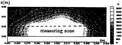
Fig. 4 Density distribution of air bubbles.
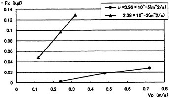
Fig. 5 Measured force acting on the model according to the variation of phase velocity at model speed of zero.
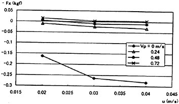
Fig. 6 Measured force acting on the model according to the variation of model speed at ν=3.96× 10⁻⁵m2/s
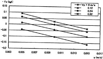
Fig. 7 Measured force acting on the model according to the variation of the model speed at ν=2.38×10⁻³m2/s
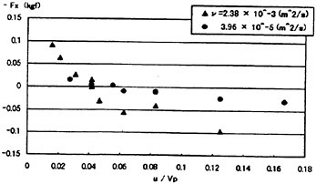
Fig. 8 Measured force acting on the model according to the ratio (u/Vp) of model speed and phase velocity.
10−3m2/s), the force and its increasing rate to Vp are larger than in those of the lower viscosity (ν=3.97×10⁻⁵m2/s).
The results of self propulsion test are summarized in Figs. 6 and 7 where u is the model speed. Although the linearity of force variation according to the model spped is not clearly seen in Fig. 6 (ν=3.97×10⁻⁵m2/s), it is clearly shown in Fig. 7 (ν=2.38×10⁻³m2/s). Fig. 7 also shows that according to the phase velocity, the space between each line is almost linear.
Figure 8 shows the variation of force according to the ratio of model speed and phase velocity (u/Vp). The propulsive force can be obtained for the ratio less than about 0.05. This means that the phase velocity of waving surface should be over 20 times the model speed for the forward move. Actually, some micro organisms, for example a flagel-late move their flagellum with very high frequency which is more than 70Hz [2]. In that case, the ratio of the forward speed and the frequency of flagellum is about 13. It might be easily guessed that the efficiency of micro organisms is very low because of sticky fluid around them even though they can move forward by their whole body working.
The average velocity profiles around waving surface are shown in Fig. 9 which are obtained from sequentially measured frames during 20 seconds. The model is fixed during the experiment. As expected, the magnitude of mean velocity in shallower case (h=0.03 m) is larger than that of deeper case (h=0.06 m). The magnitude of the mean velocity near waving surface is larger than that near the bottom plate, whose tendency is more clearly seen in the deeper case (h=0.06 m).
The variation of velocity vectors is shown in Fig. 10 during one cycle compared with computed results. The computation is carried out in two dimension with infinite model breadth while measurements are carried out on the center plane of the model. Although the magnitude of the computed velocity vectors is a little larger than that of experiment on the whole, however the directions of velocity vectors show good agreement. As the size of measuring window is only 0.1 m×0.03 m, the upper part (above y=0) of sinusoidal motion is not seen in Fig. 10. The streamlines are plotted by interpolating the measured instant velocities. The uphill part of waving surface push the fluid downward while the downhill part pull the fluid upward. By these iterative action, the fluid is resultantly
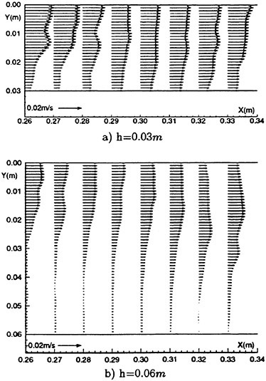
Fig. 9 Measured mean velocity distribution.
pushed forward (from left to right). The mean flux is tabulated in Table 2. The positive averaged mean flux means that fluid is pushed forward by the peristaltic motion and the moving surface obtains a propulsive force by its reaction. Although a quantitative difference is found between the computation and the experiment in Table 2, both are giving larger thrust for the shallower case.
3 Scheme and Validation for Numerical Simulation
3.1 Formulation with artificial compressibility
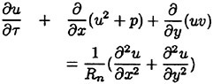
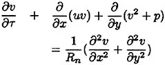
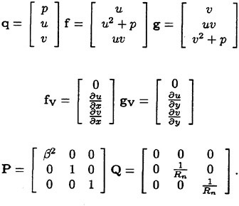
Two-dimensional incompressible Navier-Stokes equa tions are employed as governing equations which are expressed in the non-dimensional conservative form in Cartesian coordinates (x, y). Steady equa
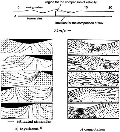
Fig. 10 Comparison of velocity vectors between the experiment and the computation (figures shown at every 60° increment over a period).
Table 2 x-directional mean flux at x=10(unit: m2/s).
|
cases |
computation |
experiment |
|
depth 0.03 m |
0.599 |
0.418 |
|
depth 0.06 m |
0.538 |
0.331 |
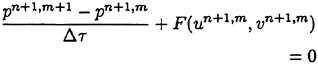
tions with artificial compressibility terms are as follows:
(1)
(2)
(3)
where τ is pseudo-time, (u, υ) are velocity components and p is pressure. The variables are normalized by principal velocity U and length L. The Reynolds number Rn is defined as ![]() where ν is kinematic viscosity. β2 is an artificial compressibility parameter defined as
where ν is kinematic viscosity. β2 is an artificial compressibility parameter defined as
where γb is a global constant and the parameter ![]() is used to prevent β2 from approaching zero near the stagnation point. γb=5 and
is used to prevent β2 from approaching zero near the stagnation point. γb=5 and ![]() =0.0001 are used in the present computations.
=0.0001 are used in the present computations.
When the solution reaches to be converged, namely ![]() becomes almost zero, the equation (1) gets the same as the original continuity equation. Equations (1)~(3) can be rewritten in the vector form as
becomes almost zero, the equation (1) gets the same as the original continuity equation. Equations (1)~(3) can be rewritten in the vector form as
(4)
where,
3.2 Spatial discretization
The fluid domain is discretized by triangular elements, and the flow variables (u, υ) and p are defined at the vertices of each triangle. The control volume for a given node i is taken as the union of all the triangles which share that node as a vertex and point k is defined as the center point of edges between point j and point j+1 as shown in Fig. 11.
The integration of the governing equation (4) over this control volume yields
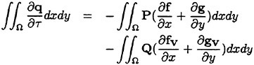
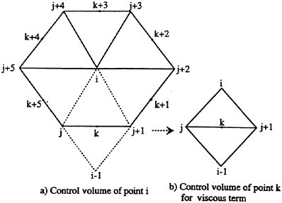
Fig. 11 Geometric identification of the control volume.
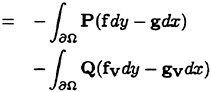
(5)
where Ω is the control volume and ∂Ω is its boundary.
In the discrete form, equation (5) can be written as
(6)
where,
Si is the area of the control volume around the node i, ne is the number of edges, (xj, yj) is the coordinate at the node j and fk and gk are the flux vector evaluated by taking average of the values at both ends of the edge, fVk is computed by the following relation,
(7)
where Ak is the area of the two triangles associated with point k as shown in Fig. 11. gVk is evaluated in the same way. In the boundary region, image points are added to the interior of boundary for the computation of terms fVk and gVk.
As the present discretization corresponds to the central difference scheme in the structured grid case, it is not stable due to the decoupling of neighboring node unless an artificial dissipation term is added to the equation. To keep the second order accuracy of the scheme, a fourth-order dissipation term is used in the scheme, which has been successfully applied to the incompressible Navier-Stokes equations [7].
3.3 Unsteady scheme and transport theorem
The unsteady numerical scheme which has been successfully established by Soh [8] with finite difference method and structured grid, is applied in the present unstructured grid scheme. The discretized equations for unsteady problem are shown in equations (8)~(10)
(8)
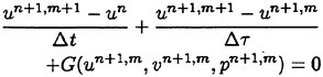
(9)
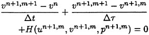
(10)
where double time loops exist; Δt and Δτ are the physical time step and the pseudo-time step due to introduction of the artificial compressibility respectively, m and n are the step number for pseudotime (τ) and the step number for physical time (t) respectively. F, G, H are residual functions of Navier-Stokes equations. The initial condition for the pseudo time loop is
where (un, υn) are converged value at physical time step n. Iteration of the computation is continued until converged at every physical time step.
For the analysis of moving problem, the effect due to the movement of control volume should be considered. Spatial integration of the Navier-Stokes equation over the control volume around cell i gives the following equations,
(11)
where Vi is the control volume and
By the transport theorem [10], the time derivative of the volume integral is given by
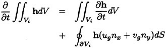
(12)
where ∂Vi is the edges surrounding the control volume of cell i. (nx, ny) and (ug, υg) are (x, y) components of the outward unit normal vector of ∂Vi and the grid velocity, respectively. The effect of the movement of control volume is considered by equation (12).
3.4 Validation
An oscillation of a plane below a viscous fluid is computed to validate the developed unsteady code, which is known as Stoke’s second problem (see, for example, White [11]). The analytic solution for the x-component velocity u, is given by
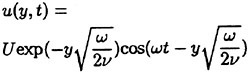
(13)
where the x-axis and y-axis are along and normal to the plate respectively, ω is frequency and ν is kinematic viscosity. Although this is a one-dimensional problem with no gradients in the direction parallel to the plate, the problem is assumed, in the present
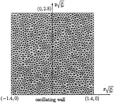
Fig. 12 Generated grid for an oscillating wall below a viscous fluid.
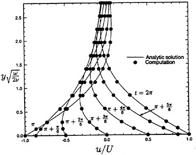
Fig. 13 Velocity profiles due to an oscillating wall (curves shown for every 30° increment over half a period).
study, to be two-dimensional to validate the developed code.
The generated grid is shown in Fig. 12. The maximum velocity of the oscillating plate (U) is set
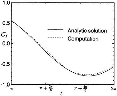
Fig. 14 Shearing stress on the oscillating wall during a half cycle.
to unity, the frequency (ω) is set to be π, and the viscosity (ν) is 0.2 m2/s in the present computation. The number of physical time step (Δt) per a cycle is set to be 60 and the number of pseudo-time (τ) iteration is 2500. The velocity profiles at x=0 at different times during a cycle are compared between the computed result and analytic solution in Fig. 13. An excellent agreement is seen between the two.
Fig. 14 shows the comparison of the shearing stress (τw) on the wall of the oscillating plane where the analytic solution is given by
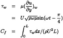
(14)
where μ is molecular viscosity, ρ is density and L is the length of plate. Although the velocity of computation is well correspondent with that of the analytic solution, there is a little difference in normalized frictional force (Cf). That is probably due to the error of numerical treatment for the computation of ![]() . In the following computations,
. In the following computations,
normalized pressure force (Cp) is defined by the following equation:
(15)
where p* is dimensionless pressure which is defined as ![]() .
.
4 Numerical Study for Peristaltic Motion
Although valuable experimental data have been obtained as mentioned in the section 2, a precise study on the flow or the propulsive force is expected which is done here by numerical simulation. The computing conditions are set to be the same as the experimental conditions for a correlative study.
A sinusoidal motion given by the equation of
(16)
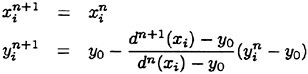
is imposed on the moving surface. For the amplitude (A(x)), a window function is used to match the moving part with the fixed part. Matching zone (LD) is set to be 10% of the length (L) of moving surface and the third order polynomial is used for matching functions in the matching zone as follows;
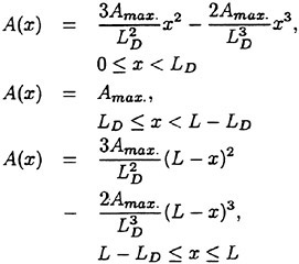
(17)
The Reynolds number ![]() is defined by the phase velocity
is defined by the phase velocity ![]() of moving surface and the depth (h) which is the distance between the moving surface and the bottom plate. The length scale is nondimensionlized by the depth h for the numerical computation.
of moving surface and the depth (h) which is the distance between the moving surface and the bottom plate. The length scale is nondimensionlized by the depth h for the numerical computation.
The generated grid below the moving surface is proportionally shrunk or stretched according to the change of distance between the moving surface and the bottom.
(18)
where d(xi) is the length between the moving surface (y0) and the bottom plate at x=xi.
The computation of the force acting on the model is first carried out in two dimension for the comparison of the experiments, The case of zero-speed condition (u/Vp=0) is typically adopted for the present computation. The generated grid for the simulation is shown in Fig. 15. Zero-gradient condition is imposed as pressure boundary condition and the x-directional velocity at outer boundary is set to be the model speed. The number of physical time step (Δt) per a cycle and the local iteration number is set to be 40 and 6000, respectively. In the present coordinate system, negative force and positive force in x-direction mean propulsive force (thrust) and drag, respectively.
Fig. 15 Generated grid for the computation of force.
Table 3 Computed x-directional forces for zero-speed condition.
|
Rn |
u/Vp |
Cf |
Cp |
Ct(Cf+Cp) |
|
2 |
0 |
5.046 |
−16.69 |
−11.64 |
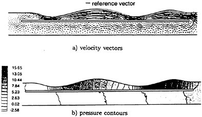
Fig. 16 Computed velocity vectors and pressure contours at after 5 cycles of computing time.
Computed results are shown in Table 3 where the total force is decomposed into the pressure and the frictional components. It is found that the pressure force is acting as a propulsive force (minus value), while the frictional force is acting as a drag. The portion of pressure force is greater than that of frictional force, which makes a propulsive force resultantly. Computed velocity vectors and pressure contours are shown in Fig. 16 which are obtained after 5 cycles of motion. The disturbed velocity by the waving surface is clearly seen in the figure of velocity vectors and the difference of pressure between the uphill region and the downhill region is also seen in the profile of pressure contour. It is found that the difference of pressure makes the waving surface produce a thrus force.
Figure 17 shows the generated grid for the computation of velocity field. Simulations are carried out for the two depths (h) of 0.03 m and 0.06 m. The corresponding Reynolds numbers are 117 and 234, respectively. The zero-gradient is imposed on the boundary condition of pressure while the velocity is zero at the outer boundary.
For the case of depth 0.06 m, the computation of forces acting on the moving surface is carried out for the validation of the present computation. The computation is continued over ten full periods after which the forces are fully periodic in time as shown in Fig. 18. In this case the frictional force acting on the bottom plate is not included in the total frictional force. The number of physical time step (Δt) per a cycle and the local iteration (m loop) are 30 and 4000 respectively. As shown in Fig. 18, the rate
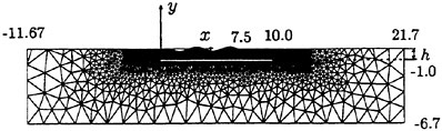
Fig. 17 Generated grid of depth 0.06 m for the computation of contractive and dilative motion of surface.
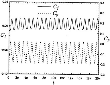
Fig. 18 The profiles of frictional force and pressure force according to the computing time.
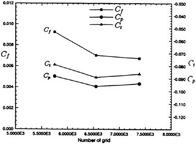
Fig. 19 Computed x-directional mean forces for the case of depth 0.06 m according to the variation of grid number.
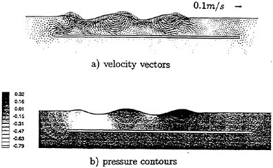
Fig. 20 Computed velocity vectors and pressure contours for the case of depth 0.06 m at after 5 cycles of computing time.
of periodic convergency is so fast that about 5 cycles are enough to reach the periodically convergent state. The dependency of the mean forces on the grid number is shown in Fig. 19 where the negative force means the propulsive force. Beyond 6.5×10³ grid, the dependency becomes less.
The velocity vectors and pressure contours at after 5-th cycle are shown in Fig. 20. The difference of pressure between on the uphill and on the downhill acts as a propulsive force. The computed velocity vectors of the case of depth 0.03 m are shown in Fig. 10 compared with those of experiment. The mean flux at the section of x=10 is compared in Table 2. The positive mean flux means that propulsive force can be obtained by such a type of sinusoidal motion of the moving surface as given by equation (16).
From the present simulations, it is proved that a propulsive force is produced dominantly by the pressure force component with the sinusoidal motion of the moving surface in shallow water condition.
5 Contractive and Dilative Motion
For further application a contractive and dilative motion, shown in Fig. 21, is numerically studied. As the body is symmetry, a half plane is used for the computation. The middle part of the body makes
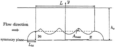
Fig. 21 Schematic for the description of the contractive and dilative motion of body.
a contractive and dilative motion which seems a worm-like motion, while the head and tail parts are not movable. The Reynolds number ![]() is defined by the length (L) of the movable part and the phase velocity
is defined by the length (L) of the movable part and the phase velocity ![]() of motion. All the lengths are non-dimensionalized by the length (L) of movable part of body. Two types of motion are studied for the moving surface of body, which are sinusoidal and trochoidal motions given by equations (19), (20) and (21) respectively.
of motion. All the lengths are non-dimensionalized by the length (L) of movable part of body. Two types of motion are studied for the moving surface of body, which are sinusoidal and trochoidal motions given by equations (19), (20) and (21) respectively.
sinusoidal motion:
(19)
trochoidal motion:
(20)
(21)
In the present study, the parameters for motions are set as ![]()
![]() b=0.5 and yo(=Lht)=0.15. For the amplitude (A(x)), the window function given by equation (17) is used. As shown in equations (19)~(21), the direction of the phase of sinusoidal motion is reverse to the advancing of the body while the trochoidal case is the same.
b=0.5 and yo(=Lht)=0.15. For the amplitude (A(x)), the window function given by equation (17) is used. As shown in equations (19)~(21), the direction of the phase of sinusoidal motion is reverse to the advancing of the body while the trochoidal case is the same.
The generated grid system above the moving surface is proportionally shrunk or stretched according to the change of the distance between the moving surface and the top as given by following equations.
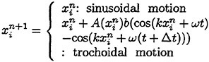
(22)
where d(xi) is the length between the base of body surface (yu) and the top location (ho) at x=xi.
5.1 Unbounded case
Computations are carried out for the unbounded fluid to study how propulsive force is acting on a body by the contractive and dilative motion. Generated grid for unbounded fluid case is shown in Fig. 22. The phase velocity of the moving surface is ten times the oncoming velocity. The number of physical time step (Δt) per a cycle is set to be 60 and the number of iteration for pseudo time is 3000.
Computations are carried out for the sinusoidal motion and the trochoidal motion at three different Reynolds numbers of 5, 50 and 500.
As the direction of sinusoidal motion is the same as that of on-coming flow, the pressure force can act as a propulsive force as shown in Table 4. As the frictional force is comparatively larger than the pressure force at ![]() it is difficult to obtain a propulsive force by the sinusoidal motion. The sinusoidal motion is more precisely discussed for the narrow channel case in the next section.
it is difficult to obtain a propulsive force by the sinusoidal motion. The sinusoidal motion is more precisely discussed for the narrow channel case in the next section.
The computed x-directional mean forces for the trochoidal motion are also tabulated in Table 4. The computing conditions are the same as the sinusoidal case. Contrarily to the sinusoidal case, the portion of the frictional force becomes larger as the Reynolds number becomes lower. The total force (Ct) of the frictional force (Cf) and the pressure force (Cp) is largely negative at ![]() which means that the body can move forward faster more than 10% of its phase velocity. This situation is clearly demonstrated in the computed velocity vectors and pressure contours shown in Fig. 23 where the peak value is intentionally cut off to express the intermediate distribution more clearly. Although the difference of the pressure between on the downhill and on the uphill is acting as a drag to the body, the flow above the moving surface rotated by the trochoidal motion of surface produces a propulsive force to body.
which means that the body can move forward faster more than 10% of its phase velocity. This situation is clearly demonstrated in the computed velocity vectors and pressure contours shown in Fig. 23 where the peak value is intentionally cut off to express the intermediate distribution more clearly. Although the difference of the pressure between on the downhill and on the uphill is acting as a drag to the body, the flow above the moving surface rotated by the trochoidal motion of surface produces a propulsive force to body.
Through the present simulations, it can be concluded that a contractive and dilative motion with a trochoidal motion of surface can produce a propul-
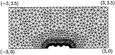
Fig. 22 Generated grid for the computation of trochoidal motion in unbounded fluid.
Table 4 Computed results of x-directional forces of the body in unbounded fluid.
|
Conditions |
Cf |
Cp |
Ct |
|
|
sinusoidal motion |
|
7.510 |
−3.584 |
3.926 |
|
|
0.704 |
−0.612 |
−0.092 |
|
|
|
0.047 |
−0.224 |
−0.177 |
|
|
trochoidal motion |
|
−8.119 |
4.541 |
−3.578 |
|
|
−0.744 |
0.807 |
0.063 |
|
|
|
−0.052 |
0.383 |
0.331 |
|
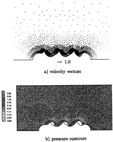
Fig. 23 Computed velocity vectors and pressure contours around the body in unbounded fluid with the trochoidal motion at after 5 cycles of computing time.
sive force in unbounded fluid if Reynolds number is low (![]() under the present computing conditions).
under the present computing conditions).
5.2 Narrow channel case
Numerical studies are further extended to the case for a body in narrow channel. The generated grid for the computation is shown in Fig. 24. This case is more practical in imaging that a worm-like body propels in a tube filled with highly viscous fluid. The half breadth of the narrow channel is set to be 0.55L (L: movable length of body) and the magnitude of on-coming velocity is one tenth the phase velocity of the body surface motion.
The computed x-directional mean forces at three different Reynolds numbers are tabulated in Table 5. In the case of high Reynolds number flow, a propulsive force can be obtained by the pressure force with the sinusoidal motion, while the portion of frictional force becomes larger to act as a larger drag at lower Reynolds number. The tendency is almost the same as that confirmed for the unbounded case. The computed velocity vectors and the pressure contours for the sinusoidal motion at ![]() are shown in Fig. 25. The pressure difference between on the downhill and on the uphill produces a propulsive force. In the sinusoidal motion, the flow on the moving surface is not rotated. This phenomenon is different from that of the trochoidal motion.
are shown in Fig. 25. The pressure difference between on the downhill and on the uphill produces a propulsive force. In the sinusoidal motion, the flow on the moving surface is not rotated. This phenomenon is different from that of the trochoidal motion.
The computed mean forces for the trochoidal motion are also shown in Table 5. The tendency according to the variation of Reynolds number is completely reverse to the case of sinusoidal motion. The portion of frictional force is smaller than that of unbounded fluid case on the whole and the frictional force can act as a propulsive force even in highly viscous flow. Computed velocity vectors and pressure contours at ![]() are plotted in Fig. 26. The rotated flow by the trochoidal motion of surface is clearly seen in the profile of velocity vectors.
are plotted in Fig. 26. The rotated flow by the trochoidal motion of surface is clearly seen in the profile of velocity vectors.
It can be concluded that the propulsive force is also obtained in highly viscous fluid of narrow channel by the firctional force if the trochoidal motion is applied to the waving surface.
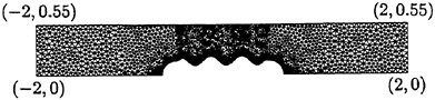
Fig. 24 Generated grid for the computation of sinusoidal motion in narrow channel
Table 5 Computed results of x-directional forces of the body in narrow channel.
|
Conditions |
Cf |
CP |
Ct |
|
|
sinusoidal motion |
|
4.120 |
−3.105 |
1.015 |
|
|
0.338 |
−0.782 |
−0.444 |
|
|
|
0.029 |
−0.294 |
−0.266 |
|
|
trochoidal motion |
|
−5.117 |
3.777 |
−1.340 |
|
|
−0.432 |
0.788 |
0.356 |
|
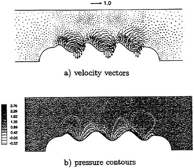
Fig. 25 Computed velocity vectors and pressure contours around the body in narrow channel with the sinusoidal motion at after 5 cycles of computing time.
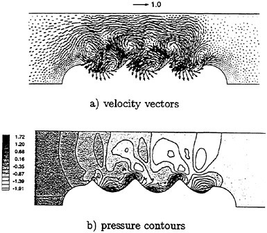
Fig. 26 Computed velocity vectors and pressure contours around the body in narrow channel with the trochoidal motion at after 5 cycles of computing time.
6 Concluding remarks
A propulsion system by peristaltic motion in highly viscous fluid is studied by experimentally and numerically. The experimental results of self propulsion test show that if the phase velocity of sinusoidal motion of the body surface is over 20 times the model speed, the model can successfully advance in highly viscous fluid by peristaltic motion. The velocity measurement by the particle tracking velocimetry disclosed that fluids are more effectively transported for the case of narrower clearnce between the body surface and the bottom because the difference of pressure plays a role in transportation. This is clearly proved by numerical computation also. It is experimentally concluded that a propulsion system by peristaltic motion can be applied as a propulsor in highly viscous fluid.
Numerical studies carried out to investigate the mechanism of peristaltic motion more closely show that the pressure force is acting as a propulsive force in the peristaltic motion. Although some quantitative difference is found between the computation and the experiment, the tendency is rather similiar each other.
For the application to the micro-hydro machine, the present study is extended to a contractive and dilative motion of body. Propulsive force can be obtained in highly viscous fluid by a contractive and dilative motion of body. The trochoidal motion makes the fluid rotate to obtain propulsive force, while the sinusoidal motion makes the difference of pressure by which propulsive force is obtained. In highly viscous flow, the frictional force acts as propulsive force in a narrow channel.
By the present study, it is clearly mentioned that a propulsive force can be obtained in highly viscous fluid either by sinusoidal or trochoidal motion. The sinusoidal motion is effective in the case of shallow water, while the trochoidal is in extremely low Reynolds number fluid. The present study is expected to be applied for the development of a propulsor for micro-hydro machine and further studies may provide more efficient way of motion for the production of thrusting force.
References
[1] A.Azuma, “The Biokinetics of Flying and Swimming,” Springer-Verlag, Tokyo, 1992. pp. 1–4, pp. 163–164.
[2] R.M.Alexander, “Exploring Biomechanics (animal in Motion),” W.H.FREEMAN AND COMPANY, 1992, pp. 213–218.
[3] A.Azuma, “The Mechanism on Swimming of Organism,” Blue Backs, 1980, pp. 147–151.
[4] F.C.P.Yin and Y.C.Fung, “Comparison Theory and Experiment in Peristaltic Transport,” Journal of Fluid Mechanics, Vol. 47, 1971, pp. 93–112.
[5] S.Ninomiya and T.Mizutani, “The Visualization Analysis of High Viscous Flow Field Induced by Peristaltic Propelling Device,” Journal of the Visualization Society of Japan, Vol. 17, No. 1, 1997, pp. 249–252.
[6] M.-C.Kim, K.Mori, Y.Doi and Q.Xu, “A Numerical Study on Propulsive Force by Contractive and Dilative Motion in Highly Viscous Fluid,” Journal of the Society of Naval Architects of Japan, Vol 183, No. 1, 1998, pp. 27–33.
[7] M.-C.Kim, K.Mori, Q.Xu and Y.Doi, “A Numerical Scheme with Unstructured Mov-
ing Grid System and its Application to Two-Dimensional Complicated Flow,” Journal of the Society of Naval Architects of Japan, Vol. 181, 1997, pp. 45–53.
[8] W.Y.Soh, “Unsteady Solution of Incompressible Navier-Stokes Equations,” Journal of Computational Physics, Vol. 79, 1988, pp. 134–134.
[9] J.C.Cavendish, “Automatic Triangulation of Arbitrary Planar Domains for the Finite Element Method,” International Journal for Numerical Method in Engineering, Vol. 8, 1974, pp. 679–696.
[10] J.N.Newman, “Marine Hydrodynamics,” The MIT Press, 1977, pp. 57–59.
[11] F.M.White, “Viscous Fluid Flow,” McGraw-Hill, New York, 1974, pp. 148–149.
DISCUSSION
Naomi Kato, Japan
1. An earthworm moves on the ground by peristaltic motion of its own body. The discusser thinks that “peristaltic motion” of body means the contractive and dilative motion of body on the ground. It would be valuable if the authors could show the relationship between the propulsive force and the distance (h) of the moving surface from the bottom plate including h of zero, in the experimental study by use of a mechanism producing peristaltic motion.
2. Please show the propulsive efficiency of the device shown in Fig. 1.
3. How do you estimate three-dimensional effect of the flow around the device experimentally in comparison with the computational results in two-dimensions as shown in Table 2?
4. Vaidyanathan [1] recently has developed a hydrostatic robot that is 16 cm long and can move on the ground in water at 0.7 cm/s. It consists of three segments. Each segment consists of two solid circular discs connected by four equidistant shape memory alloy springs. A fluid filled bladder in the center of each segment provides hydrostatic skeletal support. What kind of device is needed in practice in your research to produce contractive and dilative motion in low Reynolds numbers as shown in Table 4?
[1] Vaidyanathan, R., “Hydrostatic Robot for Marine Applications,” Video Proc. of 1998 IEEE International Conference on Robotics and Automation, 1998
AUTHORS’ REPLY
1. We studied the effect of depth (h) which was the distance between the waving surface and the bottom plate (see Fig. 9 and Table 2). Unfortunately, only two kinds of depth were treated in the experiment of velocity measurement. Although the computational results of propulsive force were not shown in the paper, the absolute value of the propulsive force of shallower water (0.03 m) is about 1.5 times that of the deeper case (0.06 m). For the case of h of zero, both the experiment and the computation are not easy to be carried out.
2. Because of the difficulty of open water test for the present device, we did not derive the efficiency of the self-propulsion test. The efficiency is not the main purpose of the present paper.
3. In the present study, the three dimensional effects are not included in the computational results. Three dimensional code is expected to be developed for the more precise comparison.
4. The experiments for peristalic motion with trochoidal movement is under consideration. We have carried out preliminary experiment for the micro-hydro-machine by using of magnetic mechanism, but we could not obtain satisfactory results. It is our keen interest to apply the finding to a micro-hydro-machine.
DISCUSSION
C.Johannsen
Hamburg Ship Model Basin, Germany
Can the author give us an idea about the overall efficiency of the peristaltic propulsion system in comparison to a conventional propeller drive? This would be interesting especially for the viscosity of sea water.
AUTHORS’ REPLY
In the extremely low Reynolds number fluid, obtaining a propulsive force is very difficult by conventional propulsion system. In the present study, the possibility of obtaining a propulsive force is demonstrated by the proposed contractive and dilative motion. The efficiency is expected as the secondary importance here.
A New Surface Panel Method to Predict Steady and Unsteady Characteristics of Marine Propeller
J.Ando,1 S.Maita,2 K.Nakatake1
(1Kyushu University, 2West Japan Fluid Engineering Lab. Co. Ltd., Japan)
ABSTRACT
This paper presents a new surface panel method “SQCM” which satisfies easily the Kutta condition. First the fundamental equations and numerical procedure of SQCM are described. Next the calculated results for the 2-D steady and unsteady wing problems are shown and the accuracy of SQCM is discussed emphasizing the wing thickness effects on the calculated results. Then the steady and unsteady calculations for Seiun-Maru conventional and highly skewed propellers are made, and the calculated pressure distributions on the propeller blades and the propeller open characteristics are compared to the experimental data. Finally the shaft forces and moments of DTMB P4118 are shown and some discussions are made.
1. INTRODUCTION
As the methods to obtain the flow field around thick wing, the Hess’ [1] and Morino’s [2] panel methods are often used. These methods represent the flow field around a wing by the source and the doublet distributions on the wing surface, and are applied successfully to calculation of the pressure distribution on the propeller blade. But it is not so easy to satisfy the Kutta condition at the tailing edge and many discussions were raised about it (Koyama [3]). A reasonable expression of the Kutta condition is that the pressure becomes equal on the upper and the lower wing surfaces at the tailing edge. In order to satisfy the above condition, it is needed to solve iteratively the quadratic simultaneous equations for singularity distributions.
Recently we developed a new surface panel method which is a kind of singularity method. This method uses source distributions (Hess and Smith [4]) on the wing surface and discrete vortex distributions arranged on the camber surface according to quasi-continuous vortex lattice method (QCM) (Lan [5]) (see Fig. 1). Then these singularities are determined at a time by solving simultaneously both the wing surface and the camber surface conditions that the normal velocity should be zero in case of the steady problem. Since these singularities satisfy automatically the Kutta condition, we need not use any iterative procedure. In case of the unsteady problem, we introduce the normal velocity to the camber surface at the trailing edge in order to make the pressure difference between the upper and the lower wing surfaces zero. Even though the iterative procedure to satisfy the Kutta condition is necessary, the convergence is quite fast. We named this simple surface panel method SQCM (Source and QCM).
The calculated results of SQCM for 2-D and 3-D wings, steady propeller problem and unsteady propeller problem have been presented by Nakatake et al. [6], Ando et al. [7] and Maita et al. [8], respectively.
In this paper we describe the fundamental equations and numerical procedure of SQCM and the steady results of Seiun-Maru propellers and the unsteady results of Seiun-Maru propellers and the results of shaft forces and moments of DTMB P4118.
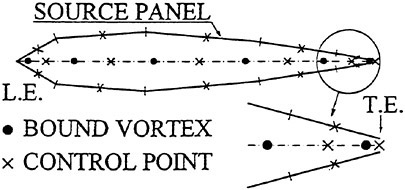
Fig. 1 Arrangement of source panels, bound vortices and control points
2. FUNDAMENTAL EQUATIONS AND NUMERICAL PROCEDURE OF SQCM
2.1 General
In this chapter, basic equations and numerical procedure of SQCM in the unsteady case are mainly described. At first we mention the outline of SQCM, then show the velocity potential to express the flow around a propeller, the boundary conditions including the Kutta condition and the numerical procedure.
In SQCM, the upper and the lower surfaces of the propeller blades are divided into the same numbers of source panels, respectively. Then the ring vortices are located on the mean camber surface according to the unsteady QCM (Hoshino [9]) (Murakami et al. [10]). The hub surface is also divided into source panels. The trailing vortices flow out as ring vortices from the trailing edge every time step. We assume that the trailing vortices leave the trailing edge in the direction tangential to the mean camber surfaces and the pitch of trailing vortices reaches an ultimate value, which is the mean of geometrical pitch distribution of the propeller blade, within a half revolution.
We solve the boundary conditions every time step Δt. The source distributions on propeller blades and hub surface and the vortex distributions on the camber surfaces are obtained for each time step from the boundary conditions at the center of the source panels and the control points on camber surfaces whose positions are determined by the QCM theory. Here the pressure Kutta condition is considered simultaneously.
The perturbation potentials and velocity distributions on the blade surfaces are obtained from these singularity distributions. The pressure distributions are calculated by the unsteady Bernoulli’s equation. Then the forces acting on propeller blades are obtained by pressure integration on the propeller blade.
2.2 Velocity Vector
Consider a K-bladed propeller rotating with a constant angular velocity Ω in inviscid, irrotational and incompressible fluid. The space coordinate system Ο-XYZ and the propeller coordinate system Ο-xyz are introduced as Fig. 2.
The propeller blade SB is divided into Μ panels in the spanwise direction. The face and the back sides of the blade section are divided into Νσ panels in the chordwise direction, respectively. Therefore the total number of source panels for each blade surface becomes Μ×2Νσ and constant source in each panel is distributed. The hub surface SH is also divided into quadrilateral panels. The velocity vector Vσ due to the source distributions on the blade and hub surfaces is expressed by using the velocity potential Φσ as
(1)
where
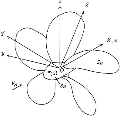
Fig. 2 Coordinate systems of propeller
Next the mean camber surface is divided into Μ segments in the spanwise direction corresponding to the division of the source panels and divided into Νγ in the chordwise direction. Here we introduce ξ axis whose origin locates at the leading edge and is extended to the trailing vortex surface along the mean camber surface. The positions of the bound vortex ![]() and control point
and control point ![]() on the mean camber surface are expressed by the following equations according to the QCM theory.
on the mean camber surface are expressed by the following equations according to the QCM theory.

(2)
where
μ and ν are the numbers in the spanwise and chordwise directions. ξL(rμ) and ξT(rμ) are the positions of the leading edge (L.E.) and trailing edge (T.E.), respectively. And total Μ×Νγ ring vortices are located on the mean
camber surface according to Eq. (2) as illustrated in Fig. 3. One set of ring vortices consists of one bound vortex, two free vortices and the first spanwise shed vortex CH closest to the trailing edge in the trailing wake. In case of the unsteady problem the shed vortex flows out from T.E. Thus the ring vortex which represents the shed vortex is located in the trailing wake. This ring vortex consists of two spanwise shed vortices CH, EF and two streamwise trailing vortices CE, HF. Here we define the induced velocity vectors due to the ν′-th ring vortex of unit strength which starts from the μ-th strip and ones due to the l-th ring vortex of unit strength located in the trailing wake as ![]() and
and ![]() respectively. These induced velocity vectors are expressed as
respectively. These induced velocity vectors are expressed as
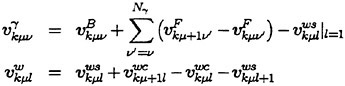
(3)
where
![]() =induced velocity vector due to the bound vortex of unit strength on the mean camber surface
=induced velocity vector due to the bound vortex of unit strength on the mean camber surface
![]() =induced velocity vector due to the free vortex of unit strength on the mean camber surface
=induced velocity vector due to the free vortex of unit strength on the mean camber surface
![]() =induced velocity vector due to the spanwise shed vortex of unit strength in the trailing wake
=induced velocity vector due to the spanwise shed vortex of unit strength in the trailing wake
![]() =induced velocity vector due to the streamwise trailing vortex of unit strength in the trailing wake
=induced velocity vector due to the streamwise trailing vortex of unit strength in the trailing wake
The induced velocity vector ν due to each line segment of vortex is calculated by the Biot-Savart law.
If we define the strengths of the ring vortex on the mean camber surface at time tL and the ring vortex in the trailing wake as γkμν(tL) and Γkμ(tL−l), the induced velocity vector due to the vortex model of the QCM theory is given by the following equation.
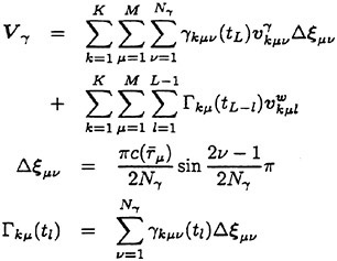
(4)
Eq. (4) is used when the control points are on the mean camber surface. When the control points are on the blade surface, the ring vortices are close to the control points especially for thin wing. In this case we treat the ring vortices on the mean camber surface and the shed vortex nearest to T.E. as the vortex surfaces in order to avoid numerical error. We call this treatment “Thin Wing Treatment” (Maita et al. [11]). Then we modify the vortex model of the QCM theory as follows:
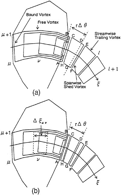
Fig. 3 Arrangement of vortex systems
First, we close the ring vortex on the mean camber surface at T.E. and locate ring vortices ABCH, HCDG and GDEF downstream form T.E. as illustrated in Fig. 3(b).
Next, we replace the ν-th ring vortex with a set of ring vortices distributed along Δξμν on the mean camber surface as illustrated in the middle of Fig. 3(b). Then the ring vortex ABCH just downstream from T.E. and the ring vortex HCDG are replaced with a set of ring vortices distributed along rΔθ in the trailing wake. The ring vortices downstream from rΔθ are calculated as discrete ring vortices.
In this case, the induced velocity vectors due to the vortex systems on the mean camber surface and in the trailing wake are expressed as
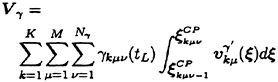
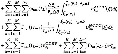
(5)
where
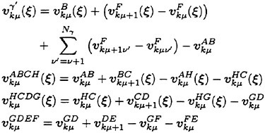
Here the first term in the right hand side of Eq. (5) is derived by “Thin Wing Treatment”, the second and third terms express the shed vortex just downstream from T.E. and the 4-, 5-th terms express other ring vortices in the trailing wake.
In this way, the velocity vector V around a propeller in the propeller coordinate system is expressed as
(6)
where VI, Vγ and Vσ are inflow, induced velocity vectors due to vortex and source distributions, respectively.
2.3 Kutta Condition
We consider that the velocity normal to the mean camber surface at T.E. is zero (VN=0) as the Kutta condition in the steady SQCM. On the other hand we introduce the normal velocity at T.E. in order to make the pressure difference between the upper and lower surfaces zero in the unsteady case. We choose the control points on the upper and the lower source panels at T.E. as the positions where the Kutta condition is satisfied. Here we define the pressure difference as Δp and indicate the upper and the lower surfaces with subscripts + and −, respectively. Defining the perturbation potential and the magnitude of velocity on the upper and lower surfaces as ![]() and V+, V−, respectively, the Kutta condition in the unsteady SQCM is given by
and V+, V−, respectively, the Kutta condition in the unsteady SQCM is given by
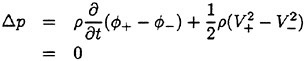
(7)
2.4 Boundary Conditions and Numerical Procedure
The boundary conditions at the control points on the blade, mean camber and hub surfaces are that there is no flow across the surfaces. But there exists at T.E. the normal velocity which is introduced to satisfy the Kutta condition as expressed by Eq. (7). Therefore the equations of the boundary conditions are given as follows:
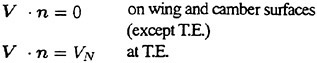
(8)
where n is the normal vector on the blade, mean camber and hub surfaces.
The unknown values are the vortex strengths on the mean camber surface, source strengths on the blade and hub surfaces and normal velocity VN at T.E.. VN is expressed by the following equation and determined so as to satisfy the Kutta condition iteratively.
(9)
Here i is the number of iteration. The first term in the right hand side in Eq. (9) means the corrector for the value of the previous step ![]() which is proportional to the pressure difference Δp(i). The iteration is continued until the pressure difference becomes small (ΔCp<0.5×10⁻³). β means the acceleration factor and β=1 in this calculation. Assuming the normal velocity VN at T.E. at each iterative step, Eq. (8) can be solved as the linear simultaneous equations for singularity distributions.
which is proportional to the pressure difference Δp(i). The iteration is continued until the pressure difference becomes small (ΔCp<0.5×10⁻³). β means the acceleration factor and β=1 in this calculation. Assuming the normal velocity VN at T.E. at each iterative step, Eq. (8) can be solved as the linear simultaneous equations for singularity distributions.
The coefficient matrix in this calculation does not change at any time step and iteration for the Kutta condition. Therefore we can reduce the computing time by storing the inverse matrix of the coefficient matrix.
The Kutta condition in the unsteady SQCM is satisfied solving the linear simultaneous equation in the same way as the steady problem. So the algorithm is simple and efficient. The typical number of iterations for the Kutta condition is about five times at each time step in the unsteady problem.
2.5 Unsteady Pressure and Propeller Forces
The unsteady pressure distribution on the propeller blade is calculated by the unsteady Bernoulli equation expressed as
(10)
where
p0=the static pressure in the undisturbed inflow
ρ=the density of the fluid
![]() =the perturbation potential in the propeller coordinate system
=the perturbation potential in the propeller coordinate system
Here the time derivative term of ![]() in Eq. (10) is obtained numerically by two points upstream difference scheme with respect to time. Before numerical differentiation the perturbation potential
in Eq. (10) is obtained numerically by two points upstream difference scheme with respect to time. Before numerical differentiation the perturbation potential ![]() is calculated analytically for source and vortex components, respectively [12].
is calculated analytically for source and vortex components, respectively [12].
The blade pressure of the propeller is expressed as the pressure coefficient Cp in order to compare the calculated results with experimental data. The pressure coefficient is defined by
(11)
where n is the rate of revolutions of the propeller and D is the diameter of the propeller.
The thrust T and the torque Q of the propeller are calculated by pressure integration. Denoting the x−, y− and z− components of the normal vector on the blade surface by nx, ny and nz, respectively, the thrust and the torque are expressed by
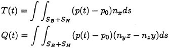
(12)
In the steady calculation the viscous components of the thrust and the torque are considered approximately according to Nakamura [13] using the viscous drag coefficient of blade element Cd at the radius r. These components TD and QD are expressed as
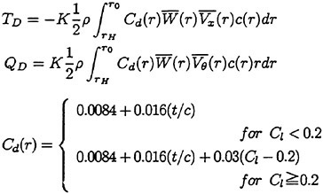
(13)
where
Cl=sectional lift coefficient
![]()
![]() =x-component of resultant flow velocity averaged in the chordwise direction
=x-component of resultant flow velocity averaged in the chordwise direction
![]() =θ-component of resultant flow velocity averaged in the chordwise direction
=θ-component of resultant flow velocity averaged in the chordwise direction
c(r)=chord length of the propeller blade
r0=propeller radius
rΗ=hub radius
t/c=thickness ratio
The forces FX, FY, FZ and moments ΜY, MZ acting on the propeller in the X, Y, Z directions of the space coordinate system are expressed as
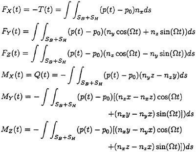
(14)
These forces and moments are nondimensionalized as follows:
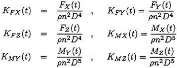
(15)
Finally the advance coefficient J, the thrust and the torque coefficients KT, KQ and the propeller efficiency ηp are expressed as follows:
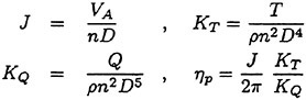
(16)
where VA is the advance velocity of the propeller.
3. CALCULATED RESULTS
3.1 2-D Steady Wing
As the first example, we calculate about the Kármán-Trefftz wings with angle of attack of 5 degrees in uniform flow. In this calculation we adopt Νσ=30 and Nγ=29. Fig. 4 shows the pressure
distribution on the symmetrical Kármán-Trefftz wing whose thickness ratio is 0.12. The pressure distribution obtained by SQCM agrees well with the analytic solution and the accuracy of SQCM is confirmed. It is also seen that the Kutta condition at the trailing edge is satisfied. Fig. 5 shows the source and vortex distributions in this calculation.
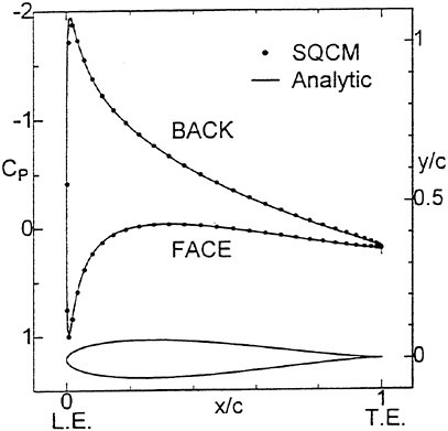
Fig. 4 Comparison of pressure distributions (Kármán-Trefftz wing)
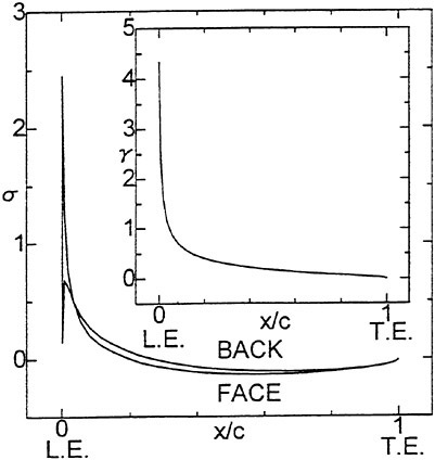
Fig. 5 Source and vortex distributions (Kármán-Trefftz wing)
In order to check the effect of the wing thickness on the SQCM solution we perform some calculations for wings with various thickness ratios. Fig. 6 shows the change of lift coefficient for Kármán-Trefftz wing with various thickness ratio and camber. The SQCM results agree well with the analytic solutions in wide range of the wing thickness even though the thickness is very thin.
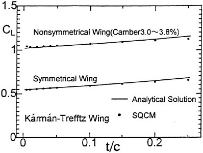
Fig. 6 Change of lift coefficient for Kármán-Trefftz wing with various thickness ratio and camber
3.2 2-D unsteady wing
The calculated results for unsteady wing problems using SQCM are described in Ref. [14] in detail. So we show here some results only in 2-D sinusoidal gust problem. We calculate the lift of wings with different thickness advancing in the sinusoidal gust whose vertical speed υ(x, t) is υ0eiν(t−xU), where ν=2πU/ℓ, ℓ is wave length of the gust and υ0 is gust amplitude. In this case, the reduced frequency k is given by πcℓ. Fig. 7 shows the time history of the lift coefficients comparing with thin wing result. A good agreement is obtained between NACA0001 and thin wing.
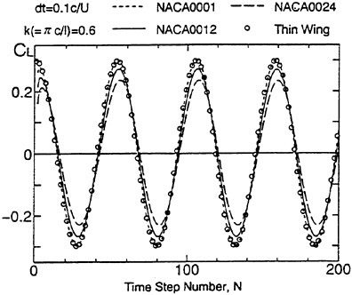
Fig. 7 Time history of lift coefficients (Sinusoidal gust)
3.3 Propeller problems
3.3.1 Seiun-Maru CP and HSP
We select the Seiun-Maru conventional propeller (CP) and highly skewed propeller (HSP) for the propeller calculations because there exist Ukon et al.’s rich experimental data [15][16][17]. The principal particulars of these propellers are shown in Table 1. The propeller blade surface and the mean camber surface are divided into 1200 panels (M=20, Νσ=30) and 580 line segments (M=20, Nγ=29), respectively, per blade for each propeller. Panel arrangements of the propellers are shown in Fig. 8.
Table. 1 Principal particulars of Seiun-Maru CP and HSP
|
NAME OF PROPELLER |
CP |
HSP |
|
DIAMETER (mm) |
400 |
400 |
|
NUMBER OF BLADE |
5 |
5 |
|
PITCH RATIO AT 0.7R |
0.95 |
0.944 |
|
EXPANDED AREA RATIO |
0.65 |
0.70 |
|
HUB RATIO |
0.1972 |
0.1972 |
|
SKEW ANGLE (DEG.) |
10.5 |
45.0 |
|
RAKE ANGLE (DEG.) |
6.0 |
−3.0 |
|
BLADE SECTION |
MAU |
MODIFIED SRI-B |
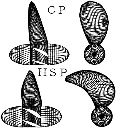
Fig. 8 Panel arrangements for Seiun-Maru CP and HSP
3.3.1.1 Steady case
The pressure distributions obtained by SQCM at 0.7R sections of Seiun-Maru CP and HSP are shown in Figs. 9 and 10 comparing with the experimental data [15] and the results of Hoshino’s panel method [18]. The SQCM results agree well with the experimental data and Hohino’s results.
The propeller characteristics of the propellers are shown in Fig. 11 and 12 comparing with the experimental data [19]. Though the viscous effects are considered approximately, the calculated results agree well with the experimental results.
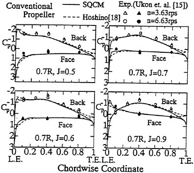
Fig. 9 Comparison of chordwise pressure distributions (Seiun-Maru CP)
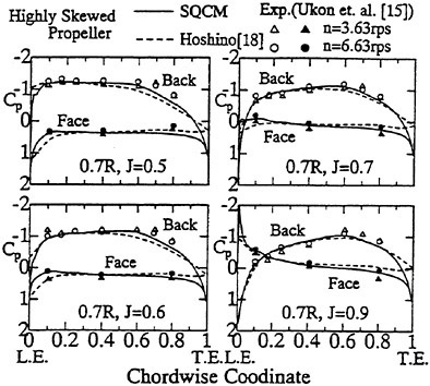
Fig. 10 Comparison of chordwise pressure distributions (Seiun-Maru HSP)
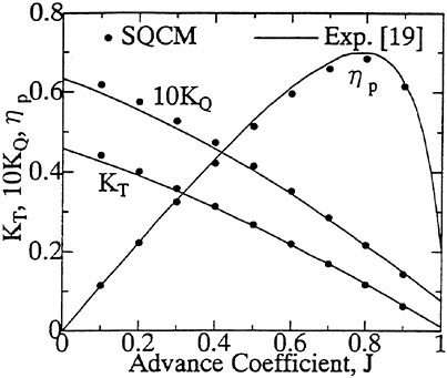
Fig. 11 Comparison of propeller characteristics (Seiun-Maru CP)
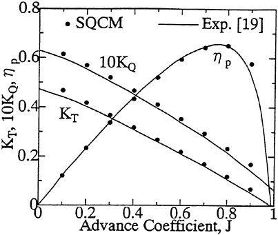
Fig. 12 Comparison of propeller characteristics (Seiun-Maru HSP)
3.3.1.2 Unsteady case
In the unsteady calculations, the time step Δt is chosen as Δθ/Ω, Δθ=6 degrees. The calculated results after five revolutions of the propeller are taken as the converged values.
The full scale measurements of the pressure distribution on the blade for Seiun-Maru CP and HSP were conducted [16][17]. Corresponding calculation is performed using the given wake distribution (see Fig. 13) estimated by Sasajima and Tanaka’s method from the wake measurements in model scale performed in a towing tank.
Comparisons of the pressure fluctuations at 0.7 and 0.9R sections during one revolution between the calculated results and the experimental data are shown in Figs. 14 and 15. The agreement between the calculated results and the experimental data is generally good except the back side of 0.8 chord of 0.9R section of HSP.
Chordwise pressure distributions at angular positions of 0, 90, 180 and 270 degrees at 0.7 and 0.9R sections are compared to the experimental data and the results of Hoshino’s panel method [20] in Figs. 16 and 17. The SQCM results at 0.7R section agree well with the experimental data. On the other hand, some discrepancies between the calculated results and the experimental data are observed on the back side at 0.9R section of HSP.
These disagreements between the calculated results and the experimental data of the pressure fluctuation and the chordwise pressure distribution on the back side at 0.9R section of HSP might be caused by the tip vortex stemmed from the leading edge separation [17].
Fig. 18 shows the calculated thrust fluctuations of CP and HSP. The wake coefficients 1−wX, wr and wθ in the axial, radial and circumferential directions of the estimated wake distribution are also shown. We can see that the thrust acting on one blade shows one period of fluctuation during one revolution but the total thrust of the five-bladed propeller shows five periods of fluctuation during one revolution. The skew effect of the propeller is confirmed in this calculation because the fluctuation of HSP is smaller than that of CP. It seems that the axial wake factor 1−wX mainly affects the thrust fluctuation and the thrust acting on one blade increases around Θ=0, 180 degrees where the axial wake factor 1−wX becomes small.
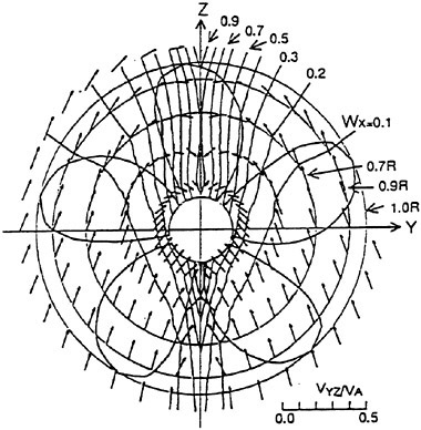
Fig. 13 Estimated wake distribution of Seiun-Maru
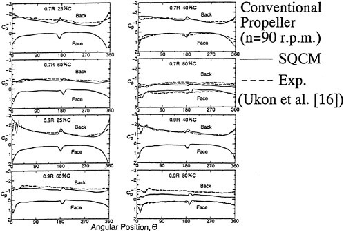
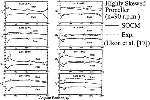
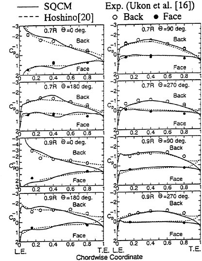
Fig. 16 Chordwise pressure distributions at 0.7R and 0.9R
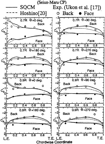
Fig. 17 Chordwise pressure distributions at 0.7R and 0.9R (Seiun-Maru HSP)
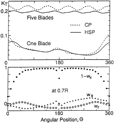
Fig. 18 Thrust fluctuation and estimated wake distributions
3.3.2 DTMB P4118
Here we compare the calculated results of the shaft forces and moments acting on the three-bladed DTMB propeller 4118 with the experimental data. The experiment was made by Boswell and Miller at DTMB [21]. Principal particulars of DTMB P4118 are shown in Table 2. The panel arrangement for the propeller is illustrated in Fig. 19. The discretizations of the blade and camber surfaces are the same as those of the Seiun-Maru CP and HSP. The harmonic wakes of 3- and 4-cycle shown in Fig. 20 are used in the experiment and the calculation.
The first examples are the shaft forces and moments in the 3-cycle wake. In Fig. 21 we can see that only the force in the X-direction and the moment around the X-axis fluctuate and other forces and moments are constant during one revolution. Fig. 22 shows the forces acting on each propeller blade in the Ζ-direction. Each force fluctuates with the angular position, but the total force of the three blades is always zero.
Next we show the shaft forces and moments in the 4-cycle wake in Fig. 23. In this case the force in the X-direction and the moment around the X-axis are constant during one revolution. Fig. 24 shows the forces acting on each propeller blade in the X-direction. Each force fluctuates with the angular position, but the total force of the three blades is always constant.
Finally we compare the calculated amplitudes of the shaft forces and moments ![]()
![]() to the experimental data. Figs. 25–27 show the comparisons between calculation and experiment. The
to the experimental data. Figs. 25–27 show the comparisons between calculation and experiment. The
agreement between calculated results experimental data is generally good.
Table 2 Principal particulars of DTMB P4118
|
DIAMETER (inch) |
12.0 |
|
NUMBER OF BLADE |
3 |
|
PITCH RATIO AT 0.7R |
1.077 |
|
EXPANDED AREA RATIO |
0.606 |
|
HUB RATIO |
0.200 |
|
SKEW ANGLE (DEG.) |
0 |
|
RAKE ANGLE (DEG.) |
0 |
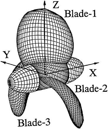
Fig. 19 Panel arrangement for DTMB P4118
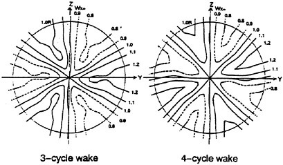
Fig. 20 Wake distributions
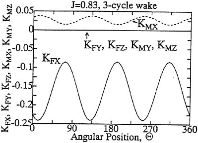
Fig. 21 Fluctuations of propeller shaft forces and moments in 3-cycle wake
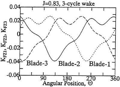
Fig. 22 Fluctuations of propeller shaft forces in 3-cycle wake
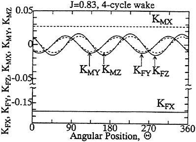
Fig. 23 Fluctuations of propeller shaft forces and moments in 4-cycle wake
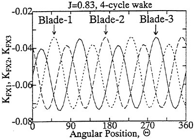
Fig. 24 Fluctuations of propeller shaft forces in 4-cycle wake
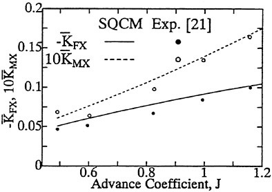
Fig. 25 Comparison of thrust and torque in 3-cycle wake

Fig. 26 Comparison of propeller shaft forces in 4-cycle wake
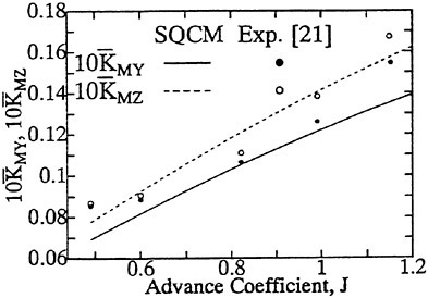
Fig. 27 Comparison of propeller shaft moments in 4-cycle wake
4. CONCLUSION
A new surface panel method “SQCM” which satisfies easily the Kutta condition was applied to Seiun-Maru CP, HSP and DTMB P4118. Comparison between the results calculated by SQCM and the experimental data led the following conclusions:
-
The Kutta condition is satisfied sufficiently in the steady problem with no iterative procedure. The typical number of iterations for the Kutta condition is about five times at each time step in the unsteady problem.
-
The calculated propeller open-water characteristics agree well with the experimental data in the steady problem.
-
SQCM can predict the blade pressure distribution and the forces accurately in the steady and unsteady problems.
ACKNOWLEDGEMENT
We wish to express our deep thanks to Mr. Daisuke Matsumoto (Graduate School, Kyushu University) for his help in completing this manuscript.
REFERENCES
[1] Hess, J.L., “The Problem of Three-Dimensional Lifting Potential Flow and Its Solution by Means of Surface Singularity Distribution”, Computer Methods in Applied Mechanics and Engineering, Vol. 4, 1974.
[2] Morino, L. and Kuo, C.-C., “Subsonic Potential Aerodynamics for Complex Configurations: A general Theory”, AIAA Journal, Vol. 12, No. 2, 1974, pp. 191–197.
[3] Koyama, K., “Flow around a Lifting Body—Flow near the Trailing Edge of a Wing—”, Text of 3rd JSPC Symposium on Flows and Forces of Ships, The Society of Naval Architects of Japan, 1989, pp. 173–201.
[4] Hess, J.L. and Smith, A.M.O, “Calculation of Nonlifting Potential Flow about Arbitrary Three Dimensional Bodies”, Journal of Ship Research, Vol. 8, No. 2, 1964, pp. 22–44.
[5] Lan, C.E., “A Quasi-Vortex-Lattice Method in Thin Wing Theory”, Journal of Aircraft, Vol. 11, No. 9, 1974, pp. 518–527.
[6] Nakatake, K., Ando, J., Kataoka, K., Yoshitake, A., “A Simple Calculation Method for Thick Wing”, Transactions of The West-Japan Society of Naval Architects, No. 88, 1994, pp. 13–21.
[7] Ando, J., Maita, S., Nakatake, K., “A Simple Surface Panel Method to Predict Steady Marine Propeller Performance”, Journal of the Society of Naval Architects of Japan, Vol. 178, 1995, pp. 61–69.
[8] Maita, S., Ando, J., Nakatake, K., “A Simple Surface Panel Method to Predict Unsteady Marine Propeller Performance”, Journal of the Society of Naval Architects of Japan, Vol. 182, 1997, pp. 71–80.
[9] Hoshino, T., “Application of Quasi-Continuous Method to Unsteady Propeller Lifting-Surface Problems”, Journal of the Society of Naval Architects of Japan, Vol. 158, 1985, pp. 48–68.
[10] Murakami, M., Kuroi, M, Ando, J., Nakatake, K., “Practical Quasi-Continuous Method to Estimate Unsteady Characteristics of Propeller”, Transactions of The West-Japan Society of Naval Architects, No. 84, 1992, pp. 23–36.
[11] Maita, S., Ando, J., Nakatake, K., “A Simple Calculation Method for Thick Wing (Continued)—Application to Thin Wing—”, Transactions of The West-Japan Society of Naval Architects, No. 92, 1996, pp. 37–44.
[12] Tanahashi, T., Mechanics of a Continuous Medium (7)—Vortex Motion and Vortex Theorem—, 1991, Rikou-Tosho
[13] Nakamura, N., “Estimation of Propeller Open-Water Characteristics Based on Quasi-Continuous Method”, Journal of the Society of Naval Architects of Japan, Vol. 157, 1985, pp. 95–107.
[14] Nakatake, K., Ando, J., Maita, S., “A Simple Surface Panel Method to Solve Unsteady Wing Problems”, Proceedings of the 7th International Symposium on Practical Design of Ships and Mobile Units, 1998, (to appear)
[15] Ukon, Y., Kurobe, Y., Kudo, T., 1989, “Measurement of Pressure Distribution on a Conventional and a Highly Skewed Propeller Model—Under Non-Cavitating Cobdition—”, Journal of the Society of Naval Architects of Japan, Vol. 165, pp. 83–94.
[16] Ukon, Y., Kudo, T., Kurobe, Y., Kamiirisa, H., Yuasa, H., Kubo, H., Itadami, Y., “Measurement of Pressure Distribution on a Full Scale Propeller—Measurement on a Conventional Propeller—”, Journal of the Society of Naval Architects of Japan, Vol. 168, 1990, pp. 65–75.
[17] Ukon, Y., Kudo, T., Kurobe, Y., Yuasa, H., Kamiirisa, H., Kubo, H., “Measurement of Pressure Distribution on a Full Scale Propeller—Measurement on a Highly Skewed Propeller—”, Journal of the Society of Naval Architects of Japan, Vol. 170, 1991, pp. 111–123.
[18] Hoshino, T., “Hydrodynamic Analysis of Propellers in Steady Flow Using a Surface Panel Method”, Journal of the Society of Naval Architects of Japan, Vol. 165, 1989, pp. 55–70.
[19] Japan Ship Research Association, “Study on Propeller and Ship Stern, Aiming at Reduction of Vibration and Noise at Ship Stern”, The Report of No. 183 Panel, No. 358, 1983
[20] Hoshino, T., “Hydrodynamic Analysis of Propellers in Unsteady Flow Using a Surface Panel Method”, Journal of the Society of Naval Architects of Japan, Vol. 174, 1993, pp. 71–87.
[21] Boswel, R.J. and Miller, M.L., “Unsteady Propeller Loading -Measurement, Correlation with Theory, and Parametric Study”, D.W.Tayler Naval Ship Research and Development Center Report 2625, 1968
DISCUSSION
Κ.Kim
Naval Surface Warfare Center, Carderock Division, USA
1. The predicted pressure distribution near the trailing edge showed a consistent difference between the SQCM and the panel method by Hoshino as shown in Figs. 9 and 10 for steady flow and in Figs. 16 and 17 for unsteady flow. Would the authors explain the difference by relating to Kutta conditions?
2. As shown in Fig. 17, the SQCM predictions of Cp are in better agreement with experimental measurements than Hoshino’s panel method at 0.7R and 0.9R and θ=90° and 270°. Would the authors explain why SQCM predictions showed better agreement than Hoshino’s panel method for the highly skewed propeller, whereas both methods predicted comparable results for the conventional propeller as shown in Fig. 16?
AUTHORS’ REPLY
We also notice the clear difference of pressure distributions between Dr. Hoshino’s result and ours. He used only 12 panels in the radial direction and 10 or 12 panels in the chordwise direction, whereas we used 20 and 30 panels, respectively. We think finer panels result in more reliable pressure distributions and the behavior of pressure near the trailing edge should resemble that of conventional wing.
As to the second discussion, we must say we cannot make it clear.
Experimental Characterization of Propeller Tip Flow
C.Chesnakas, S.Jessup (Naval Surface Warfare Center, Carderock Division, USA)
ABSTRACT
Detailed velocity measurements were made of the velocity field behind Propeller 5168 in the Carderock Division, Naval Surface Warfare (CDNSWC) 36-inch water tunnel. The measurements were made in order to examine the behavior of the tip-vortex flow. A first set of measurements was made with a three-component, non-coincident Laser Doppler Velocimeter (LDV) system at four different advance coefficients and at four downstream stations. A second set of measurements were made with a three-component, coincident LDV system at a single advance coefficient and a single downstream station. The coincident set of measurements were of higher accuracy and included data on the Reynolds shear-stress terms. Plots are presented of the detailed tip-vortex structure, and the variation of this structure with advance coefficient and location is examined. Data on the thrust, torque, and cavitation performance of the propeller are also included.
NOMENCLATURE
|
Cp |
Pressure coefficient, 1−(V/V∞)2 |
|
D |
Propeller diameter, 402.7 mm |
|
F |
Maximum blade section camber |
|
it |
Total blade rake |
|
J |
Propeller advance coefficient, U∞/nD |
|
KQ |
Torque coefficient, torque/(ρ n2D5) |
|
KT |
Thrust coefficient, thrust/(ρ n2D4) |
|
n |
Propeller rotational speed, rev/s |
|
P |
Propeller pitch |
|
p |
Static pressure in tunnel |
|
pν |
Vapor pressure of water |
|
q |
Root-mean-square (RMS) fluctuation of velocity,TKE=q2/2, normalized by U∞ |
|
r |
Radius, normalized by R |
|
R |
Propeller radius, 201.4 mm |
|
T |
Maximum blade section thickness |
|
Ur |
Radial velocity in the measured (fixed) frame, positive outward, normalized by U∞ |
|
Ut |
Tangential velocity in the measured (fixed) frame, positive counterclockwise looking downstream, normalized by U∞ |
|
Ux |
Axial velocity in the measured (fixed) frame, positive downstream, normalized by U∞ |
|
U∞ |
Inflow velocity in the stationary frame (i.e., tunnel velocity) |
|
V |
Total velocity in the rotating frame |
|
Vc |
Cross-stream velocity in the rotating frame, normalized by U∞ |
|
Vr |
Radial velocity, normalized by U∞ (identical to Ur) |
|
Vs |
Streamwise velocity in the rotating frame, normalized by U∞ |
|
Vsn |
Streamwise velocity in the rotating frame, normalized by V∞ |
|
Vt |
Tangential velocity in the rotating frame, positive counterclockwise looking downstream, normalized by U∞ |
|
Vx |
Axial velocity, normalized by U∞ (identical to Ux) |
|
Vθ |
Secondary velocity magnitude (Vc2+Vr2)1/2 |
|
V∞ |
Inflow velocity, rotating frame (U∞2+(2πrn)2)1/2 |
|
x |
Axial coordinate, from propeller mid plane |
|
η |
|
|
θ |
Circumferential angle, radians |
|
θs |
Blade skew angle |
|
ρ |
Density |
|
σi |
|
|
|
Propeller pitch angle |
|
ωs |
Streamwise vorticity, normalized by U∞/R |
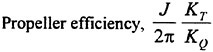
INTRODUCTION
The Naval Surface Warfare Center is presently engaged in a joint project with the Royal Netherlands Navy and Marine Research Institute, Netherlands (MARIN) to develop propeller blade tip geometries that will improve tip-vortex cavitation. The program includes development of design procedures and geometries using potential-flow
panel methods, Reynolds-Averaged Navier-Stokes (RANS) codes, and iterative propeller-model tests. To develop baseline data for a state-of-the-art combatant-type geometry, Propeller 5168 was selected for fundamental experiments to measure tip-vortex cavitation inception and near-tip velocity distributions in uniform inflow. All tests were performed in the NSWCCD 36inch water tunnel.
Measurements were first made with a hybrid lens-optic/fiber-optic LDV system which measured all three components of velocity and the normal stresses, but did not measure the shear stresses. The first set of measurements was made at several advance coefficients and at several locations downstream of the propeller. After analysis of the first data set, it was decided to make a second set of measurements using an all fiber-optic LDV system. The fiber-optic system allowed for coincident velocity measurements to be obtained, which both increased the accuracy of the mean-velocity measurements and allowed for the measurement of the shear stresses. The fiber-optic system had a much smaller effective measurement volume than the hybrid LDV system, which resulted in a lower data rate and longer data collection times. Therefore, the measurements with the fiber-optic system were obtained only at one advance coefficient and one downstream station.
The propeller, its performance, the flow about the propeller, and the instrumentation used will be described here; and the uncertainties involved in obtaining the data will be analyzed. Several plots of the data will be presented, but only at selected flow conditions. Additional treatment of the data can be found in Chesnakas and Jessup1.
EXPERIMENTAL APPARATUS
Water Tunnel
All measurements were made in the David Taylor, 36-inch, Variable Pressure Water Tunnel. The tunnel is a recirculating design with interchangeable test sections. A 36-inch diameter, open-jet test section was used for these tests. The tunnel allows the pressure in the test section to be varied so that cavitation inception can be investigated. Both upstream and downstream drives are available for propeller testing. For these tests, the propeller was driven from upstream. Inflow to the propeller was uniform except for the wakes from the three upstream shaft support struts.
Propeller
The propeller used for this investigation is the David Taylor Propeller 5168, shown in Figure 1. This is a five-bladed, controllable-pitch propeller with a design advance ratio, J, of 1.27. The propeller is left handed with a radius, D, of 402.7 mm. A cylindrical fairwater 96.8 mm long was attached aft of the propeller hub. No boundary-layer tripping was employed for these experiments. The geometry of the propeller is listed in Table 1.
Laser Doppler Velocimetry System
Two sets of LDV measurements were made with two different LDV systems. The first system was a hybrid lens-optic/fiber-optic system, and the second was an all fiber-optic system. The common elements of each system will be described in this section, while the specific elements of each systems will be described in their own sections.
Both systems utilized the blue (488 nm), green (514.5 nm), and violet (476.5 nm) beams of an argon-ion laser to measure the radial, tangential, and axial velocity components, respectively. The measurement volume was positioned at a point in the horizontal plane containing the propeller axis. The probe volumes were translated in the axial and radial directions in order to get two directions of movement in the flow field, while the rotation of the propeller relative to the measurement point provided the third direction of movement. The position of the shaft was encoded with an 8192 counts/revolution signal, which was recorded with each velocity measurement. The measurements are grouped into 1024 circumferential positions, each 8 encoder counts wide.
Doppler signals were analyzed with a TSI Model IFA 655 Digital Burst Correlator. The processor performs a 256-sample, double-clipped, autocorrelation on each doppler burst, allowing the measurement of velocity even when the signal-to-noise ratio is low. The proces-
Table 1. Propeller 5168 geometric parameters. Blade sections are non-standard.
|
r/R |
C/D |
P/D |
it/D |
|
θs (deg.) |
T/C |
F/C |
|
0.3000 |
0.20000 |
1.08750 |
0.01110 |
49.086 |
6.280 |
0.26936 |
−0.03800 |
|
0.3500 |
0.23700 |
1.24479 |
−0.00694 |
48.545 |
−0.754 |
0.17804 |
−0.00860 |
|
0.4000 |
0.27600 |
1.36525 |
−0.02370 |
47.372 |
−4.824 |
0.11423 |
0.00903 |
|
0.4500 |
0.30800 |
1.45791 |
−0.03579 |
45.882 |
−7.336 |
0.08897 |
0.01779 |
|
0.5000 |
0.33410 |
1.54131 |
−0.04367 |
44.457 |
−8.865 |
0.07546 |
0.02789 |
|
0.6000 |
0.38540 |
1.67347 |
−0.04825 |
41.599 |
−9.838 |
0.05858 |
0.03655 |
|
0.7000 |
0.43500 |
1.63334 |
−0.04195 |
36.602 |
−8.108 |
0.04874 |
0.03323 |
|
0.8000 |
0.47450 |
1.50246 |
−0.03025 |
30.871 |
−3.784 |
0.04108 |
0.02473 |
|
0.9000 |
0.46500 |
1.33483 |
−0.01645 |
25.272 |
3.784 |
0.04376 |
0.01191 |
|
0.9500 |
0.39000 |
1.18919 |
−0.00960 |
21.725 |
9.297 |
0.05883 |
0.00539 |
|
0.9800 |
0.27696 |
1.03965 |
−0.00538 |
18.659 |
13.344 |
0.06402 |
0.00196 |
|
1.0000 |
0.00000 |
0.90000 |
−0.00245 |
15.986 |
16.400 |
0.06222 |
0.00000 |
sors were operated in the random mode with the hybrid LDV system, and in the coincidence mode with the fiber-optic LDV system.
The flow was seeded with silicon-carbide powder. Since the water in the tunnel recirculates, seed needed to be added only infrequently.
Hybrid LDV System
The hybrid LDV system consisted of both a lens-optic assembly and a fiber-optic probe assembly as shown in Figure 2. The lens-optic system assembly measured two components of velocity and the fiber-optic assembly measured a single component of velocity. Each system was traversed independently.
The lens-optic assembly utilized the green (514.5 nm) and violet (476 nm) beams of an argon-ion laser to measure the tangential and axial components of velocity, respectively, in a 0.06×0.9 mm probe volume. The optics for this assembly were outside of the tunnel, and passed through a window into the water. A special insert in the open-jet test section was used to place the front lens of the assembly closer to the propeller than would normally be possible. The insert extended in the test section to just outside the open jet. This both decreased the size of the probe volume and increased the signal-to-noise ratio. The assembly was mounted on a three-component traverse.
The fiber-optic probe utilized the blue (488 nm) beam of the argon-ion laser to measure the radial component of velocity in a 0.07×1.3 mm probe volume. The fiber-optic probe was placed inside the test section, below the plane of measurements. The probe was mounted on a traverse which could be moved in both the axial and radial directions.
Because of the two separate traverses, it was difficult to keep all three measurement volumes precisely coincident. The processors were therefore operated in random mode, and Reynolds shear stress data were not acquired. Reynolds normal stresses, however, were acquired.
Fiber-Optic LDV System
The fiber-optic LDV system consisted of two TSI model 9832 fiber optic probes as shown in Figure 3. The two probes were rigidly mounted together on a traverse which could translate in the axial and radial directions. The focal distance of the probes (470 mm in water) was sufficient to place the probe bodies outside of the jet.
The horizontal probe utilized the green (514.5 nm) and violet (476 nm) beams of an argon-ion laser to measure the tangential and axial components of velocity, respectively. The vertical probe utilized the blue (488 nm) beam of the argon-ion laser to measure the radial component of velocity. Both probe volumes were 0.07×1.3 mm.
With the probes mounted rigidly together, it was possible to keep the measurement volumes precisely aligned, and the processors were operated in coincidence mode. This allowed shear stresses to be measured and velocity bias corrections to be applied to the measurements. This also reduced the effective probe volume to 0.07×0.07 mm.
TEST CONDITIONS
Velocity measurements were performed at the four advance ratios listed in Table 2. All measurements were at an approximate water temperature of 75°F. It was not possible to exactly match the flow conditions of the hybrid test when the fiber-optic test was performed. The values in parentheses at J=1.10 are for the fiber-optic LDV system, while the other values are for the hybrid system. This mismatch will be discussed further in the Results section. Tip-vortex cavitation could be observed at the two lowest advance ratios, but none was observed at the two highest advance ratios. Pressure was kept high enough during the LDV measurements to suppress cavitation, since the presence of cavitation bubbles would interfere with the propagation of the laser beams through the water.
Velocity measurements were obtained both upstream and downstream of the propeller, as detailed in Table 3. At all advance coefficients, measurements were made at an upstream location, x/R=−0.4049 as measured from the propeller mid plane, and at a downstream location, x/R=0.2386. Coincident measurements were made only at these two planes, and only for J=1.10. Non-coincident measurements were made at these two planes for four advance coefficients—J=0.98, 1.10, 1.27, and 1.52—and at additional downstream locations for J=1.10. At
Table 2. Measured flow conditions.
|
J |
n (RPM) |
U∞ (m/s) |
T (N) |
Q (N·m) |
|
0.98 |
1200 |
7.89 |
3826 |
376 |
|
1.10 |
1450 |
10.70 |
4715 (4782) |
481 (495) |
|
1.27* |
1300 |
11.08 |
2580 |
301 |
|
1.51 |
1150 |
11.73 |
667 |
122 |
|
Values in parentheses for fiber-optic system. *design condition |
||||
Table 3. LDV measurement planes.
|
|
x/R |
||||
|
J |
−0.4049 |
0.1756 |
0.2386 |
0.3963 |
0.8378 |
|
0.98 |
N |
|
Ν |
|
|
|
1.10 |
NC |
Ν |
NC |
N |
N |
|
1.27 |
N |
|
N |
|
|
|
1.52 |
N |
N |
|||
|
N—Non-coincident measurements acquired C—Coincident measurements acquired |
|||||
the downstream locations, the radial increment between measurements was 0.1R over most of the span, with a radial increment of 0.02 to 0.03R in the region of the tip vortex. At the condition of J=1.10, x/R=0.2386, measurements were spaced in a denser grid. At J=1.10, x/R=0.1756, only the tip region of the flow could be measured, due to blockage of the laser beams by the propeller.
COORDINATE SYSTEM
The measurements in the data file are all normalized by the tunnel velocity, U∞, and are presented in the rotating frame. The relation between the stationary (measured) frame velocities, U, and the rotating frame velocities, V, is:
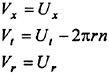
(1)
The measurements in the plots are presented in a primary/secondary coordinate system in order to highlight the vortex structure. In this coordinate system, illustrated in Figure 4, the primary velocity, Vs, is defined as being in the axial-tangential plane, at the propeller pitch angle, ![]() . The secondary velocities are then the orthogonal velocity component in the x-t plane, Vc, and the radial velocity, Vr. Since the pitch angle is different at each radius, the coordinate system is different at each radius as well. These velocity components can be calculated from:
. The secondary velocities are then the orthogonal velocity component in the x-t plane, Vc, and the radial velocity, Vr. Since the pitch angle is different at each radius, the coordinate system is different at each radius as well. These velocity components can be calculated from:
(2)
(3)
(4)
Similarly, the velocity-stress terms can be calculated from:
(5)
(6)
(7)
(8)
(9)
(10)
The secondary flow components thus defined are perpendicular to the propeller pitch line. In order to examine vectors of the secondary flow—particularly in the tip-vortex region—it is therefore useful to adjust the aspect ratio of the plot to make the vortex appear as if it were measured in a plane perpendicular to the blade pitch line. To do this, the angular coordinate for each plotted point is found from:
(11)
where θ is the actual circumferential coordinate, θp is the plotted circumferential coordinate, θc is the circumferential coordinate of the center of the plot, and ![]() is the propeller pitch angle (note that
is the propeller pitch angle (note that ![]() is a function of r). This makes the cross section of the vortex circular and makes the secondary flow vectors point in the correct direction.
is a function of r). This makes the cross section of the vortex circular and makes the secondary flow vectors point in the correct direction.
UNCERTAINTY ANALYSIS
The uncertainties for some terms are different for the hybrid LDV system and for the fiber-optic LDV system. Where the uncertainties are different for the two systems, the text will explicitly state so, and the tables will list the uncertainty for the hybrid system normally, with the uncertainty for the fiber-optic system following italicized in parentheses.
Elemental Uncertainties
The uncertainties for the fundamental quantities measured in this experiment are listed in Table 4. Those uncertainties which are the same for all measurements are listed as bias uncertainties, and those uncertainties which vary for each measurement (and thus can be reduced by statistical averaging) are listed as precision uncertainties. Uncertainties are listed as a fraction of the nominal value, unless otherwise noted.
The uncertainties in x, t, and r are the uncertainties in positioning the probe volume with respect to the propeller. The Δx, Δt, and Δr uncertainties are the uncertainties in positioning the three probe volumes with respect to each other. Since coincidence between the probe volumes is ensured by the coincidence mode of the processor, this uncertainty is zero for the fiber-optic system. Uncertainty in the measurement of the frequency is assumed to be small relative to the uncertainty due to finite sample size, and so is ignored. The uncertainty in the perpendicularity of the three measured components is assumed to be small compared to the uncertainty in fringe spacing and probe volume coincidence, and is ignored as well.
Calculated Uncertainties
The calculated uncertainties for the quantities found by combining other measurements are presented in Table 5. The calculation of the uncertainty in J from the uncertainties in Table 4 is straight forward. However, the rest of the items in Table 5 can only be calculated with information on the local flow conditions. This is because
Table 4. Elemental Uncertainties
all of these items depend on the values of the velocity, velocity gradients, or turbulence intensity. The uncertainties in Table 5 are therefore listed for two representative flow conditions. The first, case 1, is a point in the “inviscid” flow between the blade wakes. In this region, the turbulence intensity is low and the flow gradients are small. Case 1 is representative of the majority of the flow. For case 1, the benefits of operating the LDV system in coincidence mode are minimal, and the uncertainties in this region are essentially the same for the hybrid and all fiber-optic measurements. Case 2, is a point in the tip vortex. At this location the turbulence intensity and the velocity gradients are at their highest values, and so the uncertainties are a maximum. Case 2 is representative of only a very small fraction of the flow, but the fraction of most interest. For case 2 the severe flow gradients make precise alignment of the measurement volumes essential, and the accuracy of the hybrid system suffers as a result.
For case 1, the velocity uncertainties are all below 0.5% of the inflow velocity. In this region of the flow, the velocity uncertainty is dominated by the uncertainty in the fringe spacing of 0.3%. Flow gradients in this region are small, so the uncertainties for the two LDV systems are identical.
For case 2, the uncertainties are higher due to a number of effects. The precision uncertainty is higher than in case 1 due to the uncertainty in finding the mean in a high turbulence region with a relatively small sample size (~250). The bias uncertainty is higher due to two effects. First, the high turbulence intensity causes there to be a bias in the average velocity towards fluid traveling with a higher total velocity, due to the correlation between particle arrival rate and fluid velocity. In a highly three-dimensional flow, this can be corrected using knowledge of the correlation between the different velocity compo
Table 5. Calculated Uncertainties.
|
|
Case 1 (Inviscid Flow) |
|
||
|
Item |
Bias |
Precision |
Total |
Reference |
|
J |
0.005 |
0.003 |
0.006 |
J |
|
Ux, Vx |
0.003 |
0.002 |
0.004 |
U∞ |
|
Ut |
0.001 |
0.001 |
0.002 |
U∞ |
|
Ur, Vr |
0.0003 |
0.001 |
0.001 |
U∞ |
|
Vt |
0.001 |
0.001 |
0.002 |
U∞ |
|
Vs |
0.002 |
0.002 |
0.003 |
U∞ |
|
Vc |
0.003 |
0.002 |
0.004 |
U∞ |
|
Vν |
0.003 |
0.002 |
0.004 |
U∞ |
|
q |
0.00 |
0.10 |
0.10 |
q |
|
VxVt… |
0.0000 |
0.0001 |
0.0001 |
U∞2 |
|
VsVc… |
0.0001 |
0.0001 |
0.00015 |
U∞2 |
nents, so this adds uncertainty only to the measurements with the hybrid LDV system. Second, the high gradients in velocity combine with the uncertainty in probe-volume coincidence to give a bias uncertainty in velocity. This is the dominant source of velocity uncertainty for the hybrid system. It is not present for Vt, since it is assumed that the measurement volume for that component is the probe position, and errors in probe volume coincidence are relative to that volume.
Precision uncertainty in the measurement of the turbulent velocity fluctuations, q, is dominated by the uncertainty in finding the variance of a distribution with a finite sample size. For a sample size of 250, that uncertainty is approximately 10%. Bias in the turbulence intensity measurements arises due to non-coincidence of the probe volumes, and so is only present for the hybrid measurements. It should be noted, however, that the LDV has a lower noise floor, below which it can not measure the turbulence. For this setup, the noise floor in q was approximately 1.5% of the measured velocity
Uncertainties for the Reynolds shear stress terms apply only to the fiber-optic measurements, since only those measurements yielded the shear stress terms. The row labeled VxVt contains the uncertainties for the measured shear stress terms, while the row labeled VsVc contains the uncertainties for the transformed shear stress terms. The precision uncertainty for these terms comes from the statistical uncertainty resulting from the relatively small sample size. Bias in the measured terms is small, but some bias is introduced to the transformed terms due to the inability of the system to measure a zero normal stress.
Uncertainty in the magnitude of the streamwise vorticity was difficult to estimate analytically. The effect of velocity bias on the streamwise vorticity was estimated by multiplying the measured velocities by (1+q2/U2)−1, where U is the velocity magnitude in the fixed (measured) frame, and recalculating the vorticity. The change in streamwise vorticity was on the order of only 3%. The effect of other sources of uncertainty was quantified by analyzing variations in vorticity between differing blades and between different measurement sets. The numbers found from this analysis were much higher than 3%, and are listed in Table 5. Uncertainty for the hybrid system is much higher than for the fiber-optic system due to the possible misalignment of the probe volumes. No uncertainty is listed for case 1 (the inviscid region) since ω is near zero in this region.
Uncertainty in the inception cavitation number was primarily a precision uncertainty. From the inception data scatter over all the measurements taken, uncertainty in σi was estimated as ±0.4.
Assessment of Model Propeller Geometry
Model Propeller 5168 was manufactured using numerical control milling techniques, representing state-of-the-art model manufacturing. To assess the accuracy of the model, each of the five blades was measured at r=0.32, 0.34, 0.5, 0.7, 0.9, 0.95, 0.97, and 0.98. Comparison of the measurements to the design geometry showed some deviation near the tip, where the leading edge was “cut back” relative to the design offsets, and a slight pitch deviation over most of the blade.
An attempt was made to quantify the effects of the deviations documented in the geometry measurements. Calculations were performed with the panel code with estimated geometry deviation. The deviations changed the minimum pressure coefficient, Cp, at the blade tip as much as 0.2. This was about half the estimated error in the measurement of the tip-vortex cavitation inception number. It should be acknowledged that the panel code is not capable of accurately calculating the Cp associated with tip-vortex inception, but it may be capable of predicting relative values when perturbing geometry.
RESULTS
Propeller Performance
Initially, propeller 5168 was operated at high tunnel pressure to suppress cavitation and run at 9.84 m/s over a range of J to determine the thrust and torque “open-water” performance. The propeller had been open-water tested earlier in the NSWCCD towing basin. Figure 5 shows good comparison of the basin result and the measurements in the 36-inch water tunnel, thus validating the open flow characteristics of the open jet test section of the 36-inch water tunnel.
Cavitation Performance
Fundamental cavitation inception tests were performed in the 36-inch water tunnel. The propeller was driven from upstream and run over a range of speeds and advance coefficients to identify the inception of suction and pressure-side tip-vortex cavitation.
Cavitation Inception
During cavitation tests, air content was maintained within a range of 60–80%, as has been the standard procedure for the 36-inch water tunnel at NSWCCD. Cavitation inception was determined by initially operating the propeller at a condition of no cavitation, then increasing propeller rpm until tip-vortex cavitation occurred. Inception was noted when three of the five blades showed intermittent tip-cavitation events at a rate of one event in ten seconds when observed with strobe illumination. Blade Reynolds number at inception, based on chord length at r=0.7 of 0.870R, ranged from 3.2 to 5.7×10⁶.
Figure 6 shows the tip-vortex cavitation inception results. Typical behavior is seen for suction-side and pressure-side tip-vortex cavitation. Suction-side cavitation was observed relatively far downstream, approximately one-half rotation of the blade, at high loading (low J). At low loading (J>1.1) the inception was observed closer to the blade, typically within 50 mm of the tip. Slight differences were seen at the two static pressures at which suction side tip-vortex cavitation was observed. The Reynolds number is about 10% lower at the lower pressure, and the lower σi observed at the lower speeds and static pressures is qualitatively consistent with Reynolds number scaling.
Pressure-side tip-vortex cavitation was observed emanating from pressure-side leading-edge cavitation. No coherent pressure-side vortex structure was observed. At CDNSWC, any pressure-side cavitation seen outboard of the 0.95 radius is normally categorized as pressure-side tip-vortex cavitation
Attachment Point and Trajectory
Over the range of J tested, suction-side tip-vortex attachment occurred aft of the blade tip. The attachment location was determined by reducing pressure until the tip vortex was persistent enough to, at least intermittently,
attach to the blade. The average location at J=0.98 was the blade trailing edge at 0.997 radius, while at J=1.1, the attachment point moved aft to 0.998 radius trailing edge.
The pitch angle and radial location of the cavitating tip vortex was also observed. Using a sighting telescope attached to an angular measurement device, the pitch angle of the cavitating vortex was tracked from the blade tip to an axial location of approximately one diameter downstream. The radial location of the vortex was tracked using the LDV beam crossing point and the LDV traverse. Figure 7 shows the result of these measurements. The maximum tip-vortex pitch occurred at x/R=0.4, with the pitch and radius becoming constant downstream of x/R=1.6.
Circumferentially Averaged Velocities
The measured circumferentially averaged velocities at x/R=0.2386 at varying J are shown in Figure 8. This figure shows that as loading increases (J decreases), the magnitude of all velocity components increases. At the tip, all Ux approaches 1 and Ut and Ur approach zero, although Ur approaches slowly.
A comparison between the measurements made with the hybrid system and measurements made with the fiber-optic system shows that the circumferential averages do not precisely match. For the hybrid system the axial and radial velocities are about 0.03 and 0.02U∞ smaller, respectively, than for the fiber-optic system for r>0.5. The tangential velocity for the hybrid system is slightly smaller (up to 0.006U∞) for r<0.7 and slightly larger (up to 0.006U∞) for r>0.7. As was noted in the Test Conditions section, it was not possible to precisely match the torque and thrust of the earlier set of measurements when the fiber-optic measurements were taken. Thrust was 1.4% higher for the fiber-optic measurements, and torque was 2.8% higher. This is consistent with the measured velocity differences.
Measurements were made of the velocity at x/R=1.091 across the propeller diameter using a long-focal-length, lens-optic LDV system. These measurements show that there is a slight asymmetry in the flow with the window present. Axial velocity matches well on both sides of the tunnel centerline, but tangential velocity is slightly lower on the side away from the window insert than near it. It is believed that the discrepancy in flow conditions between the two sets of measurements is due to the window insert which was present for the hybrid measurements and not present for the fiber-optic measurements. Unfortunately, it was not possible to make similar measurements across the diameter of the propeller without the insert present. Whatever the cause of the differing flow conditions for the hybrid and fiber-optic measurements, it should be noted that the measurement sets are at slightly different conditions.
Mean Velocity
In this section, plots will be shown of the flow structure downstream of the propeller blade. Measurements were made of all five blades, but it is only possible here to show the results for a single blade. The reader should note, though, that small differences do exist between the blades, as is detailed in the Blade-to-Blade Variation section.
Figure 9 shows the tip vortex behind blade 3 at x/R=0.2386, J=1.10 with secondary flow vectors plotted on top of contours of the streamwise velocity. In this figure, the aspect ratio of the plots has been adjusted as explained in the Coordinate System section. There is a deficit in velocity at the vortex core, and at this downstream location there is still a strong interaction between the tip vortex and the blade wake. This can be better seen in Figure 10, which shows the contours of the secondary velocity magnitude, Vθ, at the same conditions. The secondary velocity about the vortex is much stronger on the side opposite the blade wake than on the side next to the wake. This demonstrates the strongly asymmetric structure of the vortex.
The interaction between the wake and the tip vortex decreases as the flow moves downstream. This can be seen in Figure 11, a composite figure of all the measured downstream planes for J=1.10. In this figure, the contours again show the magnitude of Vs/V∞, For clarity, one blade has been removed from the figure, and a streamtube has been drawn to visually connect the measured vortex cores. The lines in the figure are the secondary-flow streamlines, which show the circulation of the flow around the tip vortex, and a very low energy recirculation of the flow in the middle of blade passage. This figure clearly shows the rapid decay and stretching of the wake and the separation of the wake from the vortex as the flow moves downstream. (Note that the slight lumpiness in the wake at x/R=0.239 is an artifact of the interpolation required to generate the contours in regions where the grid aspect ratio is very large and is not representative of the actual flow.)
Turbulence
Figure 12 shows plots of the rms turbulence, q, in the tip-vortex region as the flow moves downstream for J=1.10. The figure shows that, although the region of high turbulence around the vortex becomes larger as the flow moves downstream, the peak value of turbulence in the vortex does not change. The tip vortex is very strongly entangled with the blade wake at x/R=0.1756, and still is at x/R=0.3693. Only at the last measurement station, x/R=0.8378, is the tip-vortex independent of the wake flow.
The lobes of turbulence at the vortex core shown in Figure 12, x/R=0.2386 and 0.8378, appear to be an artifact of the measurements rather than a part of the flow. The non-coincidence of the three probe volumes results
in the peaks in the three turbulence components not occurring in the same location.
Figure 13 shows contours of the ![]() shear stress behind blade 3. In this figure, two cuts through the vortex have been made—one in the radial direction and one in the circumferential direction, and the flow conditions along these cuts are also shown in the figure. The RMS turbulence in the radial cut shows a double peak, while in the circumferential cut shows a single peak. It is not clear if this reflects an actual minimum in turbulence near the vortex core or some measurement bias. The secondary velocity, Vθ, is substantially smaller on the side of the vortex towards the wake, reflecting the wake/vortex interaction. The dominant shear stress in the vortex region is
shear stress behind blade 3. In this figure, two cuts through the vortex have been made—one in the radial direction and one in the circumferential direction, and the flow conditions along these cuts are also shown in the figure. The RMS turbulence in the radial cut shows a double peak, while in the circumferential cut shows a single peak. It is not clear if this reflects an actual minimum in turbulence near the vortex core or some measurement bias. The secondary velocity, Vθ, is substantially smaller on the side of the vortex towards the wake, reflecting the wake/vortex interaction. The dominant shear stress in the vortex region is ![]() which is what would be expected for an isolated vortex with minimal streamwise-velocity gradients.
which is what would be expected for an isolated vortex with minimal streamwise-velocity gradients.
Streamwise Vorticity
The streamwise vorticity was calculated as that component of the vorticity in the direction of Vs as defined earlier. In the s-c-r coordinate system (streamwise, cross-stream, radial), the streamwise vorticity is calculated from:
(12)
The measurements are, however, not in the c-r plane, but rather in the t-r plane. To evaluate the cross-stream derivative, the substitution
(13)
is used. The results of these calculations are shown in Figure 14.
Figure 14 shows the streamwise vorticity for the four measured advance coefficients at x/R=0.2386. The tip vortices for this prop spin in the counter-clockwise direction, looking downstream, and so the vorticity in the tip regions is negative. In Figure 14, the large decrease in tip streamwise vorticity is seen with increasing J. At J=0.98, the peak vorticity is approximately −375 U∞/R, at J=1.10, that value is down to approximately −200, and at J=1.52, the tip vorticity has disappeared.
The strength of the vortex, as revealed by the measurements of streamwise vorticity, remains intact as the flow moves downstream. At J=1.10 four downstream planes were measured. The peak vorticity in the four locations varies from about −225 to −170 U∞/R. The variation of streamwise vorticity is not monotonic with x, and is therefore believed to be due to the uncertainties in the calculation of ωs, and not representative of changes in the actual vortex strength.
Variations in the Measurements
Blade-to-Blade Variation
The structure of the vortex and the velocity deficit in the core is nearly identical for the different blades. The position of the core, however, varies slightly from blade to blade—presumably due to slight variations in blade geometry. The vorticity in the core of the vortex also varies. Peak vorticity—as measured at J=1.10, x/R=0.2386 with the fiber-optic system—varies from −420 U∞/R for blade 4 to −590 U∞/R for blade 5. It is believed that this variation is not a measurement artifact, since there are clearly differences in the cavitation inception among the blades and nearly identical variation is seen in the measurements made with the hybrid system. It is therefore recommended that any comparisons of the data to calculated flowfields should take these variations into account. Comparisons of the tip vortex should be performed only after the core positions have been aligned, and comparisons to the measured flow should be made for multiple blades, not just a single blade.
Measurement Set Variation
There is also some difference between measurements made with the two LDV systems. As was previously noted in the Test Conditions and Circumferentially Averaged Velocities sections, the flow conditions measured by the two systems did not match exactly, presumably due the effect of the window insert used with the hybrid system. Some of the differences between the two data sets is likely due to this slight variation in flow conditions, but the majority of the difference appears to be due to the relatively poor alignment of the probe volumes with the hybrid system. As detailed in the Uncertainty Analysis section, this causes the accuracy of the hybrid-system measurements to be significantly reduced in the tip-vortex region.
The differences are seen in the magnitudes of all the measured quantities in the core. The differences in the magnitude of the measurements correspond to the uncertainties listed in Table 5. The quantity most effected then, is the streamwise vorticity, which is found to be about half the value at the core with the hybrid system as with the fiber-optic. The shape of the contours in the vicinity of the tip vortex are also effected. The misalignment of the probe volumes causes a certain lumpiness in some of the plots, as was shown in Figure 12. These differences are more thoroughly covered in Chesnakas and Jessup1.
There does appear to be consistency in the hybrid vorticity measurements, however. Blade-to-blade variations match well for both systems. Comparisons between different conditions measured with the hybrid system should therefore be valid, although the levels may be displaced.
Comparison of Measurements to Flow Models
Some comparisons of the measured results to flow models are useful to verify measured results and validate aspects of flow modeling. Calculations of Propeller 5168 performance in uniform inflow were made with the potential based panel method, PSF102. The method calculates the blade pressure distribution, spanwise loading, and overall propeller thrust and torque. From the measured circumferential-average tangential velocity, the blade spanwise circulation can be derived3. Comparison of the measured circulation at the x/R=0.2386 plane and the calculated blade circulation in Figure 15 shows a close match over the mid-span region. Near the tip, a significant deviation occurs due to the vortex formation and contraction. At the lowest loading condition of J=1.52, negative circulation is seen, which corresponds to a weak secondary vortex, which is shown in Figure 14.
From the measured result, the pitch of the wake can be determined and compared to the wake model used in PSF10. The measured wake pitch is determined from:
(14)
The pitch of the blade wake is determined by averaging the flow pitch on either side of the blade viscous wake. This is compared to the geometric pitch and the pitch used in the PSF10 calculation, which is based on the model in the lifting surface code, PSF24. Figure 16 shows that there is a reasonable comparison over the midspan of the blade with the lifting surface model. The geometric pitch clearly underestimates the measured result. Also shown is the pitch of the vortex core, which was determined by tracking the noncavitating vortex core at the three near propeller downstream planes. It should be noted that the ultimate wake tip-vortex pitch derived using PSF2 has a value of 1.42, which compares well with the value shown of 1.43. Unfortunately, there is a discrepancy with the visually sighted cavitating tip-vortex pitch shown in Figure 7, with a far wake value of 1.48, and near wake values as high as 1.6.
CONCLUSIONS
The work here presents perhaps the most detailed published measurements of a propeller tip vortex to date. All velocity components have been resolved in the rotating frame of the propeller with sufficient spatial resolution to reveal many details of the tip-vortex flow. These measurements were made at four different advance coefficients and, at the primary advance coefficient of 1.10, at four different downstream planes. In addition, the full Reynolds-stress tensor was measured in one plane for the primary advance coefficient. These measurements will be useful not only as a numerical test case, but also as a guide to better understanding the physics of tip-vortex flows.
The measurements were performed with two different LDV systems. The hybrid LDV system measured only the mean velocities and the normal stresses. The fiber-optic system measured the shear stresses as well. The uncertainty analysis shows that, for most of the flow, the both systems measure the flowfield with excellent accuracy. However, very near the tip vortex, the high turbulence intensities and high velocity gradients reveal the limitations of the hybrid system. The inability to precisely align the three measurement volumes in the hybrid system makes the measurements of lower accuracy in the tip-vortex region. This is reflected most in the measurements of streamwise vorticity; the hybrid system measurements of ωs are consistently lower than the measurements made with the fiber-optic system.
Although every attempt was made to match the measurements made with the fiber-optic LDV system to those made with the hybrid system, the two sets were made at slightly different flow conditions. It appears that the window insert used with the hybrid system caused a small flow asymmetry which made matching the flow conditions impossible.
Strong asymmetry in the tip vortex was observed due to interaction with the wake. This asymmetry decreased as the flow moved downstream and the vortex separated from the wake.
Vortex strength varied strongly with advance coefficient. Though quite distinct at J=0.98 and 1.10, the tip vortex was very weak at the design J of 1.27, and at J=1.52, the tip vortex was virtually non-existent. In cavitation inception tests, no tip cavitation was observed at the two highest advance coefficients.
Small but significant differences were observed in vortex strength and position from blade to blade. The blade-to-blade variation was consistent with both LDV systems. Any comparisons of this data to calculations of the tip vortex should take into account this variation. Vortex cores should be aligned before making direct comparisons, and calculated quantities should be compared to the range of measurements.
ACKNOWLEDGEMENTS
This work was sponsored by the Office of Naval Research, performed by the Carderock Division of the Naval Surface Warfare Center, Code 5400 under the 6.2 Surface Ship Technology Program.
REFERENCES
1. Chesnakas, C.J., and Jessup, S.D., “3-D LDV measurements of the Flow Around Propeller 5168,” CDRKNSWC/HD-1460–02, May 1998, Naval Surface Warfare Center, Carderock Division, West Bethesda, Maryland.
2. Kerwin, J.E., et. al., “A Surface Panel Method for the Hydrodynamic Analysis of Ducted Propellers,” Transactions SNAME, Vol. 95, 1987.
3. Kerwin, J.E., “Flow Field Computations for Noncavitating and Cavitating Propellers,” 14th Symposium on Naval Hydrodynamics, Ann Arbor, Michigan, 1983.
4. Greeley, D.S. and Kerwin, J.E., “Numerical Methods for Propeller Design and Analysis in Steady Flow,” Transactions SNAME, Vol. 90, 1982.
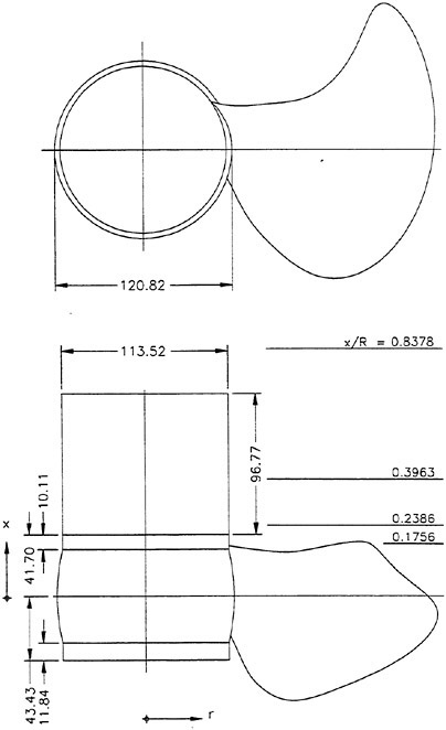
Figure 1. Propeller 5168, with fairwater and LDV measurement planes. Only 1 blade of 5 shown. Dimensions in millimeters.
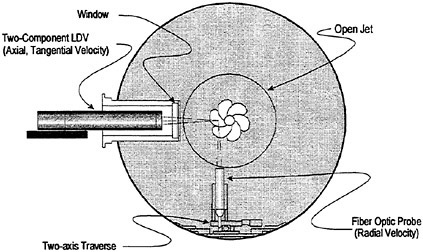
Figure 2. Hybrid lens-optic/fiber-optic LDV system in the 36-inch water tunnel.
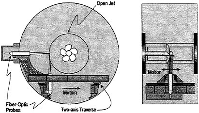
Figure 3. All fiber-optic LDV system in the 36-inch water tunnel.
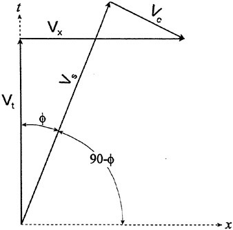
Figure 4. The secondary-flow coordinate system.
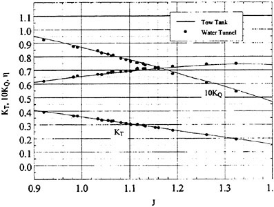
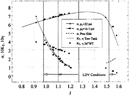
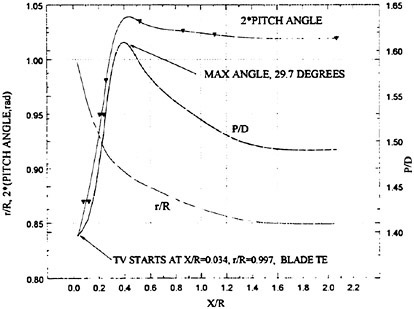
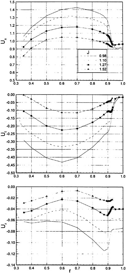
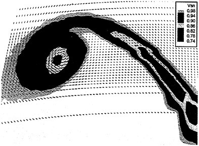
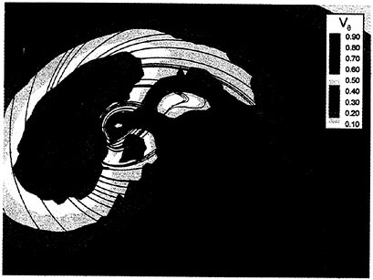
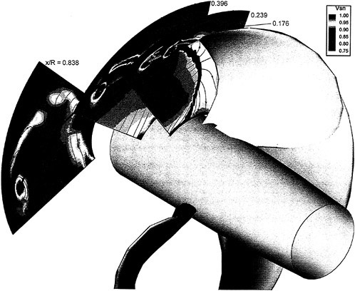
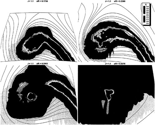
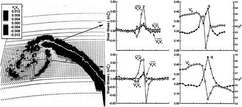
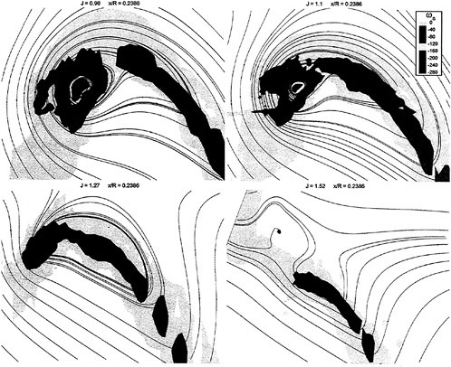
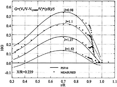
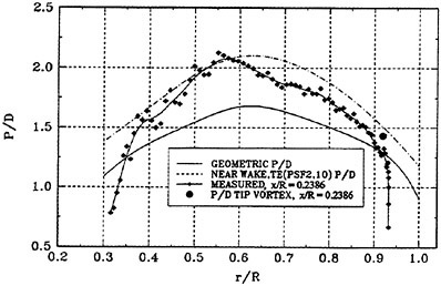
DISCUSSION
D.Fruman
Ecole Navale, France
I have to congratulate the authors for the very careful measurements they have conducted. My question refers to the effect of the measuring volume and the wandering on the measured mean velocities and velocity fluctuations in the core region where the velocity gradient and the velocity curvature are very large. Have the authors made any correction to their measurements to account for this effect?
AUTHORS’ REPLY
We believe that the fluctuations in the core trajectory are quite small at the measurement positions presented here. Visually, when the propeller is observed under strobe illumination, the position of the cavitation trail is quite steady to at least one propeller diameter downstream. Also, on another propeller of quite similar blade shape, we performed measurements of the tip-vortex flowfield with the small probe volume used here, and with a probe volume several times larger. We saw no difference in the measured flowfield; therefore, we believe no correction is necessary.
DISCUSSION
U.Bulgarelli
Istituto Nazionale per Studi ed Esperienze di Architettura Navale, Italy
When the blade-to-blade variation is less than the confidence interval, is the flow the same? In other words, can you recognize the difference, if there is one, in order to validate a CFD code?
AUTHORS’ REPLY
There clearly are blade-to-blade variations for this propeller. Although this is not clear in all measured quantities (the core velocity deficit, for example, varies only slightly), there are other quantities (such as core position) which show variations which are well outside of the measurement uncertainty. These flow variations result from small differences in the blade shapes.
When comparing these measurements to calculations for the purpose of code validation, we recommend using a validation level which sums not only the code uncertainty and the listed measurement uncertainty, but which also sums the blade-to-blade variation. This last term could be called a geometry uncertainty.
Propeller Wake Evolution Analysis by LDV
A.Stella, G.Guj (Università di Roma Tre, Italy),
F.Di Felice (Istituto Nazionale per Studi ed Esperienze di Architettura Navale, Italy), M.Elefante (Italian Navy Cavitation Tunnel, Italy)
ABSTRACT
A propeller wake investigation is carried out using LDV in a cavitation tunnel. The analysis is focused on the geometrical and hydrodynamic features of downstream wake evolution because the model arrangement in the test section enables slipstream to evolve freely for many diameters. The viscous blade wake, originated by the boundary layer on the blade surfaces, the trailing vortex sheets, due to the radial gradient of the bound circulation, as well as the turbulence distribution are resolved in the trailing edge flow and discussed. The near wake geometry is characterised by marked deformation processes, due to the bending of the blade wake sheets, the contraction of the slipstream and the trajectory of the tip vortex. Furthermore, the turbulent diffusion and the viscous dissipation lead rapidly to marked broadening and decay of the trailing edge wake. The roll-up and viscous effects in the spiraling process are also pointed out. Finally, the slipstream instability and the breakdown of the hub and tip vortices system are outlined also by means of flow visualizations.
1. INTRODUCTION
The accurate experimental wake investigation of a propeller holds an important role in the design and the performance analysis of such propulsion systems. Wake survey represents indeed a means to both locally check the fulfillment of design requirements, for instance by using the deduced blade sections drag coefficients and bound circulation distribution (1),(2), as well as to get preliminary information for new propeller design. In modern design trend the complexity of blades geometry is increasing, aiming to reduce noise generation, propeller-induced hull ship vibrations, as well as efficiency decay due to cavitation. This aspect has implied a rising interest on detailed measurements of the propeller flow field, in order to have a better knowledge of the flow details, particularly for the effects of viscosity and turbulence.
Flow velocity measurements are also important for the validation of existing propeller codes. Most current numerical methods for propeller analysis are based upon potential flow representations and simplified wake models. Nevertheless, a detailed representation of the viscous aspects (1),(3), the hub effects (4) and the actual wake-induced velocity field (5),(6) is required to enhance the accuracy of numerical predictions. The availability of reliable and detailed experimental measurements will contribute to fulfil this goal, providing both guidelines for the development as well as the validation of future theories and numerical codes.
Laser Doppler Velocimetry (LDV) was widely used in the past to measure propeller wake flow field (1),(2),(7),(8),(9) et al., which is characterized by marked velocity gradients and high turbulence levels. LDV is actually an adequate measurement technique to investigate a such complex flow, particularly for the non-intrusive probe and velocity direction recognition, along with its high spatial resolution and good frequency response.
1.1 Research Goals
In the available literature concerning the experimental investigation by LDV of the flow field around propellers, works specifically aimed to survey the downstream evolution features of the wake are rare. Guidelines on this objective have been provided by Min (7), Cenedese (8) and Hoshino (9).
A suitable experimental facility is a basic requirement in order to carry out accurate investigation of the propeller slipstream. Test conditions including the model driven from downstream or a test section relatively short with respect to the propeller diameter, are adequate for the analysis of the blade flow. Nevertheless, such conditions do not allow to work out wake evolution analysis because slipstream is obstructed from freely develop. The characteristics of the wake of a propeller model, tested in an hydrodynamic tunnel, can be indeed significantly different from those occurring in a real operative condition, as an effect of the model arrangement and the test section features.
In the present study, these problems are overcame since the model is mounted on a front
dynamometer shaft, the test section length is almost 10 times propeller diameter and the blockage ratio is about 10%. Thus, wake downstream evolution is undisturbed as in a real operative condition.
In view of the advantages given by the experimental facility, the goal of the present research is primarily the analysis of the propeller wake evolution from the trailing edge to the first diameter downstream. Furthermore, the instability of slipstream and the consequent breakdown of the hub and tip vortices system are outlined.
Wake analysis is developed considering three regions in the flow field behind the propeller: the trailing edge wake, the near wake (within the first diameter) and the far wake (up to wake breakdown).
The LDV measurement map is limited within the near wake, because flow visualizations point out that the amplitude of unsteady spatial fluctuations of the propeller slipstream are too large farther downstream. Flow visualizations in incipient cavitation conditions are used to explain and compare LDV measurement results, as well as to investigate the near and the far wake.
Although wake details are strictly dependent on both the geometry of propeller and the loading conditions, results of this investigation will be discussed with emphasis on those flow features or processes of a general content.
2. EXPERIMENTAL SET-UP
2.1 Experimental facilities
The LDV measurements and the visualizations of the wake were performed at the Italian Navy cavitation tunnel (C.E.I.M.M.), which is sketched in figure 1. The test section is square, closed jet type, 0.6 m ×0.6 m×2.6 m. Perspex windows on the four walls enable optical access. The nozzle contraction ratio is 5.96:1 and the maximum water speed is 12 m/s. The maximum free stream turbulence intensity in the test section is 2% and reduces to 0.6 % in the propeller blade inflow at 0.7 r/R, in the adopted test conditions. The flow uniformity is within 1% for the axial component and 3% for the vertical one.
The four blades propeller model (figure 2) is skewed, with a uniform pitch (pitch/diameter=1.1) and with a forward rake angle of 4° 3”.
The sketch of the instrumentation set-up is shown in figure 3. A 5 mW He-Ne, two channels, reference beam, forward scatter LDV system with trackers was used. The optics were arranged to measure two orthogonal components of velocity simultaneously (V1,V2). Both beam separation and frequency shift are provided by a rotating diffraction grating. The trackers supply two TTL signals (DO1, DO2) to detect the presence of Doppler-bursts. The measurement volume dimensions with the adopted optical configuration are 0.14 mm×5.3 mm. The probe volume can be traversed in the test section with an accuracy of about 0.01 mm. The initial reference position was fixed with an accuracy of about 0.1 mm by using a special target device. The tunnel water was initially filtered, and then seeded with 4 μm, spherical particles with high diffraction index. During the measurement campaign the Doppler signal presence percentage remained within 5÷20% at the water speed of 5 m/s. A rotary incremental encoder supplies the actual propeller position with an angular resolution of 0.1°. The encoder signals are processed by a special instrument, which provides propeller position information in different codification (analog, digital, trigger signals). Data acquisition is accomplished using a PC. An A/D converter, programmable board and a programmable input/output card were attached to PC as data interfaces. The A/D board resolution is 12 bit, corresponding to a velocity resolution of 2 cm/s.
2.2 Co-ordinate Systems
A Cartesian O-x,y,z and a cylindrical coordinate system Ο-x,r,φ (figure 4) were considered. The LDV system was arranged to measure simultaneously the axial and vertical components of the velocity in the test section fixed frame. In view of the axial symmetry of the propeller inflow and the steady conditions of operation, when the measurement volume is located on the vertical radius (along z-axis), the axial component of the velocity and the vertical one correspond respectively to the axial and the radial components in the propeller moving frame. When the probe is instead located in the horizontal radius (y-axis), they represent the axial and the tangential components of the velocity.
2.3 Measurement Map and Test Conditions
In the propeller blade reference frame, all the measurements in a circumference can be accomplished without moving the LDV volume. So the map of measurement points in a plane is obtained by only radial movements of the probe. The presence of the hub and model support, which denies optical access to laser beams, does not allow measurements of the tangential component in the region between the blade trailing edge and the hub tip.
The map of the measurement points to study the near wake is shown in figure 5. The first of five measurement disks is located as near as possible to the blade trailing edge line. The distance of 2.15R for the last one was selected referring to wake visualizations accomplished before the LDV measurements campaign, which showed the unsteady wake vortex system oscillations become too large farther downstream. In fact, flow visualizations prove that from about one diameter behind propeller the amplitude of the tip vortex spatial fluctuations becomes comparable with its
transversal dimension. The consequent, relative displacement between this oscillating coherent structure and the LDV measurement volume, which is fixed in the test section frame of reference, does not allow to characterize the velocity field of the tip vortex, using such local measurement technique. Instantaneous descriptions of the cross velocity field in the wake should be required in order to separately resolve the spatial oscillations of the coherent structures and their peculiar velocity field.
The LDV measurements were carried out with the propeller angular velocity of 25 rps and the water speed of 5 m/s, corresponding to an advance ratio J=V∞/(nD) of 0.88, near the design value. The blade Reynolds number is equal to 1.2·106 at 0.7 r/R and the cavitation number is 10.5, referred to the inflow velocity V∞. Different test conditions were adopted for the flow visualizations and will be specified for each presented result.
2.4 Phase Sampling
Measurements were worked out in poorly seeded water conditions, as required in a cavitation tunnel in order to accurately test propeller cavitation performances. Nevertheless, this test condition is unsuitable to obtain high data rates when measurements are performed using LDV. In order to efficiently acquire the remarkable amount of LDV data needed for an accurate and spatially detailed wake analysis, an efficient phase sampling technique was implemented. The tracking triggering technique TTT foresees the acquisition of the velocity sample, V1 or V2, when Doppler signal is detected on the corresponding LDV system channel. The velocity sample is tagged with the actual propeller position at the measurement time. This process is repeated independently in the two LDV channels, because it was experienced that Doppler burst detection is not necessarily simultaneous. The sequence of samples provided by the TTT at a fixed radius and a certain axial cross plane, is arranged inside angular slots of width ε. A certain velocity sample Vi[φ(t*)], acquired when the angular position was φ(t*), is put in the slot whose center is φK, if:
(1)
The slot width ε is chosen looking at two opposite considerations: angular resolution in the wake measurements improves with increasing the number of slots, but, on the other side, the greater is the number of slots, the lower is the confidence interval of statistical calculations inside a slot. In the present research an angular resolution of 2° is adopted.
A second phase sampling technique, the angular triggering technique ATT, was implemented basing upon an angular triggering approach. This technique enables both to control the angular position of the LDV measurement as well as a high accuracy of results, particularly where flow fluctuations are the highest. In view of its features, the ATT was used to deepen the analysis of the turbulent wake, through the calculation of the Reynolds stresses. In the ATT the LDV sample is acquired when propeller reaches the selected triggering angular position. In order to increase the measurement efficiency, multiple acquisitions can be performed during the same propeller revolution, updating the trigger angle via software. The TTT and the ATT are described with a greater detail in (10).
2.5 LDV Statistics
The phase averaged mean and turbulent velocity corresponding to the propeller angular position φK are obtained calculating the mean value and the standard deviation of the velocity samples collected at that angle. The angle φK represents either the slot center using the TTT or the triggering angle if the ATT is applied. Considering the i-component of the velocity:
(2)
the mean value is evaluated by:
(3)
where Ν is the number of validated samples at the angle φK. In a similar manner, the standard deviation σi and the skewness Si are evaluated using their respective algebraic estimators.
In the present LDV measurement campaign, previous statistical quantities are computed basing upon results obtained by the TTT. Using this technique, the distribution inside angular slots of the samples acquired at certain radius is not uniform, since a greater number of samples is collected where flow fluctuations are lower and the velocity is higher. Statistical calculations are accomplished with an average value of 800 samples for each angular slot.
Considering the fluctuating velocities in Ρ1=(x1,r1,φ1) the corresponding ij component of the Reynolds stresses tensor can be estimated from the expression:
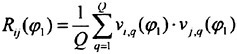
(4)
where Q is the total number of couples of velocities acquired simultaneously. Reynolds stresses evaluation
is worked out basing upon results get by the ATT, collecting 200 samples for each selected angular position.
3. WAKE ANALYSIS
3.1 Trailing Edge Wake
Angular variations of the phase averaged mean axial velocity in the first measurement disk are shown in figure 6. The velocity is periodical, with the repetition at the blade passage frequency of four characteristic profiles, which are originated by the blade flow. The differences among these four velocity profiles are explained as an effect of differences in the local hydrodynamic operation among the blades, due to geometrical imperfections, rather than as the result of measurements uncertainties.
3.1.1 Blade Viscous Wake and Trailing Vorticity
The viscous wake due to the boundary layer on the blade is represented by the defects in the velocity. Figure 6 shows the axial component of the velocity defect in the trailing edge wake. The axial and the tangential components of the defect are the largest, but as an effect of the contraction of the slipstream, a small amount of the velocity is present in the radial velocity too. It can be noticed in figure 7, where some circumferential variations of the radial velocity Vr are presented.
The Vx peak at r/R=0.9 is due to the presence of the tip vortex, which formed at the blade tip and moved inboard for the slipstream contraction. Tip rollup core is in fact characterized by pressure decay and flow acceleration along the vortex line, as will be discussed in more detail in the analysis of the near wake. Outside the propeller slipstream (r/R=0.95 and r/R=1.05), the Vx circumferential variations show an opposite phase oscillation with respect to those inside the slipstream. Furthermore, the velocity profile at r/R=1.05 can be considered representative of an inviscid flow.
The trailing vorticity, shed from the blade trailing edge, is pointed out by the jump in the Vr, shown in figure 7. This jump, which is modeled with no thickness according to a potential theory, is instead actually widespread over a finite thickness as an effect of the viscous and turbulent diffusion in a real flow. The amplitude of the velocity change, which is representative of the radial gradient of the bound circulation, increases moving from the mid-span sections of the blade toward the tip and the root, where maximum values are reached. The switch in the vorticity sign, corresponding to the maximum of the circulation along the blade span, is located at about r/R=0.6. At this radius the angular profile of the radial velocity is rather flat, with only a velocity defect due to the viscous wake.
The Vx distributions on the trailing edge measurement disk is sketched in the left half of figure 8. In the root region deeper axial velocity defects are measured. A neighboring region of slow flow, which extends in the pressure side of the blade, can be also noticed. This flow distribution in the inner radii is due to the increasing thickness of the blade sections toward the root, as well as to the fact that the LDV measurement points are closer to the blade trailing edge.
The mean velocity gradients show that tip vortex is located in the suction side of the blade wake at the trailing edge. Flow visualizations (figure 12), confirms that tip vortex convects over the blade suction side as soon as it formed at the tip. For blades with zero chord length at tip, this flow behavior is in agreement with the general understanding about effects of the blade geometry on the tip vortex formation and evolution (1).
In the adopted test conditions, the highest axial flow accelerations and the thinnest viscous wake deficits along the blade wake from the hub to the tip occur in the radial stations around r/R=0.7. It means that the corresponding blade sections are the most efficient for propeller thrust generation.
3.1.2 Turbulent wake
The axial component of the phase averaged turbulent wake at the trailing edge is shown in the right half of figure 8, where the distribution of the axial velocity standard deviation σx is sketched. The axial turbulence enables to point out very well the shape of the blade wake and the tip vortex core movement toward the suction side, which causes an abrupt curling of the σx distribution at the tip.
The maximum value of the turbulent intensity σx/V∞ at the trailing edge is about 20% in the tip vortex core. The spiraling process, which occurs very close to the blade, is highly turbulent since it produces strong mean velocity gradients and involves the blade boundary layer flow.
Along the blade wake, the highest axial fluctuations are measured at the root sections, where σx/V∞=10÷14%. The radial variation of the axial turbulent intensity has instead a minimum around r/R=0.7. These features of the axial turbulent wake distribution are strictly correlated with those previously focused by looking at the mean velocity distribution in the corresponding regions of the blade wake.
The axial turbulence distribution enables to point out the effects of the propeller hub in a certain detail. In fact, its boundary layer causes an irregularly bounded region of high σx around the hub, composed of radial peaks spreading outwards. Outside the hub and
the blade wake, axial turbulent intensity reduces at the free stream levels (σx/V∞=2%).
In order to perform a deep analysis of the turbulent wake features, the velocity probability density functions (PDF) and the skewness were calculated in the trailing edge wake. The skewness angular variations (figure 9.a) in the blade wake is generally negative, with two peaks located besides the turbulent wake center, which in this research is defined as the angular position where σx is maximum. Considering a velocity PDF evaluated in the suction side of the blade wake (figure 9.b), an asymmetrical profile can be noticed due to the presence of samples corresponding to a slower axial flow, which cause a gradually decreasing tail. This shape reveals the presence of blade wake unsteadiness and local flow separations, particularly important in the suction side of the blade, where the minimum skewness is measured. The low value of the skewness modulus in the wake center means a less unsteady flow with more symmetrical PDF. To verify that the adopted ε is suitable to resolve the spatial velocity gradients, an angular resolution of ε=1° has been also tested, giving result similar to those obtained for ε=2°.
Far from the blade wake, both inside (r/R=0.7, figure 9.c) and outside (r/R=1, figure 9.d) propeller slipstream, the velocity PDF are symmetrical, but not strictly Gaussian. These PDF shapes are identical to those measured for the free stream in the test section. This result indicates that the turbulence observed in these wake regions is due to the upstream flow and not produced by the propeller blades.
The implemented ATT was applied to work out evaluations of the Reynolds stresses, since it provides both suitable accuracy for such calculations as well as samples referred to the selected angular position φ1, according to the (4). In figure 10 the Reynolds stresses for the fluctuating components of the velocity vx and vr, evaluated at an angular position in the blade wake and at another one far from blade flow are compared. The x-component Rxx and the r-component Rrr of the Reynolds stresses tensor are dominant with respect to the cross one Rxr. The blade wake turbulence produces Reynolds stresses 2 orders of magnitude larger than the ones of the undisturbed flow, where the cross component Rxr is practically null.
3.1.2 Spatial Separation of the viscous, potential and turbulent wakes.
In figure 11 the traces of the locations where (i) the minimum mean axial velocity defect, (ii) the center of the radial velocity jump and (iii) the peak of the turbulent intensity occur are plotted. They are indicative respectively of the mean surfaces of (i) the viscous wake, (ii) the trailing vortex sheet (potential wake) and (iii) the turbulent wake. As wake thickness is not null in a real flow, mean surfaces are used for representing the wake. The traces of both the turbulent wake and the viscous wake are close positioned. The potential wake has instead a larger curvature toward the suction side, particularly at the tip region. This feature, which was also observed by Kobayashy (2), is interpreted as an effect of the roll-up process. These considerations indicate that, with the adopted definitions, a spatial separation between the viscous and the potential wake can be resolved.
3.2 Near Wake Evolution
To introduce wake evolution analysis a visualization of the near wake vortices structure, realized in incipient cavitating flow conditions, is shown in figure 12. The tip vortex evolves along helicoidal paths, as it separates from the blade tip. The strong and thick axial vortex, starting from the hub tip, is generated by the vorticity produced at the root of the blades, which flows on the hub surface and grows into a vortex structure.
3.2.1 Wake Geometry
In marine propeller theories, an accurate evaluation of the wake-induced velocity field on the blade is a key factor for performance prediction. This is primarily due to the low aspect ratio and the skew of marine propellers, which cause strong three-dimensional effects. The knowledge of the wake geometry along downstream convection from the blade trailing edge is required in order to fulfill this goal.
The Vx and σx distributions on the five measurement disks are shown in figure 13 and 14. From a geometrical point of view, downstream wake evolution is characterized by a progressive bending of the blade wake surfaces. This is the effect of radial variations of the wake pitch, induced by the cross flow. In the mean axial velocity distribution, the trajectory of the tip vortex causes an angular displacement between tip vortex and the inboard blade wake, which increases moving downstream. The turbulent wake instead preserves better the original link between the tip vortex and the inboard blade wake within the near wake. In fact, the σx distribution shows a continuos curved blade wake trace, which ends into the tip vortex.
A quantitative description of the blade wake geometry in the near wake is proposed in figure 15, where the angular positions of the σx peaks in the five measurement planes for some radial stations are plotted. The slope of the locus represents the pitch angle. The almost linear variation of the traces means that a nearly constant pitch occurs during wake downstream convection. By comparing the above traces with the propeller constant pitch angle, it is shown that wake pitch equals the geometrical one in the mid-span
sections of the blade (around r/R=0.7). Significant pitch differences are measured between the blade tip sections and the root ones. This is the cause of the large wake angular dispersion.
A second factor of the wake geometrical characterization is the contraction of the slipstream, which is the effect of the axial flow acceleration. In figure 16 the radial variations of the mean axial velocity for different angles in the trailing edge flow are shown. The figure indicates that the slipstream axial acceleration stops, that is Vx/Vinf=1, at the same radius along the circumference. In view of this angular uniformity of the slipstream radius, its transversal shape is a circumference. This feature suggests considering the propeller slipstream basing on the simplified concept of a stream tube, in analogy with that defined according to a momentum theory of propellers. Nevertheless, from the third measurement disk (r/R=1.15), the radius of the stream tube varies along the circumference, meaning that its transversal contour is distorting with respect to the initial circumference. In the present tests, the maximum range of this radius variation along the circumference is about 0.08 r/R and occurs in the disk at X/R=1.15.
In view of this angular variation, the previous defined radius is not suitable for the aim of representing the slipstream contraction. Alternatively, the radius where the axial flow inside the tip vortex reaches the condition of Vx/Vinf=1 is adopted. This slipstream radius will be indicated as rS. This choice enables to compare the deduced ultimate contraction with the results obtained by Min (7). Min used the radial location of the tip vortex for evaluating the radius of the slipstream of many propellers, which were driven from upstream as in the experimental arrangement available for the present research. The deduced slipstream shape is shown in figure 17. It is characterized by a very high rate of contraction in the neighborhood of the propeller and is practically complete within the first diameter. The asymptotic radius of the contraction is rS/R=0.82÷0.83. This value is in agreement with that adopted in some empirical wake models (r/R=0.83), basing on Min’s measurements.
3.2.2 Turbulent Diffusion and Viscous Dissipation
Strong processes of turbulent diffusion of momentum and viscous dissipation of energy occur within the investigated region. These processes produce broadening and decay of the mean velocity defects, as shown in figure 18.a, which presents the detail of the downstream modification of the Vx defect at r/R=0.7. These effects are particularly marked in the hub and blade turbulent wakes, which are rapidly faded. Figure 18.b shows the modification of the σx at r/R=0.7, in the five measurement disks. In the tip vortex flow, a different trend is instead observed (figure 14): the greater is the distance from propeller, the higher is its turbulence intensity. These opposite characteristics of the axial turbulence evolution, concerning the effects of the diffusion and the dissipation processes, can be explained considering the different nature of the hub and blade turbulence in comparison with that of the tip vortex. Being generated by a boundary layer flow, the hub and blade turbulent flow is composed of small-scale eddies, where the dissipation processes are effective. On the other hand, the highest turbulent energy content in the tip vortex is on the large-scale eddies. The downstream increase of the σx as well as the enlargement of the tip vortex core can be considered as an effect of the strong mean velocity gradients and the spiraling of the blade boundary layer in the roll-up process. However, a significant contribution to the resulting σx is also given by the unsteady spatial oscillations of the slipstream.
The processes of diffusion also influence the evolution of the trailing vorticity. The comparison of some circumferential variations of the Vr at X/R=0.65 and X/R=2.15, presented in figure 19, shows that the Vr jumps are gradually spread over increasing angular intervals while their amplitude reduces. At X/R=2.15, the large velocity jump of the Vr, observed in the profiles at r/R=0.8–0.85, is due to the tip vortex passage.
3.2.3 Roll-up Process
A first feature of the roll-up process can be highlighted comparing the induced Vr jumps at r/R=0.9 in the trailing edge (X/R=0.2) and at x/R=0.65. At X/R=0.2 (figure 7) the jump is composed of two linear variations, divided by a flat central part, while at X/R=0.65 it presents an almost linear trend (figure 19). This change indicates that the roll-up is progressively growing into a classic Rankine vortex structure, as it develops from the tip of the blade.
In the cross flow velocity field, represented in the fixed frame at X/R=1.15 and sketched in figure 20, the general trend of the slipstream to swirl and to contract can be qualitatively resolved. The high induced velocities at the tip region in the cross flow represent the effect of the roll-up process, in the root sections, the presence of the hub does not allow the development of individual root vortex structures
Useful information to analyze roll-up process can be also deduced representing the velocity field in a rotating frame Ο’-s,r,φ, where r and φ are the ones shown in figure 4, while s is along the blade pitch direction (indicated by the pitch angle ![]() ). The pitchline velocity VS can be computed by:
). The pitchline velocity VS can be computed by:
(5)
This representation is suitable to relate the propeller blade flow to that of a planar wing in stationary conditions. In figure 21, the pitchline velocity field at X/R=1.15 is shown. In the tip vortex core a pitchline velocity maximum can be noticed, corresponding to that observed in wing tip vortex (11),(12). Around the tip vortex core a pitchline velocity defect is located. It seems to indicate that the viscous wake is involved in the spiraling process, confirming previous studies based on LDV results, which highlighted the effects of the viscosity in the roll-up process (1),(2).
3.3 Slipstream Instability and Far Wake Breakdown
The visualization in figure 12 shows that the hub and the tip vortex flows are in completely developed cavitation conditions. Only small regions of laminar cavitation, which occurs at the leading edge of the blade, instead characterize the blade flow. This hydrodynamic feature of the tested propeller is primarily due to the spanwise distribution of the circulation on the blade, which produces a strong vorticity at the root and the tip. The consequent roll-up process implies marked pressure decay inside its core, where the conditions for cavitating flow are firstly reached. Such hydrodynamic behavior of the tested propeller is useful to analyze the processes of the slipstream instability and the vortices breakdown, because the tip and the hub vortices can be easily visualized and followed. Dissertations on the similar unstable nature of the far wake for aeronautical rotors are provided in (13).
In figure 12, a local distortion in the path of the tip vortex is pointed out. By means of numerous similar visualizations, it was experienced that these imperfections occur in a random manner. Furthermore, the greater is the distance from propeller, the higher is their number and amplitude.
A second aspect of the unsteady spatial deformation of the wake, with respect to the ideal helicoidal geometry, was focused through the direct inspection of the wake in the test section, using stroboscopic light, as well as trough the visualizations obtained using camera exposure some propeller revolution periods long. It consists in the fluctuations in the radial direction of the hub and tip vortices system, behaving as a single, rigid structure. The amplitude of these fluctuations increases along the downstream evolution.
These two features of wake evolution, which have been pointed out considering a local and a global perspective, characterize the onset of the unstable process which leads to the wake breakdown.
The manner in which the breakdown of the hub and the tip vortices develops in the far wake proved to depend on the propeller loading conditions. From a general point of view, for low advanced ratios J (propeller highly loaded) flow visualizations show that a strong spatial distortion sharp occurs in the helicoidal vortices system during its evolution (figure 22). In particular, it was observed that two helicoidal tip vortices tend suddenly to overcome and interlace each other. Behind this region of high distortion of the helicoidal system, the breakdown of the tip vortices occurs. Moreover, at the axial station where the strong distortion of the tip vortices system takes place, the straight trajectory of the axial vortex grows into a spiral, whose pitch decreases downstream until its breakdown (figure 23).
On the other hand, for high advanced ratios (propeller lowly loaded) the downstream increase of both local distortions and slipstream spatial fluctuations is more gradual (figure 24). It was experienced that the higher is the propeller advanced ratio J, the more the breakdown process is moved downstream.
The analysis of the LDV measurements results can provide quantitative information on the processes of the near wake unsteady deformations and vibrations. A concise dissertation on this concern is proposed below.
The angular variation of the radial turbulence in the tip regions shows high values of the σr for a large angular interval, in addition to the peak due to the tip vortex passage (see figure 25.a)1. This feature, which is observed only in the radial turbulence, reveals the unsteady fluctuations of the whole slipstream in the radial direction, which have been previously observed through the visualizations. Moreover, in the trailing edge measurement disk, the angular variation of the σr at the boundary of the slipstream with the outer flow (r/R=0.9) is rather smooth and the minimum values of the turbulence intensity reduces at almost the free stream level 2%. One diameter behind propeller, as shown in figure 25.b, these two features change: many oscillations occur in the angular variation corresponding to the boundary region (r/R=0.8–0.85) and the minimum values of the turbulent intensity increases up to about σr/V∞=5÷6%. The angular variations of the other two turbulence components, here not shown for brevity, present a similar trend (increasing oscillations and higher minimum values of the σ) at the boundary of the slipstream. This result proves that with downstream evolution not only the slipstream fluctuations grow, but also that a rising complexity of its boundary region with the external flow develops. In particular, the quasi periodic oscillations of the turbulence angular variations suggest the onset of transition process to vortex breakdown. To such concerns appear also to be referred the downstream distortion of the traversal shape of the
stream tube and the complexity of the mean velocity distribution at the transition region, which were previously discussed in the near wake analysis.
Another difference at the X/R=2.15 axial plane, with respect to the trailing edge features, is exhibited by the σr angular variations in the inner radii (r/R=0.25–0.3). The corresponding σr are very high and their profiles are irregular and oscillating, as an effect of the distortion and the unsteady fluctuations of the axial vortex.
Further investigations of these aspects are required in order to explain the relation between the velocity field at the slipstream boundary and the far wake process of high distortion and breakdown as well as to assess the dependence of these processes on propeller loading conditions and geometry.
4. CONCLUSIONS
The results of the investigation of a marine propeller wake by means of LDV and complementary by flow visualizations were presented and discussed. The analysis was focus on the downstream evolution features.
In the trailing edge flow, the viscous wake, the trailing vorticity and the turbulent wake were resolved. Their survey, just behind propeller, enabled to point out the blade local hydrodynamic operation as well as the hub effects.
The LDV results in the near wake showed that the actual blade wake geometry is significantly deformed with respect to the classical undistorted wake models (6), based on rigid helical surfaces shed from the blades. This aspect was examined through the evaluation of both the blade wake and tip vortex pitch, along with the contraction of the slipstream. Strong processes of viscous dissipation and turbulent diffusion were also observed. The relative displacement between the tip vortex and inboard blade wake along with the processes of dissipation and diffusion should reduce the contribution of the blade vorticity to the roll-up process, in comparison with that predicted using undistorted wake models and potential flow representation. The tip roll-up flow and the viscous effects in the spiraling process were also highlighted. Aiming to deeper descriptions of this complex and extremely turbulent flow region, whose precise modeling holds great interest for numerical applications, higher spatial resolution and accurate LDV results will be required.
In the far wake, visualizations of the cavitating hub and tip vortices system were used to show the slipstream unsteady fluctuations and the final vortices breakdown. Also, the LDV measurements give averaged information on the process of destabilization of the vortices systems throughout quasi periodical azimuthal oscillations. Further quantitative analyses of such phenomenon by LDV and especially PIV, which enables to account for flow unsteadiness, are considered to be future works.
ACKNOWLEDGEMENTS
The authors are grateful to Mr. De Clementi for the realisation of the instrument to analyse encoder signals, to Dr. Esposito for his contribution in wake measurements graphical visualisation and to Mr. Guerra for the propeller flow visualisations. The authors also would like to express their gratitude to the C.E.I.M.M. staff for his precious co-operation.
REFERENCES
1. Jessup S.D. “An experimental investigation of viscous aspects of propeller blade flow”, Ph.D. Thesis—The Catholic University of America, Washington D.C., 1989.
2. Kobayashi S. “Propeller wake survey by laser-Doppler velocimeter”, Proc. of the International Symposium on the Application of laser-Doppler Anemometry to Fluid mechanics, Lisbon, 1982.
3. Kobayashi S. “Experimental methods for the prediction of the effects of viscosity on propeller performance”, Dep. of Ocean Engineering, Rep. 81–7 MIT, 1981.
4. Wang M.H. “Hub effects in propeller design and analysis”, MIT Ocean Engineering Dep., Rep. 85–14, 1985.
5. Hoshino T. “Hydrodynamic analysis of propellers in steady flow using a surface panel method”, Journal of the Society of Naval Architects of Japan, 1989.
6. Landgrebe A.J., Cheney M.C. “Rotor wakes—Key to performance predictions”, AGARD, CP 111, 1972.
7. Min. K.S. “Numerical and Experimental methods for prediction of field point velocities around propeller blades”, MIT Ocean Engineering Dep., Rep. 78–12, 1978.
8. Hoshino T., Oshima A. “Measurement of flow field around propeller by using a 3-component laser Doppler velocimeter”. Mitsubishi Technical Review, Vol. 24, No. 1, 1987.
9. Cenedese A., Accardo L., Milone R. “Phase sampling techniques in the analysis of a propeller wake”, International Conference on Laser Anemometry Advances and Application, Manchester (UK), 1985.
10. Stella A, Guj G., Di Felice F. Elefante M. & Matera F. “Propeller wake analysis by means of LDV phase sampling techniques”, Proc. of the 3th International Symposium on Cavitation, Grenoble, 1998.
11. Cenedese A., Accardo L., Cioffi F. “Experimental analysis of tip vortex by laser-Doppler anemometry”, Proc. of the II International Conference on Application of laser-Doppler Anemometry to Fluid mechanics, Lisbon, 1984
12. Batcehlor G.K. “Axial flow in trailing line vortices”, Journal of Fluid Mechanics 20, 1960.
13. Landgebe A.J. “An analytical and experimental investigation of helicopter rotor hover performance and wake geometry characteristics”., USAAMRDL technical report 71–24, Eustis Directorate, U.S. Army Air mobility Research and development Laboratory, Fort Eustis, 1971.
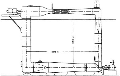
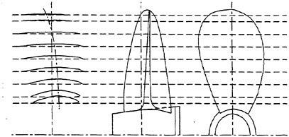
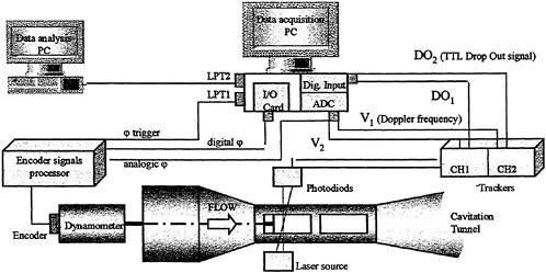
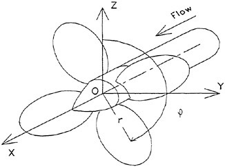
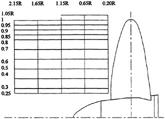
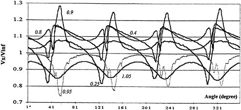
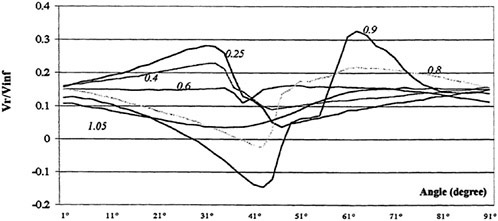
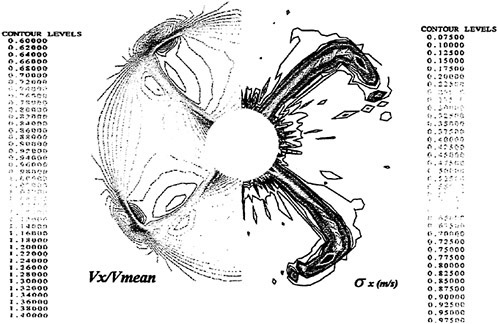
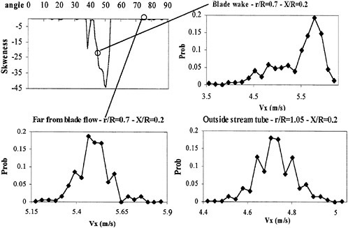
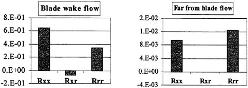
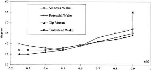
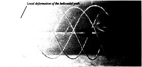
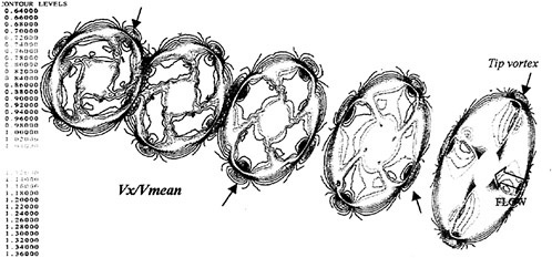
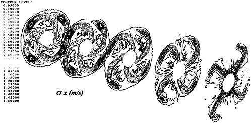
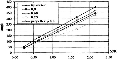
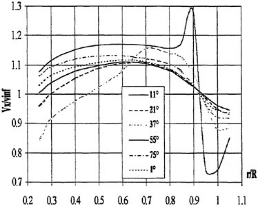
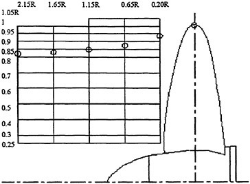
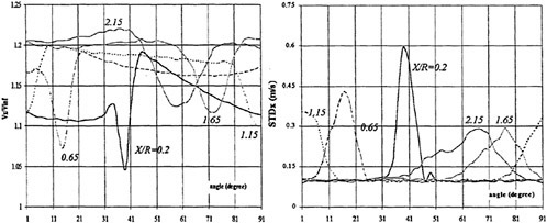
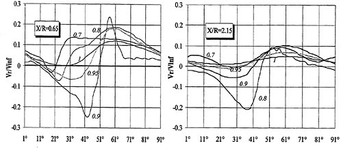
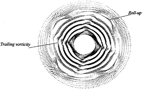
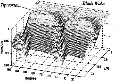
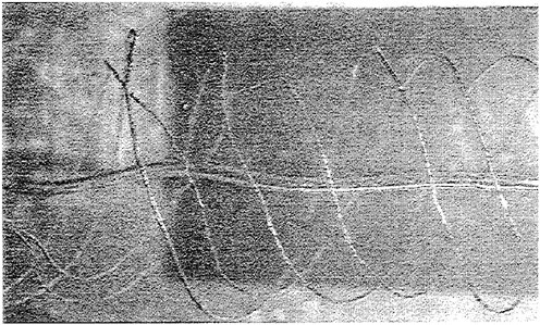
Figure 22. Strong deformations of the helicoidal paths of the tip vortices. J=0.62. 3÷5 diameters behind propeller.
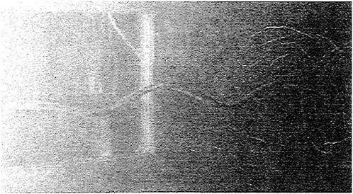
Figure 23. Breakdown of the tip vortices system. Strong deformation of the axial vortex. J=0.62. 6÷7 diameters behind propeller.
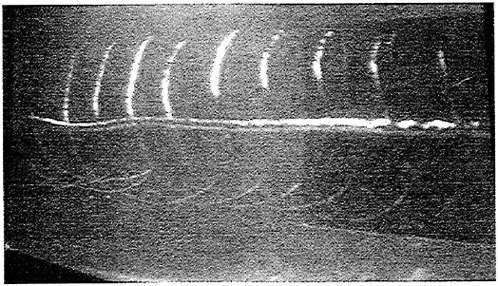
Figure 24. Deformation of hub and tip vortices system. J=0.88. 4÷6.5 diameters behind propeller.
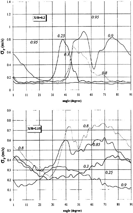
Figure 25. a b. Angular variations of the σr at Χ/R=0.2 and X/R=2.15
DISCUSSION
A.Cenedese
Rome University “La Sapienza,” Italy
In 1985 I was working at C.E.I.M.M. implementing an experimental set-up for the measurement of the velocity field in the wake of operating marine propellers (see reference 9 of the paper). I am pleased to see that 12 years later a sort of continuation of that work has been realized.
Among other things, a first interesting aspect which rises looking at the past and the present work is the impact of upgrading the experimental facilities on results of these kinds of investigations, enabled by the technical evolution of recent years. I used the same two-component LDV system with trackers which has been used by the authors. However, this is the only common part between the measurement chain implemented for that work and the present one. In 1985, a recorder Ampex, an A/D converter and a PDP 11/24 digital computer were used for data acquisition and analysis. This limited the data quantity to be stored and used for the statistical analysis of propeller turbulent flowfield. LDV data validation through the control of tracker TTL drop out signal (indicated
as validation signal VS in the paper) was not possible. Phase sampling was based on the correspondence between time instants and propeller angular positions, using a trigger signal provided once per revolution. These limitations are overcame in this work, so increasing both the amount of data for describing the velocity field as well as their accuracy.
A second interesting aspect of the work is the idea of using the TTL validation signal, provided by the trackers, to trigger the acquisition of LDV samples. The data acquisition technique, developed following this triggering procedure, proved to give a high measurement efficiency in poor flow seeding conditions. The consequent time saving appears to be very important from a practical point of view, giving the opportunity to perform a second measurement campaign to measure the third component of the velocity. I believe that these kinds of results are very helpful for understanding the complex propeller hydrodynamics.
Finally, I would like to ask the authors to explain with greater detail what kinds of problems have arisen using a frequency tracker for analyzing a Doppler signal which is composed of individual bursts, that is, an opposite situation with respect to that suitable for the tracker ideal operation.
AUTHORS’ REPLY
Primarily, we would like to thank Prof. Cenedese for his interesting observations about our work. His activity at C.E.I.M.M. in 1985 has actually represented the prime reference point for the development of the present research.
Replying to Prof. Cenedese’s question, we can argue that the condition of poor fluid seeding was determined by the fact that contemporary tests of propeller cavitation performance were executed at C.E.I.M.M., during the carrying out of our work. The high levels of signal to noise ratios, provided by the LDV system optical configuration, particularly for the forward scatter way of operation, allowed the tracker to start tracking the Doppler frequency after very few cycles of a burst. In other words, the tracker way of operating is similar to that of a counter. This measurement condition suggested implementation of a data acquisition technique, the so-called tracking triggering technique, where the condition of tracker following the Doppler frequency is used to trigger the LDV data collection. This avoids acquisition of invalid samples, reducing the total measurement time.
DISCUSSION
S.Jessup
Naval Surface Warfare Center, Carderock Division, USA
The authors should be congratulated for performing the detailed analysis of the downstream wake structure of the operating propeller. The availability of a long test section allows study of the far wake. The use of LDV in the study of the far wake, as the authors have discovered, is difficult due to the passage of the blade’s wake downstream in the turbulent flow field of the water tunnel. It would be nice to perform such an investigation in a tow tank, in absolutely still water, where the freestream turbulence was nonexistent. As the wake progresses downstream, the influence of the freestream turbulence is to move the wake about on a trajectory which is randomly perturbed with time, so that as distance downstream increases, each flash of the strobe light shows the cavitating vortex in a difficult location. One should remember that vorticity is a material quantity, which will “go with the flow.” This can be observed, hopefully, on the tour Wednesday in the DTMB 36” water tunnel. In measurements in our tunnel, LDV of detailed wake structure beyond X/R=1.0 is not pursued due to wake structure wandering. The degree of vortex wandering was qualitatively determined by observing the cavitating vortex with a crosshair telescope illuminated with strobelights. Movement of the vortex must be well within the core diameter.
An assuredly incomplete list of causes of vortex wandering could be postulated:
-
Mean flow spatial variations and turbulence generated by in-tunnel wake producers.
-
Freestream turbulence
-
Turbulence generated by the blade surface, which passes into the wake and tip vortex.
-
Variations in self induction, primarily due to the variations in the tip vortex strength and location.
Item one is the most obvious effect, which is not applicable, but which causes the largest perturbation of the downstream wake. This is easily observed when propellers operate behind model hulls, upstream struts, vanes or screen wake producers. I would hypo-thesize that items 2 through 4 are prioritized in order of importance. Unfortunately it is difficult to separate out the various effects with LDV measurements.
I agree with the authors that the use of PIV is the obvious choice to capture individual vortex structures far downstream. We are slowly attempting to develop such a system for water tunnel use. For propulsors operating in highly turbulent flow this may be the only way to fully capture the structural details of the vortex. A question I can pose to the authors is whether the tunnel itself causes any of the oscillatory behavior of the tip and hub vortex. If so, is this dependent on the test section type, i.e., closed or open test section?
Finally, I would like to thank the authors for the pursuit of these types of measurements. We have made a significant commitment over the years in support of LDV. The challenge is to use the tool effectively to stimulate research and the resolution of engineering problems. The burden often lands on the analyst to convert the raw data to useful conclusions, which the authors have effectively performed.
AUTHORS’ REPLY
We would like to thank Dr. Jessup very much for the detailed review of the paper, the important comments on our work and suggestions for future research concerning the development of propeller wake vortices system breakdown.
We agree with the analysis of the influence of the background turbulence, which produces the oscillations and deformation of the helicoydal tip and axial hub vortices, during downstream convection of the wake. Even if the mean flow spatial variations and turbulence generated by in-tunnel wake producers and freestream turbulence are very important perturbations, we believe that the oscillations and the successive destabilization leading to vortex breakdown are generated by the variation in self-induction. As a matter of fact, we can suppose that the behavior of a helicoidal vortex does not differ too much from that of a series of vortex rings. It is well known that for this simpler situation, both numerical simula-tions (1) and accurate experiments in tow tanks prove the destabilization occurs by two different mechanisms: azimuthal instability and leap-frogging pairing, depending on the value of the governing parameters. The present experimental results suggest the conjecture that the dominant form of destabilization is the azimuthal one.
Replying to the final question, for our experience the process of slipstream instability and final breakdown is considered to be independent of the tunnel features for low test section blockage ratios. Nevertheless, in the open jet configurations the behavior of propeller wake vortices can be strongly affected by the turbulent mixing layer for high blockage ratios, if the helicoidal vortices structure develops outside the potential jet core in the final stage of its evolution.
Reference
[1] Shariff, K., Verzicco, R., Orlandi, P., “A numerical study of three-dimensional vortex ring instabilities: viscous corrections and early nonlinear stage,” J. Fluid Mech., 1994, vol. 279, pp. 351–375.
Numerical Simulation of Tip Vortices Roll-Up
X.Viot, D.Fruman (École Nationale Supérieure de Techniques Avancées, France)
F.Deniset, J.Billard (École Navale, France)
ABSTRACT
The objective of this paper is to test the ability of two commercially available Reynolds Averaged Navier-Stokes (RANS) codes, based on finite volume algorithms—STAR CD™ and FLUENT-UNS™, the unstructured version of FLUENT™—with improved spatial resolution along the path of the tip vortex and at the tip of the wing, various turbulence models, convection schemes, and exit boundary conditions, to predict the tip vortex flow in the very near region of an elliptical wing. The computations were conducted for a large angle of attack of the foil, because it allows to test the ability of the code to model high lift coefficient situations, such as those occurring on jumbo airplane wings during the phases of take-off and landing. Moreover, if this extreme condition is properly modelled it can be expected that the code will provide acceptable results for moderate angles of attack encountered in hydrodynamic applications.
The results issued from the numerical codes are compared with experimental results, tangential and axial velocity profiles obtained at positions as close as 0.1 mid-span chord from the tip. In particular, the vortex intensity and core radius along the vortex path are systematically compared.
The comparison between numerical predictions and experimental results shows that the diffusion of the tip vortex is over predicted by the two codes whatever the turbulence models and mesh refinements. However, it is clearly shown that a higher order convection scheme and a non linear turbulence model improve significantly the results.
Whatever the discrepancies between the experimental and the numerical results, the analysis of the latter show that the methodology used by the Action Concertée Cavitation partners to estimate the pressure on the vortex axis, based on the assumption that the vortex is axisymmetric even in the very near region, is fully justified.
NOMENCLATURE
|
a |
tip vortex core radius |
|
C |
mid span chord |
|
Cℓ |
lift coefficient |
|
Cp |
pressure coefficient |
|
Cp0 |
pressure coefficient at the tip vortex center |
|
Cp0Lamb |
Cp0 predicted by the Lamb profile |
|
Cp0num |
Cp0 predicted directly by the code |
|
k |
turbulence intensity |
|
P∞ |
free stream pressure |
|
P0 |
tip vortex center pressure |
|
Plc |
local cut-off pressure |
|
r |
local radius |
|
V∞ |
free stream velocity |
|
Va |
axial velocity |
|
Vt |
tangential velocity |
|
x |
axial coordinate |
|
y |
spanwise coordinate |
|
y+ |
non-dimensional distance to the wall |
|
z |
vertical coordinate |
|
ε |
turbulence dissipation rate |
|
ν |
kinematic viscosity |
|
ρ |
liquid density |
|
σ |
cavitation number |
1 INTRODUCTION
Numerical computation using Reynolds Averaged Navier Stokes (RANS, [1]) codes of the flow field of complete airplanes requires a very good representation of the roll-up and development of the vortices issued from the tip of the wings or at the discontinuity between flaps and wing during the take-off and landing operations. Indeed, these vortices are particularly strong because, to generate the required lift at low speeds, they develop, by Blasius theorem, a very large circulation. Moreover, since they may occur at short distances from the body, they will strongly interact with it and with the downstream lifting surfaces. These interactions are confined to relatively short, in terms of foil chords, distances downstream, in regions where the roll-up of the vortices is not necessarily completed. A good knowledge of the evolution of the vortex intensity and of the core dimension (region where the viscous effects are predominant) along its path is therefore essential and has to be simulated correctly by any RANS code. Moreover, in naval practice, it has been by now very well documented that tip vortex cavitation (TVC) of hydrofoils and propeller blades occur at very short distances, of the order of magnitude of one tenth of a chord, from the tip. In this region the tip vortex is far from being developed and both, the vortex intensity and core diameters vary rather quickly. Again, accurate prediction of TVC requires RANS codes which properly account for the peculiarities of vortex flows and, more precisely, of turbulence in rotating flows.
The reasons of the difficulties associated with a correct modelisation of the tip vortex are,
-
the dimensions of the core, where the tangential velocities vary very rapidly, with velocity gradients as high as 104 s−1, is two orders of magnitude or less smaller than the foil chord, therefore, the mesh has to be refined substantially in this region to achieve a good enough spatial resolution,
-
the position of the vortex path is a priori unknown and has to be determined by successive approximations,
-
the tip vortices remain coherent over very long distances and the free stream conditions are not recovered downstream within reasonable domain dimensions, thus, the boundary condition on the downstream limiting surface is unknown a priori.
Other reasons are directly related to the modelling of turbulence at very high Reynolds numbers in intense rotating flows. The usual turbulence models are well adapted to boundary layer situations but ill fitted to the presently discussed flow conditions of what can be called free turbulence. Indeed, in the case of the tip vortex, the fluid occupying the boundary layer on the tip region of the foil surface is swept away in rotation by the outer potential flow and carried on, with its vorticity, into the vortex core. This vorticity can only decay in the absence of sources of production other than a solid boundary or a forced shear layer (such as in a jet). This phenomenological reasoning may explain the very slow diffusion of tip vortices even at very large Reynolds numbers.
Many authors noticed the influence on the tip vortex over-diffusion of the downstream extension of the mesh and of the outlet boundary condition.
Dupont et al. [2] computed the flow field of an elliptic planform hydrofoil having a NACA 16020 cross section using the commercially available FIDAP™ and TASC-FLOW™ codes with implemented k-ε turbulence models. The authors obtained maximum tangential velocities larger than the experimental ones at the tip of the foil. However, they dropped drastically downstream and, at a distance of only 0.125 of the maximum chord, they were reduced to about 60% of the experimental values. By improving the spatial resolution, the TASC-FLOW™ code raised the tangential velocities, both at the tip and at 0.125 chord without reaching the experimental values. At 0.5 chord, the prediction is, whatever the code, less than 50% of the experiment. Even if the tangential velocities are over predicted at the tip, they drop drastically downstream indicating a significant growth of the core dimension as compared to the experimental values. Moreover, the authors demonstrated that even in a diffusing axisymmetric vortex the theoretical solution of Lamb for laminar flows [2] was not obtained and the diffusion was over-predicted.
Deniset [3] conducted computations using the FLUENT™ code for the same elliptical planform hydrofoil with aspect ratio of 3.82 and a NACA 16020 symmetric cross section, at an incidence angle of 8°, a Reynolds number 8.4×10⁵ and, as Eça et al. [4], a constant pressure boundary condition at the outlet. The asymmetric character of the tip vortex in the region close to the tip has been highlighted. The author has shown that the excessive increase of the core radius prevents from a correct prediction of the static pressure in the viscous core.
Use of specifically developed computer codes did not improve the results as shown by the work of Dacles-Mariani et al. [5]. A rectangular half-wing with a NACA 0012 airfoil section was tested. They used INS3D-UP, a three-dimensional, incompressible Navier-Stokes flow solver, with a modified one-equation turbulence model, an accurate convection scheme of fifth-order, a grid of 1.5 million points. They set first a Dirichlet condition in the downstream section of the computational volume (at 0.69 chord of the trailing edge) and observed a jump in the different quantities evaluated in this region. When setting a Neumann outflow pressure boundary condition at the exit, as determined by three components laser measurements, they get a good agreement between the profiles of the measured and the computed modulus of
the velocity vector through the vortex. However, this does not insure a correct prediction of the tangential velocity profiles and justifies the under-prediction of the core static pressure. The latter is ascribed to the inadequation of the turbulence model. Although the numerical dissipation was essentially reduced by the improved spatial resolution and the modified turbulence model, the diffusion of the vortex was still overpredicted. Moreover, use of an experimentally defined boundary condition coupled to the numerical code can not be considered as a satisfactory practice for prediction purposes.
To summarize, all the attempts made with commercial and non commercial RANS codes to determine the flow field issued from an elliptical or rectangular foil have over-predicted the diffusion of the vortex core, even in the very near region within one mid-span chord from the tip.
2 FOIL GEOMETRY AND PROCEDURES
The hydrofoil used in the computations and the experiments had an elliptical planform of area ratio 3.82 and a NACA 0020 symetric cross section. The computational domain was limited laterally by surfaces simulating the walls of the cavitation tunnel test section, 8 cm wide and 15 cm height, where the experiments were conducted. The computations were carried out for an incidence angle of 10° and a Reynolds number of 4×10⁵.
The axial and tangential components of the velocity field in the tip vortex region were measured by means of a DANTEC two components laser Doppler anemometer operating on the backscattering mode [6].
In order to allow for comparison between the experimental and the computational results, a procedure of analysis of the data identical to the one used in previous works ([7], [8]) was adopted. It consisted in the extraction, from the computed flow field, of tangential and axial velocity profiles along a line parallel to the span of the hydrofoil centred on the local axis of the tip vortex, Figure 1. The position of the tip vortex axis was localized by searching, first, the minimum of the pressure in each plane normal to the free stream velocity, and, then, by searching the zero of the tangential velocity along a vertical line very close to the minimum pressure location. Both methods lead to the same position.
The tangential velocity profiles were fitted using a Lamb velocity profile,
where Vt is the tangential component of the velocity, Γ is the circulation or vortex intensity, a is the radial distance (core radius) at which the maximum tangential velocity is achieved and r is the radial distance to the axis.
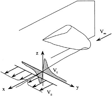
Fig. 1: Schematic of the way in which the velocity profiles, axial and tangential, are determined.
It should be pointed out that the vortex intensity obtained by adjusting the Lamb profile to the experimental and computational tangential velocity data is an arbitrary measure of a particularly ill defined property of the vortex. Indeed, since the circulation is defined as the integration along a closed path of the projection of the velocity vector over this path, if a closed path is selected around the tip vortex axis, the circulation of the velocity vector will increase continuously with the dimension of the path, since larger portion of the free vortex layer will be included within it. For a large enough path, the whole circulation of the wing will be reached. Because of this, the characteristic circulation of the tip has been selected in different ways by different authors. Moore [9] in his investigation of the rolling up of a discrete vortex distribution, considered that the circulation of the vortex at the extremity of the line was the sum of all vortices included in the spiral limited by an arbitrary vertical tangent. Shekarriz [10] integrated the maximum of the tangential velocity along a path coinciding with the position of this maximum. Fruman and co-workers have selected, as described above, the circulation which fits the tangential velocity profiles far from the core.
3 COMPUTATIONS
3.1 Mesh
The computational domain extends from one chord upstream of the leading edge point at mid-span to two
chords downstream the trailing edge at mid-span, Figure 2. These dimensions are based on a previous work conducted with STAR CD™ which shows that the lift coefficient is not further modified if the mesh is extended for more than two chords downstream.
The effect of the mesh refinement on the tip vortex is extremely important. Previous authors ([2]–[5]) stipulate that at least twenty cells are needed in the tip vortex viscous core in order to achieve mesh convergence. Since the trajectory of the tip vortex is a priori unknown, this geometric criterion is extremely difficult to satisfy directly without leading to a prohibitive number of cells. In order to circumvent this difficulty, a local refinement is realized on a set of cells determined from the results of a first calculation on a coarse mesh. As it will be explained later, the tip vortex core position and the extension to be refined are deduced directly from the pressure field.
The same coarse grid is used with both codes, STAR CD™ and FLUENT-UNS™, to avoid different results due to mesh effects. This grid is imported from STAR CD™ into FLUENT-UNS™ via a CAD platform.
3.2 Boundary conditions
The boundary conditions are indicated on Figure 2. We impose: a) at the inlet, a constant velocity distribution, b) on the walls and on the foil surface, a non-slipping condition, c) at the exit plane, a zero gradient condition called “outflow”.
Condition a) does not take into account the boundary layer which has develop upstream of the computational domain. The boundary layer thickness at the root of the foil is therefore under predicted, but this has probably only a very slight influence on the tip vortex development.
Condition b) is implemented via the use of wall functions. Those functions allow a finer grid on the walls but need to satisfy a dimensional criterion at the centroïd of the cells comprised between 10y+ and a 100y+, which is obtained by the modification of the mesh in an iterative manner. It should be noticed that this criterion has been applied and is satisfied only on the foil surface.
Condition c) is calculated in two stages. First, the distribution of variables at the exit plane are evaluated by extrapolation from the upstream, on the assumption of a zero diffusion flux for all variables ![]() except pressure. Then, the velocities are adjusted to satisfy the continuity equation. This condition permits to avoid the prescription of a pressure distribution which would need, as in Dacles-Mariani et al. [5], the use of a realistic pressure distribution based on experimental results. The computation would then become non-predictive.
except pressure. Then, the velocities are adjusted to satisfy the continuity equation. This condition permits to avoid the prescription of a pressure distribution which would need, as in Dacles-Mariani et al. [5], the use of a realistic pressure distribution based on experimental results. The computation would then become non-predictive.
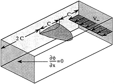
Fig. 2: Computational domain and boundary conditions at the inlet and outlet planes.
In order to test the influence of the boundary condition imposed at the outlet of the computational domain on the diffusion of the tip vortex, computations have been conducted with FLUENT-UNS™ in the following way. A first computation is carried out with the outlet boundary condition specified as above. Then, the pressure distribution on a plane normal to the free stream velocity situated at one chord downstream the tip is set as a boundary condition on the exit plane (at two and a half chord from the tip). This boundary condition is called “outlet pressure”.
3.3 Turbulence model
The inadequacy of turbulence models based on turbulent viscosity concept (Boussinesq [11]) for numerical tip vortex flows has been noticed by numerous investigators ([5], [12], [13]). Ziliac et al. [14] experiments have shown that in the tip vortex issued from a rectangular planform wing with a NACA 0012 cross section at a Reynolds of 4.6×10⁶, the Reynolds tensor is non-isotropic and is not aligned with the strain rate tensor. They conclude to the necessity of using non-linear k-ε (Speziale [15]) or second order (Zeman [16]) turbulence models. Actually, no second order turbulence models are available on STAR CD™. Calculations have been therefore conducted with three different turbulence models: the standard k-ε, the RNG k-ε and a non-linear k-ε model (Lien et al. [17]).
A k-ε RNG turbulence model and a second-order spatial discretization scheme is used with FLUENT-UNS™.
3.4 Numerical solution
The RANS equations are solved with a SIMPLE-type algorithm for pressure-velocity coupling. Three convection schemes have been used in this study. The
first, the UD scheme, is a first order upwind differencing scheme. The second one, QUICK, is a second order differencing scheme (see [18]). The third one is based on a multidimensional Total Variation Diminishing (TVD) scheme called MARS (Monotone Advection and Reconstruction Scheme). The calculation convergence criterion is based on the value of the normalized global residuals for all equations solved, apart the one for turbulence dissipation rate (see [19]).
Only calculations having normalized global residuals lower than 10−3 will be considered as converged.
3.5 Post-processing
The post-processing of the velocities is based on the same methodology than the one employed for the experiments. Thus, for a location downstream the tip, the position of the tip vortex center is first determined searching the minimum of the pressure field. This method is different from the experimental one based on velocity measurements, but preliminary tests have shown that, for the post processing of the numerical results, it is faster and more accurate. Then, the axial and tangential velocities are determined along the y axis for positions within 8 mm from the vortex center. The exact position of the vortex center which corresponds to the zero tangential velocity is then evaluated.
4 RESULTS AND DISCUSSION
4.1 Preliminary results
In order to evaluate the ability of the RANS codes to predict the flow in a correct way, the global hydrodynamic coefficients must be compared first. In Table 1 are presented the values of the lift coefficients obtained experimentally and by both codes with different turbulence models.
The mean of the turbulent numerical values is 0.573 with a maximum variation of + or − 2%. The “laminar” computation overestimates the lift coefficient, as compared to the mean of the turbulent, by 4%. All numerical results are always larger than measurements: the mean turbulent value is 6% larger than the experimental. Based on this global coefficient, it as clear that the FLUENT-UNS™ code with the k-ε RNG model gives the best result with an overestimation of only 4% of the experimental value. The difference between the experimental and the numerical values can be due to the fact that the secondary flow in the gap between the wing and the wall of the test section causes the reduction of the load at the mid span af the foil. The existance of this gap has not been accounted for in the computations.
Table 1: Lift coefficient comparisons.
|
Computation options |
Cℓ |
|
|
Experimental |
|
0.54 |
|
STAR-CD™ |
UD, laminar |
0.596 |
|
STAR-CD™ |
UD, non linear k-ε |
0.571 |
|
STAR-CD™ |
UD, k-ε RNG |
0.586 |
|
STAR-CD™ |
UD, k-ε |
0.574 |
|
FLUENT-UNS™ |
Quick, k-ε RNG |
0.562 |
The z and y position of the tip vortex center, obtained with the coarser mesh, using the STAR-CD™ code and the laminar, the k-ε, and the k-ε RNG models are plotted on Figure 3 together with the experimental results.
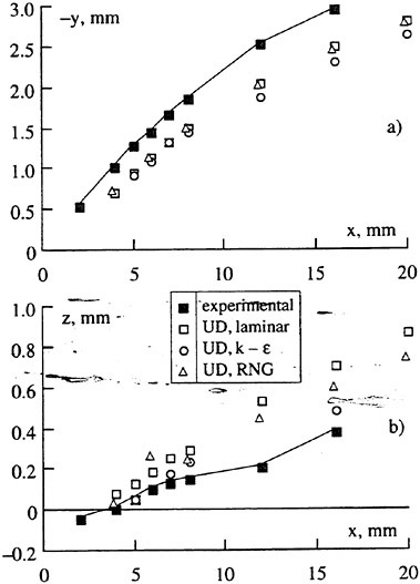
Fig. 3: Tip vortex trajectory path. Comparisons of the experimental results to the different numerical ones (initial mesh; laminar and k-ε calculations, STAR CD™).
The trend for the y position, representing the movement of the vortex towards the mid-span section, are very much the same. Taking into account the precision of the experimental and numerical results in determining the position of the vortex center, the agreement is rather good. In the vertical direction, for
which the displacements are smaller by nearly a factor of three, the trends are very good for a distance of less than 10 mm, one fourth of the maximum chord of the foil, but are over predicted afterwards. The position of the vortex center seems to be independent of the viscous effects since the laminar and the turbulent numerical results almost coincide everywhere, besides for the z position and x>10 mm. Figure 4 shows the tangential velocities measured and calculated for the same conditions as above at a station situated 4 mm (0.1 C) downstream the tip. In this very near region all computational results show maximum velocities well below the experimental values and larger vortex core dimensions. Moreover, the laminar calculation overpredicts significantly the velocity in the potential zone, while, whatever the turbulent model, the velocities at a distance of 2 mm outboard (0.05 C) coincide with the experimental results. The details in the core region are essential and desserve some attention. The position of the maximum for the k-ε RNG model is the closest to the one of the experimental results, but the value of the maximum is the smallest.
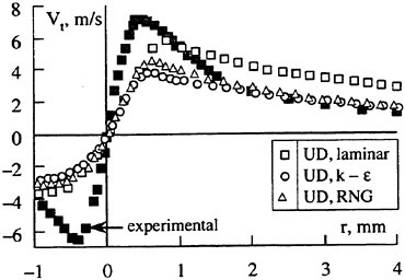
Fig. 4: Calculated (STAR CD™) and measured tangential velocities. Position downstream the tip: x/C=0.1.
It’s therefore obvious that, even in this very near region, the numerical results predict a core radius larger and a maximum tangential velocity lower than the experimental ones, thus an over diffused tip vortex. This over-diffusion is much more pronounced for a position 20 mm (0.5 C) downstream of the tip as it can be seen on Figure 5. Here, the maximum tangential velocity is about half and the core diameter is more than twice of the experimental results in the outboard region. In the inboard regions the velocities are flattened considerably and there is only a very slight indication of a minimum of the velocity for the laminar solution. There are marked changes in the case of the laminar computation in the outboard region since the velocities in the potential region approche now the predicted turbulent and experimental values. Therefore, numerical prediction of the tangential velocities deteriorates rapidly with distance downstream whatever the model and the region, either outboard or inboard.
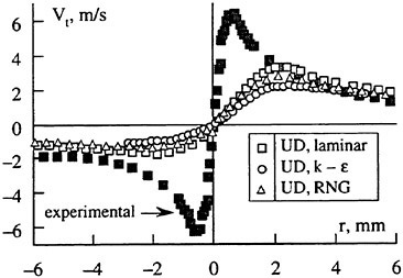
Fig. 5: Calculated (STAR CD™) and measured tangential velocities. Position downstream the tip: x/C=0.5.
Figure 6 and 7 show the axial velocities calculated and measured at 4 and 20 mm downstream the tip respectively. In the outboard region and at the closet station to the tip, the three numerical computations are very close; the k-ε RNG model predicting the largest axial velocity deficit. The velocity deficit is, at the most, larger than the experimental one by about 1 m/s (0.1 of the free stream velocity). The deficit is initiated at a distance from the axis comparable to the one at which the corresponding tangential velocities leave the potential region.
Farther downstream the changes are significant, The velocity deficit is sharply reduced in the numerical computations while the experimental one increases. In the outboard region for a radial distance larger than about 3 mm (0.075 C) and in the inboard region the numerical and experimental results nearly coincide. However, a marked experimental velocity overshoot within the core is ignored by the computations.
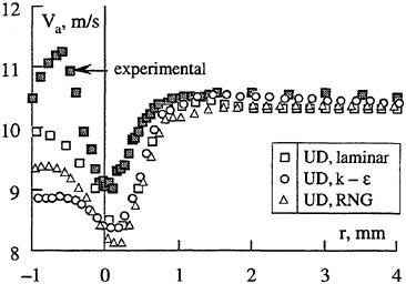
Fig. 6: Calculated (STAR CD™) and measured axial velocities. Position downstream the tip: x/C=0.1.
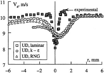
Fig. 7: Calculated (STAR CD™) and measured axial velocities. Position downstream the tip: x/C=0.5.
In Figure 8 we have plotted the core radius divided by the thickness of the turbulent boundary layer, δ, computed as for a flat plate of length equal to the midspan chord, C,
where ν is the kinematic viscosity. The over-diffusion is clearly shown, the numerical core radius at the stations just downstream the tip being larger and growing faster than the experimental ones whatever the model used in the computations. At a distance of 0.5 C the numerical predictions are twice the ones issued from the experiments.
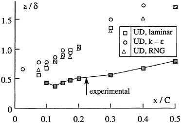
Fig. 8: Non dimensional local core radius versus distance downstream of the tip. Numerical (STAR CD™) and experimental values.
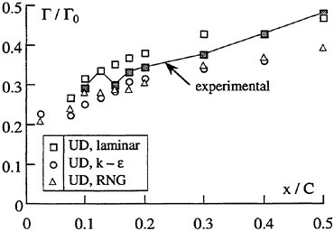
Fig. 9: Non dimensional local vortex intensity versus distance downstream of the tip. Numerical (STAR CD™) and experimental values
Figure 9 shows the vortex intensity divided by the mid span foil circulation, Γ0,
where C and Cℓ are respectively the mid span chord and the lift coefficient. The numerical prediction are in general good agreement with the experimental ones. It should be pointed out, however, that the “laminar” results slightly over evaluated while the turbulent ones are under evaluated.
4.2 Effects of the mesh refinement
The refinement methodology used is based on a pressure criterion. Once an initial calculation, let us
say the “laminar” one, has been made, the pressure distribution can be obtained as exemplified in Figure 10 where the tangential velocity profile has been also plotted for a position located 4 mm downstream the tip. It is clear that 90% of the pressure drop, P∞−P0 is within a distance of slightly more than 2 mm, or twice the viscous core dimension defined as the position of the maximum of the tangential velocity.
The set of cells where the pressure is lower than the level Plc are selected for mesh refinement, each cell is divided in half its each size with a total number of cells increasing from 280,000 for the coarse mesh to 350,000 for the refined mesh.
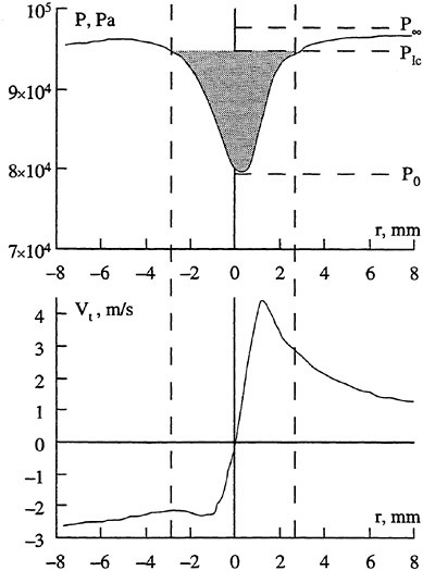
Fig. 10: Illustration of the set of cells selection process.
Figure 11 reproduces the results of Figure 9 and adds those obtained with the refined mesh. The refinement has no influence on laminar and k-ε calculations and slightly decreases the intensity for the k-ε RNG calculation.
The effect of the mesh refinement on the core radius evolution is shown in Figure 12. At the closest station from the tip (0.025 C) the laminar calculation with the refined mesh decreases very significantly the core radius while the k-ε RNG increases it as compared with the result obtained with the k-ε model and the initial coarse mesh. Downstream this station the effect of the mesh refinement is not as spectacular and corresponds to a moderate decrease of the predictions made with the coarse mesh. We are still far from the experimental predictions of the core radius and improving the mesh refinement seems to be of limited value to fill the remaining gap. Let us see next how other changes improve the results.
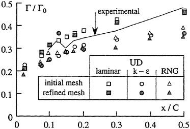
Fig. 11: Non dimensional local vortex intensity versus distance downstream of the tip. Numerical (STAR CD™) and experimental values. Effect of mesh refinement.
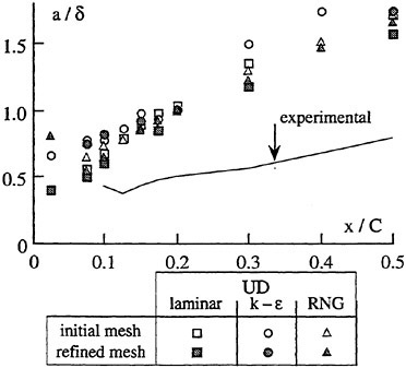
Fig. 12: Non dimensional local core radius versus distance downstream of the tip. Numerical (STAR CD™) and experimental values. Effect of mesh refinement.
4.3 Effect of the turbulence model
The effect of the three turbulence models (k-ε, k-ε RNG and k-ε non-linear) was analyzed using the coarse
grid and the first-order scheme (UD). The non linear k-ε model causes the increase of the local vortex intensity as compared to the other two turbulence models. This can hardly be explained since the vortex intensity is essentially determined by the roll-up of the potential flow, unaffected by the turbulence prevailing in the core. In spite of the increase of the vortex intensity, the results fall below the experimental ones in the region comprised between 0.3 and 0.5 C.
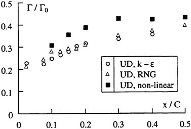
Fig. 13: Non dimensional local vortex intensity versus distance downstream of the tip. Numerical (STAR CD™) and experimental values. Effect of turbulence model.
It can be seen on Figure 14 that the k-ε RNG or the non-linear k-ε models slightly decrease the size of the core radius as compared to the k-ε. It was expected that the non-linear k-ε model would improve the results and decrease considerably the vortex core dimension. The obtained predictions may be due to the lack of accuracy of the UD scheme, which has to be replaced with a second-order discretization scheme.
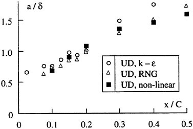
Fig. 14: Non dimensional local core radius versus distance downstream of the tip. Numerical (STAR CD™) and experimental values. Effect of turbulence model.
4.4 Effect of the convection scheme
The effect of the numerical scheme has been analyzed through calculations in the “laminar” regime with the coarse mesh and two schemes, namely UD and MARS. As shown in Figure 15, the numerical scheme has a slight influence on the non dimensional local intensity.
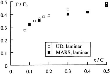
Fig. 15: Non dimensional local vortex intensity versus distance downstream of the tip. Numerical (STAR CD™) and experimental values. Effect of the numerical scheme.
Figure 16 shows that, on the contrary, the use of the MARS scheme decreases significantly the non dimensional core radius. Therefore, in the non turbulent conditions, the numerical scheme affects significantly the core size but does not changes the vortex intensity.
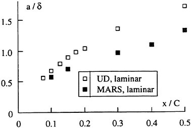
Fig. 16: Non dimensional local core radius versus distance downstream of the tip. Numerical (STAR CD™) and experimental values. Effect of the numerical scheme.
4.5 Effect of the exit boundary condition (computations with FLUENT-UNS™)
The aim of this approach is to test the influence of the boundary condition imposed at the exit of the computational domain on the diffusion of the flow downstream the hydrofoil.
The tangential velocity profiles obtained at x/C=0.1 and x/C=0.5 with both exit boundary conditions are shown on Figures 17 and 18. At the position closest to the tip the results of the FLUENT-UNS™ code are better than the ones obtained with STAR-CD™ whatever the boundary condition in the exit plane of the computational domain. However, this improvement does not last because at the position half a chord downstream the maximum velocities have decreased and the vortex core increased considerably. The results remain however better than those obtained with STAR-CD™. The prediction of the tangential velocity gradients obtained by FLUENT-UNS™, as compared to the other RANS codes, show the excess of diffusion of the tip vortex. This diffusion is probably due to the turbulence model and to the convection scheme which one leads to a numerical diffusion. On Figure 19 and 20 the axial velocities at two stations, x/C=0.1 and x/C=0.5, obtained with both exit boundary conditions are shown. In the outboard region, the results are very close together regardless of the boundary condition imposed at the exit of the domain. At 0.1 chord from the tip the velocity deficit on the vortex axis is larger than the experimental one and even larger than the one predicted at the same station by STAR-CD™. At 0.5 chord from the tip the results are remarkably close to the experimental results in the outboard region besides for the fact that the experimental velocity overshoot is not represented.
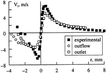
Fig. 17: Calculated (FLUENT-UNS™) and measured tangential velocities. Position downstream the tip: x/C=0.1.
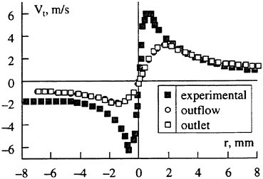
Fig. 18: Calculated (FLUENT-UNS™) and measured tangential velocities. Position downstream the tip: x/C=0.5.
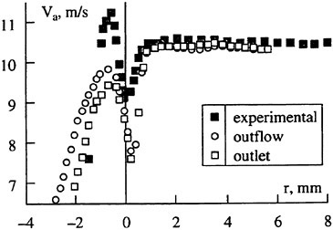
Fig. 19: Calculated (FLUENT-UNS™) and measured axial velocities. Position downstream the tip: x/C=0.1.
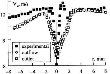
Fig. 20: Calculated (FLUENT-UNS™) and measured axial velocities. Position downstream the tip: x/C=0.5.
In order to evaluate the impact of the exit boundary condition on the diffusion, the tangential velocity, the axial velocity and the static pressure profiles are shown at five stations between the tip and 2,25 chord, very close to the exit of the computational domain.
In Figure 21 it can be seen that the effect of the boundary condition on the tangential velocity profiles is hardly distinguishable everywhere besides for the farther downstream station where the tangential velocity gradient through the viscous core is slightly increased by the “outlet condition”.
The axial velocities, Figure 22, are also very lightly modified by the “outlet pressure” condition if the results in the outboard region are considered first. In the inboard region, where the influence of the hydrofoil is the most important and at x/C=0.1 the differences are significant. The static pressure profiles through the tip vortex, shown on Figure 23, are very slightly disturbed by this change of the condition at the exit. This is not surprising taking into account the changes observed in the velocity profiles.
Finally, the tested boundary conditions at the exit of the flow domain have a minor influence on the tip vortex development and a negligible one on the pressure distribution. The poor representation of the tangential velocities in the core region persists while the axial velocities are in better agreement with the experiments.
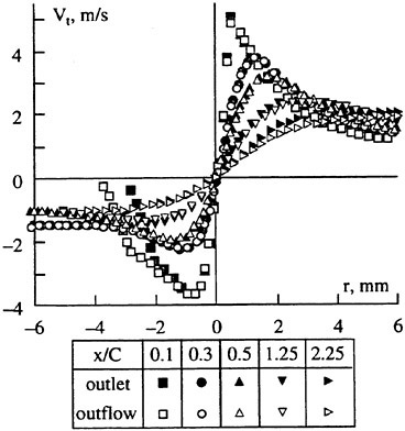
Fig. 21: Tangential velocity distributions for different positions downstream the tip. Influence of the exit boundary condition.
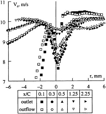
Fig. 22: Axial velocity distributions for different positions downstream the tip. Influence of the exit boundary condition.
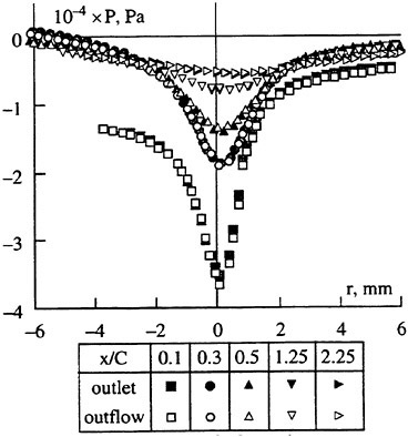
Fig. 23: Influence of the exit boundary condition on the static pressure.
4.6 Pressure coefficient
In Figure 24 we have plotted the pressure coefficient,
directly predicted by the numerical approach and the one estimated using the expression,
where Γ and a are obtained by fitting the Lamb velocity profile to the tangential velocities profiles issued from the numerical computation.
It is very interesting to note that: a) the evolution of the pressure coefficients follows the same trend whatever the way they are computed, and b) the predictions given by the simplified method of using the limited tangential velocity data, Cp0Lamb, are generally lower than those obtained from the full pressure field. Moreover, the computations conducted using the MARS scheme and a non linear k-ε model are the closest to the experimental results. A pressure minimum occurs at a distance of less than one tenth of the foil chord, as predicted experimentally.
Thus, the methodology used by the ACC partners to evaluate the pressure on the vortex core using the experimental tangential velocity profile obtained along a line parallel to the foil span seems to be fully justified by the numerical results, even if the absolute values are not in close agreement.
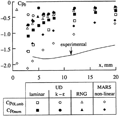
Fig. 24: Pressure coefficient on the vortex axis as a function of the distance to the tip. Effect of the method of estimation of the pressure coefficient.
5 CONCLUSION
Computation of the flow field around an elliptical planform hydrofoil was conducted using two RANS codes, STAR CD™ and FLUENT-UNS™. The results were compared between them and with experimental results.
The conclusions can be summarized as follows:
-
the agreement between the numerically and experimentally predicted non dimensional local vortex intensities along the vortex path is very good whatever the computation. The potential flow is thus correctly represented by the codes.
-
the local vortex core radii are systematically over estimated by the both RANS codes and, therefore, the pressure on the vortex axis is under estimated. The flow in the viscous region is not correctly predicted.
The effect of modifications of the grid, by refining it on a region confined to the vortex core, of the turbulence model and of the boundary condition at the exit of the computational domain was investigated. It appear that:
-
the grid refinement has a relatively low influence on the local vortex intensity and slightly decreases the local vortex core radius;
-
the use of a k-ε RNG or non linear k-ε model decreases the local core radius as compared to the k-ε model;
-
the higher order discretization scheme strongly decreases the local core radius as compared to the first order scheme;
-
the exit pressure condition has a very slight effect on the tangential velocity distribution in the core, but a slightly larger one on the axial velocity distribution.
The numerical computation results have allowed to show that the methodology used by the ACC partners to evaluate the pressure on the vortex core using the experimental tangential velocity profile obtained along a line parallel to the foil span seems to be fully justified, even if the absolute values are not in close agreement.
The over prediction of the vortex diffusion by all numerical codes, commercial or specifically developed, whatever the “receipt” utilized to improve the results, is by now fully demonstrated. Major breakthroughs need to be achieved if this essential academic and industrial problem is to be resolved.
ACKNOWLEDGEMENTS
The authors are grateful to the “Direction des Recherches, Etudes et Techniques (DRET) du Ministère Français de la Défense” for its support. This
work was conducted within the scientific program of the “Action Concertée Cavitation (ACC)”.
REFERENCES
[1] Freitas C.J., “Numerical study of the tip vortex flow over a finite span hydrofoil”, FED-Vol. 238, 1996, Fluids Engineering Division Conference, Volume 3, pp. 65–74.
[2] Dupont P., Hirschi R., Billard J.Y., “Prédiction de la cavitation liée à l’enroulement en extrémité d’un hydrofoil de forme en plan elliptique”.—La Houille Blanche, 1997, n° 4/5
[3] Deniset F., “Modélisation numérique des conditions d’apparition de la cavitation de tourbillon marginal sur une aile-3D. Effet de confinement”, Thèse de l’Institut National Polytechnique de Grenoble, June 1996.
[4] Eça L., Falcao de Campos J., Hoekstra M., “Prediction of incompressible tip vortex flows”, Twentieth Symposium on Naval Hydrodynamics, August 1994, Santa Barbara, California, pp. 17–31.
[5] Dacles-Mariani J., Zilliac G.G., Chow J.S., Bradshaw P., “Numerical/Experimental study of a wingtip vortex in the near field”, AIAA Journal, vol. 33, No. 9, Sept. 1995, pp. 1561–1568.
[6] Viot X., “Cavitation de tourbillon marginal, effet du fractionnement de l’aile”, Thèse de l’Université Paris 6, April 1998.
[7] Fruman D.H., “Recent progress in the understanding and prediction of tip vortex cavitation”, 2nd International Symposium on Cavitation, 1994, Tokyo, Japan, Proc. H.Kato ed., pp. 19–29.
[8] Fruman D.H., “The Action Concertée Cavitation research program and accomplishments”, International Symposium on Cavitation, CAV’95, May 1995, Deauville, pp. 211–217.
[9] Moore D.W., “A numerical study of the roll-up of a finite vortex sheet”, JFM, 1974, vol. 63, pp. 225–235.
[10] Shekarriz A., Fu T.C., Katz J., Huang T.T, “Near-field behavior of a tip vortex”, AIAA Journal, vol 31, n° 1, pp. 112–118, 1993.
[11] Boussinesq J, “Théorie des écoulements tourbillonnaires”, Compte Rendu de l’Académie des Sciences, 1877, Tome 23.
[12] Dacles-Mariani J., Rogers S., Kwak D., Zilliac G., Chow J., “A computational study of wingtip vortex flow field”, AIAA 24th Fluid Dynamics Conference, July 1993, Orlando.
[13] Hsiao C.T., Pauley L.L., “Numerical study of the tip vortex flow over a finite span hydrofoil”, FED-Vol. 238, 1996 Fluids Engineering Division Conference, Volume 3, pp. 65–74.
[14] Zilliac G.G., Chow J.S., Dacles-Mariani J., Bradshaw P., “Turbulent structure of a wingtip vortex in the near field”, AIAA 24th Fluid Dynamics Conference, July 1993, Orlando.
[15] Speziale C.G., “On non-linear K-l and K-ε models of turbulence”, JFM, 1987, vol. 178, pp. 459–475.
[16] Zeman O., “The persistence of trailing vortices: a modelling study”, Phys. Fluids 7(1), January 1995, pp. 135–143.
[17] Lien F.S., Chen W.L., Leschziner M.A., “Low-Reynolds Number eddy-viscosity modelling based on non-linear stress-strain/vorticity relations”, Proc. 3rd Symp. on Engineering Turbulence Modelling and Measurements, May 1996, Crete, Greece.
[18] Ferziger J.H., Peric M., “Computational methods for Fluid Dynamics”, Springer editions.
[19] STAR CD Users Manual Version 3.0
DISCUSSION
Η.Raven
Maritime Research Institute, The Netherlands
This interesting paper clearly shows the difficulty of resolving this complicated flow numerically. For example, Fig. 16 indicates a large difference in the results with various different schemes. The upward scheme most likely introduces a large numerical viscosity, apparently much larger than the differences in eddy viscosity between turbulence models (Fig. 14). Are not, then, the conclusions on the effect of the turbulence model on the results somewhat premature?
AUTHORS’ REPLY
The comparison of Figure 14 and 16 seems to indicate that the first-order upwind scheme introduces a large numerical viscosity, much larger than those introduced by the turbulence models themselves. Because of calculation convergence problems, we didn’t have results with a second-order scheme and with the three different turbulence models which would allow us to conclude unequivocally on the effect of the turbulence model. Indeed, the use of a non-linear turbulence model with a higher order discretization scheme simulta-neously should strongly improve the results, particularly the prediction of the tip vortex core radius.
DISCUSSION
M.Billet
Applied Research Laboratory, USA
The scientific program of the “Action Concertee Cavitation” into the physics of tip vortices roll-up has provided significant insight to the cavitation and propeller design communities. The authors are to be congratulated for their research, which was a coordinated experimental and computational program. This paper discusses some of the numerical results and it is very encouraging that the methodology used to analyze the experimental data is supported by the numerical results. However, rather large differences exist between the experi-mental and numerical results. This, we propose, is due in large part to the ability of the “available” codes to predict the flowfield.
The mesh refinement study conducted in this investigation is not sufficient to conclude that a mesh independent solution was achieved. At least three levels of grid resolution are required to make a valid grid error assessment. Also, the first-order upwind differencing (UD) scheme is not adequate. Higher order schemes are a necessity for problems such as this, unless a truly mesh independent solution has been achieved. Have the authors conducted any additional grid studies that clarify the question of grid and differencing (other than the MARS results) errors?
The details of the vortex formation process are dependent on tip geometry and viscous effects, while the overall process is driven by the loading difference between the suction side and pressure side of the foil. It is likely that the question of foil near-wall resolution is important, and the use of wall function boundary conditions on the foil may not properly simulate the tip vortex formation. Have the authors investigated near-wall resolution effects on the tip vortex formation and near-tip structure?
The authors stated that the agreement between their predictions and experimental data were “rather good.” This statement is too subjective. A more detailed quantification of the differences is warranted including uncertainty analysis of both the experimental results and the computations.
The authors’ conclusion that all codes overpredict vortex diffusion is probably correct. The reasons are likely inadequate grid resolution in some cases and the inability of commonly used turbulence models to model the vortex diffusion processes in all cases.
AUTHORS’ REPLY
First, the authors thank Michael L.Billet and Howard J.Gibeling for their congratulations about this work, conducted on the basis of the numerous results obtained by the scientific program of the “Action Concertée Cavitation.”
Mesh refinement:
The refinement tests conducted in this work show that the vortex intensity and the local core radius are slightly sensitive to the increase of the spatial resolution in the tip region.
The aim of our work was not to conduct a complete mesh refinement study; only the effect of a local (i.e., on the tip vortex path) refinement, based on the pressure level in the tip vortex core, has been investigated. However, it should be noticed that the initial mesh results from previous investigations have shown a mesh convergence on the foil pressure distribution.
Near-wall resolution:
It hasn’t been possible to conduct calculations with a near wall resolution (i.e., with two-layer models) on the foil. However, if one considers the near tip value of nondimensional local core radius and vortex intensity (see Fig. 8 and 9), it should be expected that the tip vortex formation is quite well predicted. Effectively, the statement that the agreement between our prediction and experimental data is rather good is somehow subjective and means that the agreement is qualitatively good.
General observation and uncertainty analysis:
The uncertainty analysis of the experimental tip vortex velocity is a very difficult task because of the intrinsic bias due to the finite measuring volume and to the vortex wandering. It is by now well known that the consequence of this bias leads to an underestimation of the maximal tangential velocity and an overprediction of the core radius (Pauchet et al. [1]). A recent work [2] on the effects of turbulence and wandering on tip vortex development has been conducted at the L.H.E.N. (Laboratoire d’Hydrodynamique de l’Ecole Navale).
DISCUSSION
J.Dacles-Mariani
NASA Ames Research Center, USA
The authors mentioned some compelling reasons for the difficulties associated with predicting the tip vortex flow accurately. Here are some specific comments:
Mesh Refinement:
1. Tip vortex flow is an evolving process; you cannot expect to obtain good comparison downstream if you are not resolving it as it is being formed on the surface. Some grid refinement study to determine where you will need to refine the grid locally, (resolving the high gradients, etc.), will have to be done before one can get good results. The number of grid points across the viscous vortex core of at least 20 only applies when the vortex has been formed in the near-wake. When the vortex is still forming, this may not be the case.
2. The trajectory of the vortex is not known a priori and so it makes sense to do trial runs using a coarse grid to determine where the vortex lies first before refining the grid. (This was also implemented by Dacles-Mariani et al., 1995.)
Convection Scheme:
Our study showed a different behavior. We did the initial study on an analytical vortex (3-D Burgers Vortex) and found that there is a significant improvement by going from 3rd-order to the 5th-order upwind-biased differencing.
Turbulence Model:
We found that one-equation turbulence models overpredict the eddy viscosity at the core. We had applied a modification to empirically adjust the production term and thus in turn reduce the artificial viscosity coming from the turbulence model.
General Comment:
1. There is a difference in the way the vortex core is being underpredicted/overpredicted between Viot et al. and our work. In our study, using 2.5 million grid points, the velocity profiles compare well with measured data, but the static pressure is overpredicted only in the viscous region of the vortex core. This is different from their results showing a general “smearing” of the whole vortex core. Do the authors have any comments on this?
2. It wasn’t clear in their paper if the experiment also showed an axisymmetric vortex profile at 2 chords downstream; that is, is the measured vortex really axisymmetric at this location?
3. A recent study by Dacles-Mariani et al. (1993, 1996) addressed most of these issues. They attempted to isolate the roles of numerics and turbulence modeling in accurately predicting the tip vortex flow. The approach they took relied heavily on some detailed experimental results and incorporated them in the computation as inflow and outflow
boundary conditions. Although this procedure is not duplicatable, it was valuable in helping to establish some guidelines in resolving tip vortex flows. This was the sole intent of their study. They recognized that before one can obtain some accurate tip vortex simulation, a detailed study to quantify to some extent the roles of numerics and turbulence modeling was needed. (See Figs, 1a and 1b which are the results from implementing the guidelines we found from our work using 2.5 million grid points.)
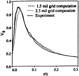
Fig. 1a Effective crossflow velocity profile.
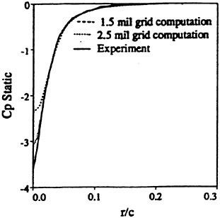
Fig. 1b Static pressure coefficient profile.
Fig. 1 Comparison of flow quantities in the wake region at x/c=1.462 for two grid sizes using Spalart-Allmaras one-equation model. (Dacles-Mariani et al, 1996).
AUTHORS’ REPLY
Mesh refinement:
In this work, a new mesh refinement technique based on the pressure level in the tip vortex core has been tested. Other tests have to be conducted, particularly close to the foil surface, in order to determine in a better way the regions where the spatial resolution has to be strongly improved.
The grid used in this work was obtained after several computations conducting from the initial grid to the final one. This methodology has permitted precise determination of the position of the tip vortex trajectory.
Convection scheme:
The use of a high order discretization scheme improves the prediction of the local tip vortex core radius but has a very slight effect on the prediction of the local vortex intensity. It should be expected that a higher order discretization scheme should improve the results.
Turbulence model:
The nonlinear turbulence model improves the prediction of the tip vortex core radius. This is due to a better estimation of the viscosity used by the model in this region than with the k-ε model.
General comment:
1. As the experimental static pressure is calculated by using the experimental velocity and the radial equilibrium law, it would be surprising, in our case, to have a very good agreement for the experimental velocity and an overprediction of the static pressure as in the study of Dacles-Mariani et al.
2. Yes, the experiment shows an axisymmetric vortex profile at two chords downstream.
3. In a similar way to Dacles-Mariani et al., our aim was to isolate the roles of different paramaters such as turbulence model, numerical scheme, mesh refinement, and boundary conditions. That’s why, in our investigations, only one parameter has been changed at one time.
Prediction of Propeller Blade Sheet and Developed Tip Vortex Cavitation
S.Kinnas, H.Lee, A.Mueller (University of Texas at Austin, USA)
ABSTRACT
A potential based panel method for the prediction of unsteady sheet cavitation on hydrofoils or propeller blades, is extended to include (a) the effects of a general cross-section tunnel, (b) the modeling of face leading edge or mid-chord sheet cavitation, and (c) the modeling of a developed tip vortex cavity.
1 INTRODUCTION
Prediction of blade sheet cavitation and its induced pressure field on the hull is very critical in the assessment of propulsor designs. Modern naval or commercial propulsor blades tend to produce “flat” wetted flow pressure distributions on the suction side which may lead to the presence of either bubble or mid-chord sheet cavitation [8]. In addition, unloading the blade tip in order to avoid tip vortex cavitation is practically impossible, in particular since most propulsors operate inside non-axisymmetric wakes. Thus, the presence of a developed tip vortex cavity (often connected to the blade sheet cavity) is very common. The prediction of the shape of the tip vortex cavity and its variation with blade angle have been found to be critical in determining the propeller induced hull pressures.
Boundary element methods for the prediction of unsteady sheet cavitation in non-linear theory have already been developed [9, 11, 10]. The effects of viscosity were added in the above methods via an integral boundary layer approach [12]. The methods were validated versus a cavitating hydrofoil experiment in 2-D [1] and more recently versus a 3-D cavitating propeller experiment, named CAPREXII [14] with the effects of the tunnel walls being included via direct modeling with a panel method [2, 16]. Photographs of the observed cavities are shown for various blade angles at the top part of Figure 1 while the predictions at the corresponding blade angles are shown at the bottom part of the same figure. Note in the
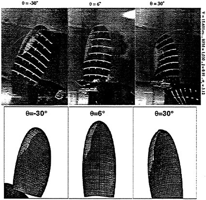
Figure 1: Blade cavitation as observed in CAPREX II (top) and predicted by a panel method (bottom).
photographs the presence of a developed tip vortex cavity and its attachment (in some cases) with the blade cavity. Note also the failure of the prediction method to capture the cavity shape at the tip of the blade.
In this work, a boundary element method is extended to model the effects of face cavitation, tunnel walls, as well as the flow in the region of a developed tip vortex cavity.
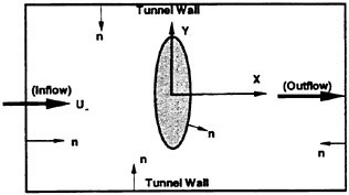
Figure 2: A 3-D hydrofoil inside of a tunnel, and their images used in the numerical model. The top half of the hydrofoil is mounted vertically on the tunnel bottom wall, which is located in between the two shown walls.
1 Cavitating hydrofoil inside a tunnel
1.1 Formulation
Consider a 3-D cavitating/non-cavitating hydrofoil inside a tunnel, as shown in Figure 2. The physical problem corresponds to the top half of the shown hydrofoil being mounted on the bottom (flat) wall of a tunnel with cross section that of the top half shown in the figure. The effect of the tunnel walls has already been included in the case of 2-D hydrofoils and cavitating propellers inside of rectangular tunnels, by modeling the tunnel walls via a low-order boundary element method [3, 2].
The normal unit vector, ![]() is defined as positive when pointing towards the fluid domain. The origin of the XYZ-coordinate system is located at the center of the hydrofoil, the positive X direction is defined towards downstream and the positive Υ direction is toward the tip of the hydrofoil. The lengths are made non-dimensional with respect to the actual span of the real hydrofoil1
is defined as positive when pointing towards the fluid domain. The origin of the XYZ-coordinate system is located at the center of the hydrofoil, the positive X direction is defined towards downstream and the positive Υ direction is toward the tip of the hydrofoil. The lengths are made non-dimensional with respect to the actual span of the real hydrofoil1
The governing equation everywhere inside the fluid domain is given as.
(1)
where ![]() is the perturbation potential defined as follows;
is the perturbation potential defined as follows;
(2)
|
1 |
In this work, we call “radius” the actual span of the foil, and “diameter” the span of the double hydrofoil, i.e. foil and image. |
where ![]() is the total velocity vector and
is the total velocity vector and ![]() the inflow velocity vector.
the inflow velocity vector.
By applying the Green’s third identity to the governing equation (1) in the fluid domain, as shown in Figure 2, we get the following integral equation for the perturbation potential on the hydrofoil or tunnel wall surfaces
(3)
where ST, SH and SW are the boundaries of tunnel wall, hydrofoil and wake.
Equation 3 can be solved by applying a BEM on all involved surfaces simultaneously. In the present case we have applied an iterative method similar to that presented in [3]. In this method the problem is actually solved either on the hydrofoil or on the tunnel while the interaction is taken into account iteratively.
We first define the potential in the flow domain due only to the influence of the tunnel ![]() or of the hydrofoil
or of the hydrofoil ![]() :
:
(4)
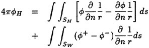
(5)
where ![]() is the induced potential on the hydrofoil surfaces due to the tunnel wall, and
is the induced potential on the hydrofoil surfaces due to the tunnel wall, and ![]() is the induced potential on the tunnel boundaries due to the hydrofoil.
is the induced potential on the tunnel boundaries due to the hydrofoil.
By substituting equation (4) into equation (3), we can get an integral equation for the external flow around the hydrofoil:
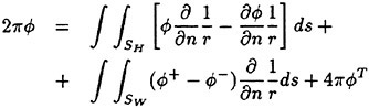
(6)
and, similarly an integral equation for the internal flow inside the tunnel:
(7)
Integral equations (6) and (7) are solved successively via a low-order boundary element method [3],
with the terms ![]() and
and ![]() being updated during the iterative process. The main difference of the present method from that of [3] is that the hydrofoil “feels” the tunnel via its potential field as opposed to via its velocity field.
being updated during the iterative process. The main difference of the present method from that of [3] is that the hydrofoil “feels” the tunnel via its potential field as opposed to via its velocity field.
In addition, the following boundary conditions need to be applied:
On the hydrofoil
To get a uniquely determined potential, ![]() , around the cavitating hydrofoil, the following boundary conditions are imposed [11]:
, around the cavitating hydrofoil, the following boundary conditions are imposed [11]:
-
The flow tangency condition on the foil surface: the fluid flow is tangent to the hydrofoil surfaces.
(8)
-
The kinematic condition on the cavity surface
(9)
where F(x, y, z) is a function expressing the cavity surface and
 is the cavity velocity.
 -
The dynamic condition on the cavity surface: the pressure on the cavity surface is equal to the vapor pressure,

(10)
or
(11)
where pν is the vapor pressure, qc the magnitude of the cavity velocity, and σ the cavitation number defined as usual:
(12)
-
The Kutta condition: the velocity at the trailing edge of the hydrofoil is finite.

(13)
-
The cavity closure condition: the cavity thickness at the cavity end should be equal zero.
On the tunnel walls
Assuming that the tunnel walls are fixed and the flow is coming from far upstream with uniform velocity, U∞, the following conditions apply:
-
On the solid wall boundaries: the fluid flow normal to the solid walls is equal to zero.

(14)
-
At the inflow and outflow boundaries: the total velocity normal to the in/out boundaries is equal to the uniform flow;

(15)

(16)
1.2 Validation and results
1.2.1 Non-cavitating hydrofoil
The described numerical scheme is first applied on a non-cavitating hydrofoil. A 3-D hydrofoil with an elliptic planform is used. The thickness to chord ratio is 6%, the chord to diameter ratio is 17%, and the angle of attack α=4°. This hydrofoil also has a linear twist distribution along the span with 0° at the base of the hydrofoil and −4° at the tip. The tunnel width to hydrofoil diameter ratio is equal to 2. The (actual) tunnel height to hydrofoil diameter ratio is equal to 1.
Figure 3 shows the pressure convergence characteristics for each iteration, at y=0.04 and y=0.485 on the hydrofoil. The pressure distribution from the first iteration corresponds to that without the tunnel effects. Note the quick convergence with number of iterations.
Figure 4 shows the variation in the lift coefficient of the hydrofoil due to the effect of the tunnel width to the hydrofoil diameter ratio. The blockage effect on the hydrofoil surface due to the tunnel walls is negligible for tunnel width to hydrofoil diameter ratio larger than two. Figure 5 shows the effect of the tunnel width on the spanwise circulation distribution on the hydrofoil.
1.2.2 The cavitating 4990 hydrofoil
The method is applied on the 4990 hydrofoil the geometric characteristics of which are given in Appendix A. A cavitation test for this hydrofoil was conducted at the DTMB 36 inch cavitation tunnel. This hydrofoil was designed to have the same planform and loading as the blades of the DTMB N4990 propeller
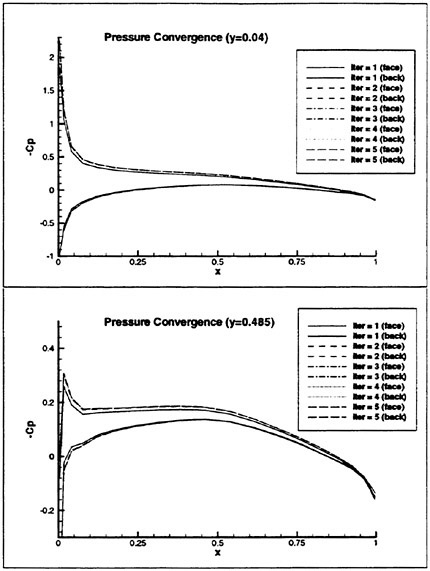
Figure 3: The pressure convergence history at y=0.04 and y=0.485 on the hydrofoil. Elliptic foil at angle of attack α=4° with twist angle of 4° (opposite to α) at the tip, 6% thickness to chord ratio, 17% chord to diameter ratio. The width of the tunnel to hydrofoil diameter ratio is equal to 2. The (actual) height is equal to the hydrofoil diameter.
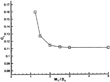
Figure 4: Effect of tunnel width to foil diameter ratio on the lift coefficient. Same foil and conditions as in the previous figure.
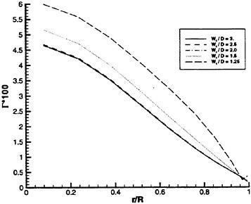
Figure 5: Effect of tunnel width to foil diameter ratio on the lift coefficient. Same foil and conditions as in the previous figure.
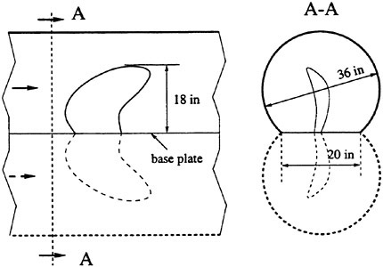
Figure 6: Schematic of the 4990 hydrofoil inside the DTMB 36” circular section tunnel. Also shown is the image of the hydrofoil and tunnel as employed in the numerical model.
at design conditions [7]. A photograph from the experiment is shown in Figure 10. A schematic of the setup is shown in Figure 6. The (actual) span of the hydrofoil is equal to 18 inches while its maximum chord is 24.4 inches. The 4990 hydrofoil was mounted vertically at an angle of attack of α=0°.
The used numerical grids on the hydrofoil and the tunnel walls are shown in Figure 7. The hydrofoil and the part of the circular tunnel above the mounting plate are imaged with respect to the plate so that the kinematic boundary condition is automatically satisfied on the plate surface. Figure 8 shows the convergence history of the hydrofoil circulation with number of iterations between the tunnel and the hydrofoil. Note that almost the complete tunnel effect has been “felt” by the foil at the end of the second iteration.
Predicted cavity shapes, with and without the tunnel effects included, are shown in Figure 9. Note the drastic effect of the tunnel walls on the predicted cavity shape. The predicted cavity planform when the tunnel effects are included appears to be very close to the observed, shown in Figure 10. However, there are flow phenomena at the root of the blade (re-entrant jet, cloud cavitation at the trailing edge) which are not modeled in the present method and thus not captured by the predictions.
Finally, the drastic effect of the cavity detachment location on the predicted cavity shape for the 4990 hydrofoil is demonstrated in Figure 11. The cavity shapes and planforms shown in Figure 11 have been predicted in unbounded flow but with the 4990 hydrofoil at an angle of attack of α=1.3°, which produces about the same loading to that of the 4990 hydrofoil (at α=0°) inside the tunnel. The predicted cavity with the tunnel effects included, as shown in Figure 9, has been determined by manually adjusting the cavity leading edge at each section along the span until two conditions are satisfied: (a) the cavity thickness is positive and (b) the pressures upstream of the cavity detachment are larger than the vapor pressure.
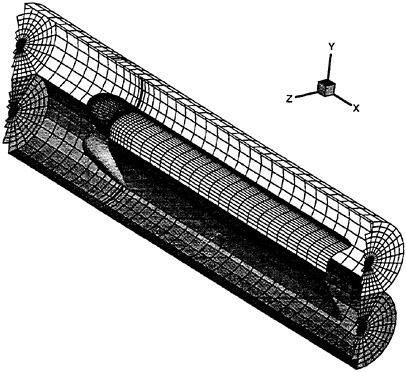
Figure 7: The grid on the 4990 hydrofoil, its trailing wake, and the DTMB 36” circular tunnel (the images are also shown). Only the outer part of the tunnel panels are displayed.
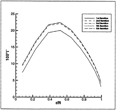
Figure 8: Convergence history for the circulation over the 4990 hydrofoil with number of iterations between the tunnel and the hydrofoil solution (the 1st iteration corresponds to the unbounded flow); α=0°, non-cavitating flow.
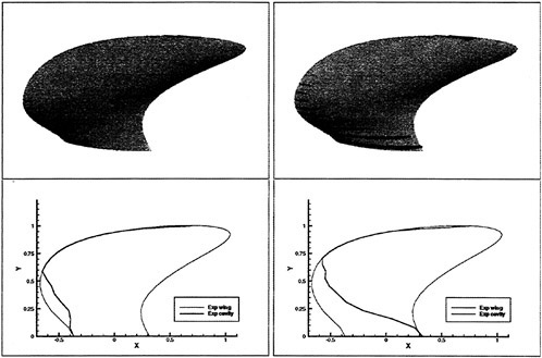
Figure 9: The predicted perspective (top) and expanded (bottom) cavity planforms without (left) and with (right) the tunnel wall effects for the 4990 hydrofoil; α=0°, σ=0.62.
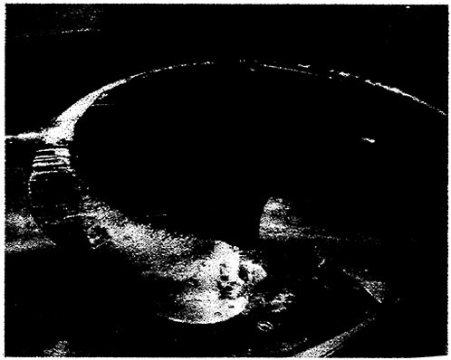
Figure 10: Photograph of the cavitating 4990 hydrofoil inside the DTMB 36inch cavitation tunnel; a=0° σ=0.62. Courtesy of Dr. Edwin Rood of ONR and Dr. Stuart Jessup of DTMB.
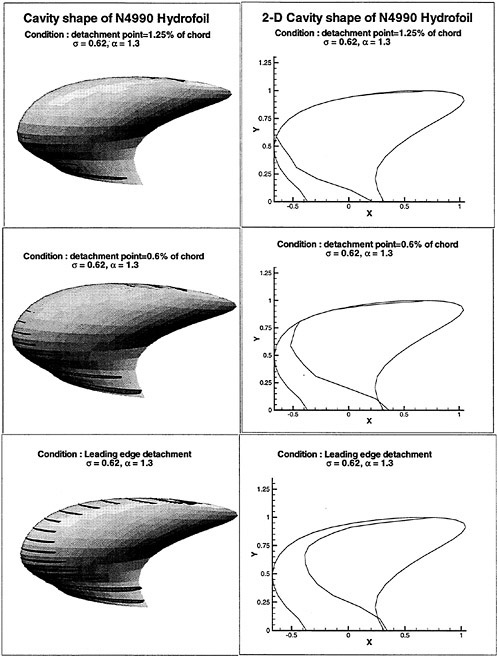
2 Face cavitation
In both the leading edge and mid-chord formulations, cavitation is assumed to occur on the suction side of the propeller blades. For most applications, this is the proper assumption. However, when analyzing propellers at advance ratios which are higher than the design advance ratio, it is found that cavitation may occur on the pressure side (face) of the propeller blades. Thus, face cavitation may occur when the propeller is rotating slowly relative to the inflow velocities. Face cavitation is also common for propellers working in a non-uniform flow field. In these cases, the propeller designed to produce a certain mean thrust may experience smaller loading at the bottom of the revolution. This in turn may create a negative angle of attack at certain radial sections of the propeller blade. As a consequence, the face side will have very low pressures (which leads to face cavitation). Another example of the occurrence of face cavitation is for inclined shaft propellers. The inclined shaft effectively creates a large variation in the angle of attack for each blade section depending on the blade’s position in the rotation. Face cavitation is likely to occur during the upward sweep phase of the blade. A final case with a high potential for face cavitation is a controllable pitch propeller. For certain combinations of pitch and inflow conditions, face cavitation may occur. These examples show that there is clearly a need for the correct modeling of face cavitation in propeller design.
Like back cavitation, face cavitation is not necessarily going to detach at the leading edge. A computational tool for the analysis of face cavitation, MPUF-3A (a lifting surface method [13, 6]), presently can predict leading edge face cavitation. PROPCAV, a panel method [10, 5], was recently modified to predict back cavitation starting at locations on the blade which are determined via an algorithm [15]. In this section the panel method is extended to allow for the prediction of face cavitation with arbitrary cavity detachment.
2.1 Numerical Implementation
The original suction side formulation is used as a foundation for the face side formulation. However, many of the relevant indices need to be changed for the face side formulation. Additionally, all of the involved extrapolations must be correctly indexed. Figure 12 shows a blade section which is exhibiting face cavitation. Solving the problem is similar to solving the back cavitation problem, except that the dynamic boundary condition and kinematic boundary condition must be applied on different regions of the blade. Thus, a need arises to modify the indices
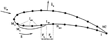
Figure 12: Relevant indices for face cavitation numerical implementation
for the application of Green’s formula:
-
Nwet is the number of panels on the pressure side which are fully wetted. In the case of Figure 12, there are 5.
-
Isp is the panel number of the split panel. In the case of Figure 12, it is the 6th panel.
-
Jcav is the number of cavitating panels, excluding the split panel. In the case of Figure 12, Jcav =3.
-
M0 and M−1 indicate the panels between which the cavity detaches. In the case of Figure 12, they are the 10th and 9th panels, respectively.
-
NC is the number of panels per blade section. In the case of Figure 12, there are 20.
The discretized Green’s formula for partial face cavitation on one blade section based on these indices is shown in equation (17).
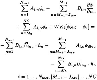
(17)
A, B, and WK are the dipole, source, and wake influence coefficients, respectively. ![]() represents the perturbation potential on the cavity surface. It is determined from the following equation:
represents the perturbation potential on the cavity surface. It is determined from the following equation:
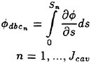
(18)
where Sn is the arclength from the cavity leading edge to the cavity at a position on the blade section n. ![]() on the cavity is determined from the dynamic boundary condition [15]. The i subscripts in equation (17) are equation indices. Each time i is advanced by one, a new equation is being set up. The equation index, i, will be seen again below.
on the cavity is determined from the dynamic boundary condition [15]. The i subscripts in equation (17) are equation indices. Each time i is advanced by one, a new equation is being set up. The equation index, i, will be seen again below.
Even in its present condition, equation (17) does not include the extrapolation terms, namely ![]() at the cavity leading edge, and the source and dipole strength extrapolations for the split panel. Equation (17) is given in its present form for simplicity. However, the following terms need to be added to either the left hand or the right hand sides of equation (17).
at the cavity leading edge, and the source and dipole strength extrapolations for the split panel. Equation (17) is given in its present form for simplicity. However, the following terms need to be added to either the left hand or the right hand sides of equation (17).
-
 extrapolation at the cavity leading edge.
Note that the extrapolation in the case of back cavitation still applies[5, 15]. However, the cavity now is on the pressure side.
 is still the closest to the cavity and
  is still the farthest,
  contributes to equation (17) on both the left and right hand sides. The following terms are added to the left hand side of equation (17):
(19)
where ξi is the sum of the dipole influence coefficients over the cavity surface corresponding to the equation index i:
(20)
The following is added to the right hand side of equation (17):

(21)
where q0 is the known cavity velocity at the detachment point.
-
Source strength extrapolation at the left side of the split panel.
The contribution of the unknown source strength to the left hand side of equation (17) will be the following terms (we call I=Isp for simplicity):
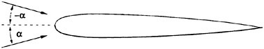
Figure 13: Symmetric hydrofoil for validation of face cavitation. NACA66 thickness distribution, t/c=0.05. Span/c=2.0.
-
FL is the fraction of the split panel which is beneath the cavity and FR is the fraction of the split panel which is wetted. QTA is the source strength extrapolation coefficient. In cases where the cavity is not at least four panels in length, the extrapolation is simplified by eliminating terms beginning with the QTD term. This is easily accomplished in the code by setting QTD equal to zero. On the right hand side, the following terms contribute to equation (17):
(22)
-
Dipole strength extrapolation at the right side of the split panel.
A similar extrapolation takes place on the wetted half of the split panel. The unknown terms that will contribute the the left hand side of equation (17) are as follows:
(23)
Again, terms will be dropped if there are not enough panels available for the complete extrapolation [15]. The right hand side contribution will be:
(24)
Equation 17 now sets up the system of equations to be solved using a block iterative matrix solver [4].
2.2 Validation
The face cavitation modifications to the code are validated against the code’s original back cavitation formulation. This is done by using a symmetric rectangular hydrofoil that is subjected to flow at an angle of attack of ±α as shown in Figure 13. Under
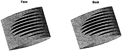
Figure 14: Cavity planforms for face and back cavitation on a rectangular hydrofoil. 50×10 panels. σ=0.3. α=±3°. Leading edge detachment. Cosine panel spacing chordwise. Constant panel spacing spanwise.
such conditions, a hydrofoil will show cavitation on the face side which is equivalent to cavitation on the back for the opposite angle of attack. The option to run PROPCAV in “hydrofoil mode” is a modification that is described in more detail in [15].
Figure 14 shows the cavity planforms predicted on the symmetric hydrofoil for the face and back cavitation comparisons. The detachment location is the leading edge, so the cavity detaches at the same location on the foil for both face and back cavities. The planforms agree well.
The method is further validated by comparing the results for a non-leading edge detachment case. This time, the detachment was at the third panel at all spanwise strips. This equates to a detachment at 3.5% of the chordlength aft of the leading edge. The cavity planform is shown in Figure 15. Notice that both Figures 14 and 15 have the same cavitation number. However, the cavities are dramatically different. This emphasizes the importance of choosing the correct detachment point. For these cases, the actual detachment would be at or very close to the leading edge. For the given conditions, Figure 14 corresponds to the more realistic prediction.
As with the mid-chord back cavitation problem, there are conceivably cases where the cavity would not detach at the leading edge in the case of face cavitation. We are therefore interested in examining a case where mid-chord face cavitation is likely. A hydrofoil with camber is used for this study (Figure 16). For the face cavitation case, the camber is −0.02 f/C. For back cavitation is is +0.02 f/C. The angle of attack was also decreased to ±1.0°. Thus, the problem is still symmetric and should have the same solution (on opposite sides) for both face and back cavitation.
Figure 17 shows the wetted pressure on the cavitating side of the rectangular hydrofoil with camber.
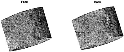
Figure 15: Cavity planforms for face and back cavitation on a rectangular hydrofoil. 50×10 panels, σ=0.3. α=±3°. Detachment at 3.5% x/c. Cosine panel spacing chordwise. Constant panel spacing spanwise.
Figure 16: Hydrofoil with camber. Camber/C=±2%. Meanline=0.8 camber distribution. t/C=5%. NACA66 thickness distribution. ±α=±1.0°
A value of σ=0.23 is chosen so that mid-chord cavitation is likely. Figure 18 shows the cavity planforms for these two cases, each predicted in an independent run. Figure 19 shows the cavity volume convergence history for the two runs. Note that the abscissa is in propeller revolutions. Although the hydrofoil case was a steady flow run, the computations still progressed in a propeller-like fashion i.e the fully wetted flow is first solved followed by the cavitating flow.
Figure 19 seems to indicate an un-converged value of volume near the final revolutions. It would appear from this figure that the cavity planform has not converged. However, the cavity thicknesses in this case are extremely thin. Since the cavities predicted for mid-chord cavitation are so thin, it is dif-
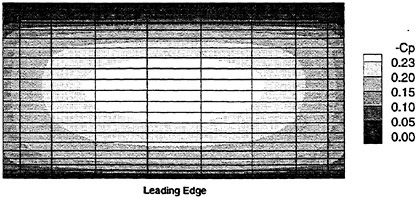
Figure 17: Wetted pressure distribution on hydrofoil with camber. 50×10 panels, α=±1.0°. Camber/c =±0.02. t/c=0.05.

Figure 18: Cavity shapes for mid-chord face and back cavitation on the rectangular hydrofoil. 50×10 panels, α=±1.0°. Camber/c=±0.02. t/c=0.05. σ=0.23.
ficult to obtain a completely smooth volume plot. Even in reality, mid-chord cavities on a hydrofoil are known to be very unstable. With very thin cavities, there may be a relatively large variation in cavity length even when the cavity has closed to within the specified tolerance. This variation may contribute to slight unsteady effects which are inherent in the propeller code, such as the unsteady effect of the wake. These slight instabilities may be the cause of the jagged volume plot. In any case, the figure shows that the volume for the face and back predictions converges to the same range of values. Further confidence in the face cavitation model is supported by Figure 20, which shows that the predicted final detachment locations for the face and back cases match each other exactly. This can also be seen in Figure 18.
2.3 Convergence
The convergence of the mid-chord face cavities on the hydrofoil was studied. Several panel discretizations were used in this study, ranging from 50×10 to 100×20. There are three important convergence issues that were considered:
-
Detachment Location Convergence
-
Cavity Shape Convergence
-
Cavity Volume Convergence
Figure 21 shows the final detachment lines for several panel configurations. The abscissa is the spanwise position and the ordinate is the chordwise detachment location. Only the strips which were cavitating are shown. The detachment lines are very close to each other for all panel discretizations with the maximum variation being about 3% near the outermost cavitating strips. The resulting cavity shapes for
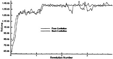
Figure 19: Cavity volume for mid-chord face and back cavitation on a rectangular hydrofoil. 60×12 panels, α=±1.0°. Camber/c=±0.02. t/c=0.05. σ=0.23.
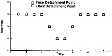
Figure 20: Final detachment locations for mid-chord face and back cavitation on a rectangular hydrofoil. Ordinate is panel number from leading edge. Abscissa is strip number. 60×12 panels, α=±1.0°. Camber/c=±0.02. t/c=0.05. σ=0.23.
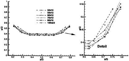
Figure 21: Final detachment lines for 6 runs, α=−1.0°. Camber/c=−0.02. t/c=0.05. σ=0.23. Grids: 50×10, 50×12, 60×12, 70×12, 80×12, 100×20.
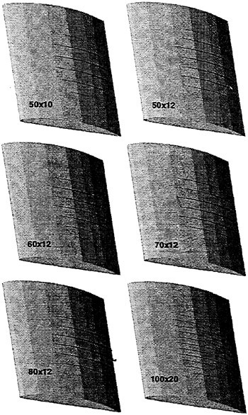
Figure 22: Cavity shapes for 6 runs, α=−1.0°. Camber/c=−0.02. t/c=0.05. σ=0.23. Panels =50×10, 50×12, 60×12, 70×12, 80×12, 100×20. Cosine panel spacing chordwise. Constant panel spacing spanwise.
these runs may be seen in Figure 22. The figure indicates that there are differences in cavity heights for certain panel discretizations. However, the general cavity shapes are consistent with each other. Nevertheless, these noticeable differences in cavity lengths and heights have caused a non-converging cavity volume. It is possible that even 100×20 panels are not enough for convergence.
2.4 Results
The face cavitation formulation is now applied to a propeller. The advance ratio is much higher than the design advance ratio (which is 1.2). Such a high advance ratio will incite face cavitation. The propeller used is a modified version of the N4990 propeller (called N4990-IP), which is designed to limit cavitation near the tip by having an increased pitch near the tip. The geometry is given in Appendix A. The run is performed under steady conditions. The
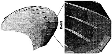
Figure 23: Cavity planform for face cavitation as predicted by PROPCAV. 50×10 panels. Js=2.0. σn=5.5.
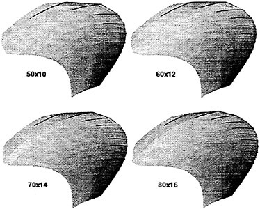
Figure 24: Cavity planform for face cavitation as predicted by PROPCAV. 50×10, 60×12, 70×14, 80×16. Js=2.0. σn=5.5.
inflow wake is uniform and the Froude number is very large. In addition: Js=2.00, σn=5.50, grid: 50×10
The cavity planform for the run is shown in Figure 23. The plot is three dimensional, but this cannot be seen except close to the blade. A detail of the cavity at strips 3, 4, and 5 is shown in Figure 23.
2.5 Convergence
The cavity planforms for 50×10, 60×12, 70×14, and 80×16 panels are shown in Figure 24. These planforms indicate that the general shape of the cavity is not changing for an increasing number of panels. Near the hub, slightly more cavitation can be seen for the 80×16 case. This may be due to a better resolution of the blade near the hub. In general, propeller blades are thicker near the hub. In order to completely resolve the rapid change in thickness near the hub, more panels may be required.
2.6 Comparison to MPUF-3A
The results of this run are compared to a face cavitation prediction from MPUF-3A [6]. The conditions are the same. The resulting cavity planform is shown in Figure 25. A direct visual comparison of the cavity thicknesses cannot be made in this case because the cavities are plotted normal to a 3-D blade in PROPCAV, while MPUF-3A overlays 2-D thickness plots onto a blade profile.
3 Developed tip vortex cavity
A developed tip vortex is shown in Figure 26. The blade geometry at the tip has been modified in order to prevent the presence of a blade cavity connected to the tip vortex cavity, since the objective of this stage is to model the tip vortex cavity shape away from the blade.
The governing equation in the case of potential flow (a reasonable assumption in the case of a developed tip vortex cavity) is Green’s 3rd identity as described in previous sections. A dynamic boundary condition of constant vapor pressure is applied on the tip cavity while a kinematic boundary condition is applied on the wetted part of the blade. This is depicted in Figure 26. The surface of the tip vortex cavity will be determined from applying the kinematic boundary condition on the cavity surface. In the present work we have completed the development of a method for determining the cavity shape away from the trailing edge. The following special case will be used in order to demonstrate the validity of the method. This is the case of a vortex horseshoe in the vicinity of a bulb as shown in Figure 27. The vortex horseshoe has a strength equal to Γ while the whole system is subject to a uniform flow at an angle of attack α. In order to facilitate the analysis we relate the angle of attack and vortex strength so that the vortex trajectory is parallel to the x axis far downstream (i.e. the down-wash is equal to the vertical component of the inflow velocity):
(25)
If Φ is the total velocity potential, then the pressure coefficient2CP will be given from:
(26)
where υ and s are the orthogonal curvilinear coordinates on the surface of the tip vortex cavity, with υ being along the circumference.
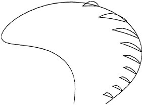
Figure 25: Cavity planform for face cavitation as predicted by MPUF-3A. 20×9 panels. Js=2.0. σn=5.5.
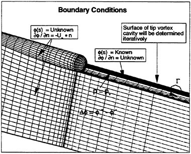
Figure 26: The boundary conditions in the vicinity of a developed tip vortex. For simplicity, in this figure an isolated tip vortex cavity is considered at the end of a “bulbous” tip, especially designed in order to avoid mixed tip/blade cavity.
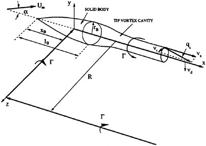
Figure 27: Developed tip vortex cavity in the bulb and the horseshoe problem.
On the cavity −CP=σ. Equation (26) then becomes the dynamic boundary condition on the tip vortex cavity:
(27)
Far downstream the shape of the cavity will not vary with s. In addition, the horizontal velocity will have to be equal to U∞ cos α. Equation (28) thus becomes:
(28)
The above equation requires that the circumferential velocity is constant around the vortex.
The shape of the tip vortex cavity will not be circular (even far downstream), and the objective of this work is to determine this cavity shape. To do this, first we assume that the tip vortex is circular. This results into a tip vortex radius, ro, given from the expression:
(29)
We then apply a boundary element method on the tip vortex cavity (assuming that it is a solid body) and determine a pressure distribution around the tip vortex which is expected to vary along the circumference. We next determine the potentials on the tip vortex cavity by integrating the value of ∂Φ/∂s along s, as given by equation (27), where ∂Φ/∂υ is taken from equation (28) in the first iteration and from the previous iteration in subsequent iterations. With the known potentials on the tip vortex cavity we determine the value of ![]() using the BEM and Green’s identity. The radial location around the tip vortex is then adjusted at each section by using the equation:
using the BEM and Green’s identity. The radial location around the tip vortex is then adjusted at each section by using the equation:
(30)
where h is the adjustment of the tip vortex radius along υ. The new shape is adjusted so that the total circumference is the same as before (since the strength of the tip vortex has to be the same). This procedure is repeated several times until the cavity shape does not change within a certain tolerance. Figure 28 shows the predicted converged tip cavity sectional shape far downstream in the case α=4° and σ=0.4866. Figures 29 and 30 show the corresponding pressure distribution from the first and the last iterations. Note that −CP is varying around the tip circumference in the first iteration (when the tip vortex cavity is taken to be a circular cylinder) but is constant and equal to the cavitation number
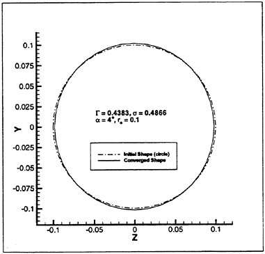
Figure 28: Tip vortex cross-section from the first and last iteration.
in the last iteration. Figure 31 shows the predicted converged tip cavity sectional shape far downstream with varying number of circumferential panels in the case of α=4° and σ=0.1. Note that the cavity shape converges quickly with number of circumferential panels. Figures 28 and 31 correspond to two cases with the same α (thus the same vortex strength Γ) but different cavitation numbers. In the case of smaller cavitation number, shown in Figure 31, the cavity sectional area is larger (as expected) but also the converged cavity shape is farther from the initial circle.
4 Conclusions
A panel method for the prediction of the unsteady sheet cavitation on hydrofoils or propeller blades was extended to include:
-
effects of tunnel walls. The effects were found to be critical in predicting the correct cavity shape observed in experiments.
-
face cavitation with arbitrary detachment. The method was applied to 3-D hydrofoil and propeller geometries.
-
developed tip vortex cavity. The method predicted a non-circular tip vortex cavity shape by requiring a constant pressure distribution on it.
The convergence of the method was studied extensively. Matching the tip vortex with the blade cavity and comparisons with experiments are some of the topics that need to be addressed in the near future.
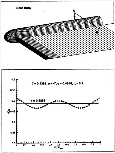
Figure 29: −CP vs. υ/υmax at section A—A of the “solid body” tip vortex. The panels representing the bulb and the tip vortex cavity are shown at the top.
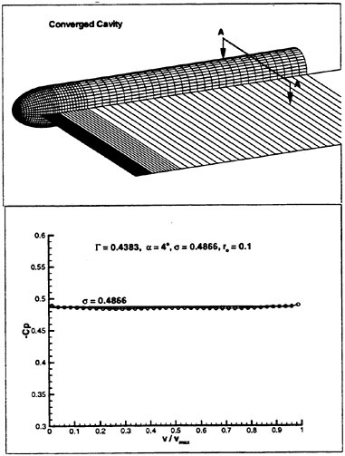
Figure 30: −CP vs. υ/υmax at section A—A of the tip vortex cavity. The panels representing the bulb and the tip vortex cavity are shown at the top.
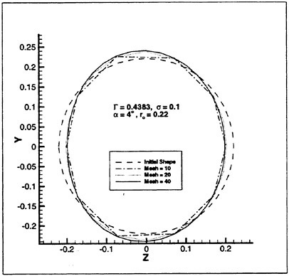
Figure 31: Convergence of the tip vortex cross-section with number of panels along the circumference.
Acknowledgment
Support for this research was provided by the following companies and research centers: Daewoo Heavy Industries Ltd., David Taylor Model Basin, El Pardo Model Basin, Hamburgische Schiffbau-Versuchsanstalt, Hyundai Heavy Industries Co. Ltd., KaMeWa AB, Michigan Wheel Corporation, Rolla SP Propellers SA, Sulzer-Hydro GmbH, Ulstein Propeller AS, Volvo-Penta of the Americas, and Wärtsilä Propulsion. The authors wish to thank Dr. Edwin Rood of the Office of Naval Research and Dr. Stuart Jessup and Dr. Scott Black of David Taylor Model Basin for providing them with the data for the 4990 hydrofoil experiment.
References
[1] W.H.Brewer and S.A.Kinnas. Experiment and viscous flow analysis on a partially cavitating hydrofoil. Journal of Ship Research, 41(3):pp. 161–171, September 1997.
[2] J.-K.Choi and S.A.Kinnas. Cavitating propeller analysis inside of a tunnel. In Cavitation and Multiphase Flow Forum, Vancouver, Canada, June 1997. Fluids Engineering Division, ASME.
[3] J.-K.Choi and S.A.Kinnas. Numerical water tunnel in two and three dimensions. Journal of Ship Research, 42(2):pp. 86–98, June 1998.
[4] R.W.Clark. A new iterative matrix solution procedure for three-dimensional panel methods. In 23rd Aerospace Sciences Meeting, Reno, Nevada, January 1985. AIAA.
[5] N.E.Fine. Nonlinear Analysis of Cavitating Propellers in Nonuniform Flow. PhD thesis, Department of Ocean Engineering, MIT, October, 1992.
[6] P.E.Griffin. Computational techniques for the design and analysis of cavitating propeller blades. Master’s thesis, UT Austin, Dept. of Civil Engineering, May 1998.
[7] S.Jessup, 1997. private communication.
[8] S.Jessup, W.Berberich, and K.Remmers. Cavitation performance evaluation of naval surface ship propellers with standard and advanced blade sections. In Twentieth Symposium on Naval Hydrodynamics, pages 101–116, University of California, Santa Barbara, August 1994.
[9] S.A.Kinnas. Prediction of unsteady sheet cavitation. In Third International Symposium on Cavitation, pages 19–36, Grenoble, France, April 7–10 1998.
[10] S.A.Kinnas and N.E.Fine. A nonlinear boundary element method for the analysis of unsteady propeller sheet cavitation. In Nineteenth Symposium on Naval Hydrodynamics, pages 717–737, Seoul, Korea, August 1992.
[11] S.A.Kinnas and N.E.Fine. A numerical nonlinear analysis of the flow around two- and three-dimensional partially cavitating hydrofoils. Journal of Fluid Mechanics, 254:151–181, September 1993.
[12] S.A.Kinnas, S.Mishima, and W.H.Brewer. Nonlinear analysis of viscous flow around cavitating hydrofoils. In Twentieth Symposium on Naval Hydrodynamics, pages 446–465, University of California, Santa Barbara, August 1994.
[13] C.-S.Lee. Prediction of Steady and Unsteady Performance of Marine Propellers with or without Cavitation by Numerical Lifting Surface Theory. PhD thesis, M.I.T., Department of Ocean Engineering, May 1979.
[14] S.Mishima, S.A.Kinnas, and D.Egnor. The CAvitating PRopeller Experiment (CAPREX), Phases I & II. Technical report, Department of Ocean Engineering, MIT, August 1995.
[15] A.C.Mueller. Development of face and mid-chord cavitation models for the prediction of unsteady cavitation on a propeller. Master’s thesis, UT Austin, Dept. of Civil Engineering, May 1998.
[16] A.C.Mueller and S.A.Kinnas. Cavitation predictions using a panel method. In ASME Symposium on Marine Hydrodynamics and Ocean Engineering, volume 14, pages 127–137, Dallas, TX, November 16–21 1997.
A Blade geometries
Table 1: The geometric characteristics of the 4990 hydrofoil; extracted from the data of Jessup (1997); xm and zm are the coordinates of the mid-chord line; twist is defined as the angle between the nose-tail line and the x axis.
|
r/R |
Twist (degs) |
xm/D |
zm/D |
c/D |
f/C |
t/D |
|
0.000 |
−8.00 |
−0.0135 |
0.002 |
0.3442 |
−0.030 |
0.0707 |
|
0.100 |
−1.06 |
−0.0429 |
0.006 |
0.3482 |
−0.011 |
0.0513 |
|
0.200 |
3.88 |
−0.0757 |
0.011 |
0.3894 |
−0.005 |
0.0424 |
|
0.300 |
8.04 |
−0.0904 |
0.014 |
0.4394 |
0.019 |
0.0414 |
|
0.400 |
10.72 |
−0.0846 |
0.014 |
0.4996 |
0.028 |
0.0410 |
|
0.500 |
10.63 |
−0.0599 |
0.011 |
0.5596 |
0.030 |
0.0408 |
|
0.600 |
8.67 |
−0.0182 |
−0.004 |
0.6157 |
0.028 |
0.0392 |
|
0.700 |
6.20 |
0.0400 |
−0.009 |
0.6645 |
0.024 |
0.0366 |
|
0.800 |
3.24 |
0.1155 |
−0.024 |
0.6853 |
0.019 |
0.0331 |
|
0.900 |
0.10 |
0.2098 |
−0.037 |
0.6154 |
0.014 |
0.0265 |
|
0.950 |
−1.52 |
0.2667 |
−0.042 |
0.4920 |
0.012 |
0.0205 |
|
0.975 |
−2.38 |
0.2974 |
−0.043 |
0.3730 |
0.011 |
0.0155 |
|
1.000 |
−3.25 |
0.3289 |
−0.045 |
0.1000 |
0.000 |
0.0000 |
Table 2: The geometry of DTMB N4990-IP (Increased Pitch at Tip). 5 blades. NACA66 thickness distribution. a=0.8 meanline camber distribution
|
r/R |
P/D |
Rake |
Skew |
C/D |
f/C |
t/D |
|
0.30 |
1.183 |
−0.0004 |
0.00 |
0.1776 |
0.00202 |
0.04442 |
|
0.35 |
1.360 |
−0.0123 |
−4.53 |
0.2099 |
0.00533 |
0.03820 |
|
0.40 |
1.516 |
−0.0237 |
−7.53 |
0.2412 |
0.01059 |
0.03377 |
|
0.45 |
1.642 |
−0.0338 |
−9.21 |
0.2714 |
0.01657 |
0.03121 |
|
0.50 |
1.731 |
−0.0414 |
−9.75 |
0.3020 |
0.02297 |
0.03041 |
|
0.60 |
1.795 |
−0.0458 |
−7.96 |
0.3620 |
0.02980 |
0.02929 |
|
0.70 |
1.719 |
−0.0395 |
−3.12 |
0.4200 |
0.02834 |
0.02780 |
|
0.80 |
1.547 |
−0.0278 |
4.12 |
0.4690 |
0.02036 |
0.02533 |
|
0.90 |
1.500 |
−0.0141 |
13.41 |
0.4650 |
0.00932 |
0.02102 |
|
0.95 |
1.500 |
−0.0072 |
18.82 |
0.3900 |
0.00333 |
0.01642 |
|
1.00 |
1.400 |
0.0000 |
24.74 |
0.0010 |
−.00270 |
0.00000 |
The Application of ‘RANS’ Code to Investigate Propeller Scale Effects
M.Stanier (Defence Evaluation and Research Agency, United Kingdom)
Abstract
This paper describes the application of a Reynolds Average Navier-Stokes Solver code for marine propellers to investigate propeller scale effects. A 3 blade model propeller was evaluated with two different mesh regimes which have been used to improve blade wake flow feature capture. The propulsion predictions from the RANS code agreed well with the model test propulsion experiments. Propeller blade to blade and wake predictions have been investigated. The predicted velocities have been compared with laser doppler velocity measurements and show close agreement. Propeller scale effect has been investigated for both a 3 blade propeller and two 5 blade propellers. The investigation evaluated the scale effect on propulsion and the flow field. The flow field results showed a significant scale effect on vortex flow resulting in changes to the propulsive performance between the model and full size propellers.
1 Introduction
DERA Haslar has developed an advanced propeller analysis capability with the use of a Reynolds Averaged Navier-Stokes (RANS) code. This capability also includes the mesh generator (pre-processing) and inspection tools (post-processing), and has been applied to a series of model size straight 5 blade propellers, Stanier (1992, 1994).
This paper describes the application of a RANS code to investigate the effect of propeller size on the performance of marine propellers. The first section of the paper briefly describes the code, whilst the second section describes the application, at model scale, of the code to a 3 blade propeller. The third section describes the effect of propeller size on the three blade propeller used in section two. The fourth section describes the effect of propeller scale effect on two modern skewed 5 blade propellers.
The three bladed propeller (Denny 1968) was chosen since a comprehensive set of laser measurements are available (Jessup 1989 and 1994). Following the evaluation stage the objectives were to verify the propulsive performance predictions at design and off-design conditions at model scale and to compare the difference between the predictions at a typical full scale size and the model size. The flow field around the propeller blades at the two different sizes were compared which allowed the effects of scale to be investigated.
Two modern skewed 5 blade propellers were then investigated to see whether or not these propellers exhibited any significant scale effects.
The numerical prediction at model scale used a propeller diameter of 0.3048 m which corresponded to the propeller diameter used in the experimental tests. This gave a blade section Reynold’s Number of 0.6×10⁶ for the three blade propeller. The numerical predictions at full scale used a scale factor of 20 and gave a propeller diameter of 6.096 m with a corresponding Re of 32.2×10⁶.
One of the most important areas of RANS code work is the development of the propeller analysis mesh on which the calculations are to be carried out. For the 3 blade propeller two different meshing regimes were used. The first was used for the propulsion predictions whilst the second was used for the investigation of the detailed flow allowing better definition of the tip and blade wake predictions. For the 5 blade propeller only
©British Crown copyright 1998. Reproduced with the permission of the Controller of Her Majesty’s Stationery Office. The views expressed are those of the author and do not necessarily reflect the views or policy of The Ministry of Defence, Her Majesty’s Stationery Office, or any other British government department.
one mesh regime was used.
2 Description of the RANS code
The equations governing fluid flow around a propeller blade are the Navier-Stokes equations. The continuity equation simply states that the rate of change of mass within the control volume equals the rate of mass flux. The momentum equation states that the rate of change of momentum within the control volume is equal to the rate at which momentum is entering and leaving through its surfaces, plus the sum of the forces acting on the volume due to the normal and tangential forces (including pressure and shear stress forces). The energy equation for the fluid states that the rate of change of internal energy within the control volume is equal to the rate at which enthalpy is entering, plus work done on the volume by the viscous stresses on the boundary. These five equations (1 continuity, 3 momentum, 1 energy) are all that is needed to evaluate the compressible flow through a blade passage. The present RANS code uses a three dimensional finite volume approach to solve for the incompressible flow using the continuity and momentum equations.
The flow variables are stored at the centre of each cell and the fluxes through the cell faces are found by linear interpolation of these values. Since all the volumes share common faces, except at the inflow, outflow and solid boundaries, global conservation of the flow properties is automatically obtained. The conditions of zero flux of mass and momentum are imposed through the cell faces in contact with a solid boundary.
The pressure field is obtained using the method of artificial compressibility. At low Mach numbers, compressible time-marching flow solvers perform poorly due to unfavourable interactions between long-wavelength errors and the inflow and outflow boundaries. The decay of the long-wavelength errors becomes increasingly retarded and convergence is slowed or even prevented at low Mach numbers. Long-term convergence rate are dominated by long-wavelength errors, which travel up and down the flow domain interacting with the inflow and outflow boundaries. The artificial compressibility method replaces the density term in the equation of mass continuity by a pressure term via an artificial acoustic speed term β. This allows the incompressible flow to be computed and is valid for converged steady state flows.
A multigrid acceleration technique is used to increase the rate of convergence. The basic philosophy of this approach is to allow information regarding the overall flow pattern to propagate rapidly on a coarse grid. This method consists of combining groups of cells into a single block. Each block can then be thought of as a larger single cell, such that the flux values on each face are equal to the sum of the flux values from the original smaller cells. Each block is then treated in the same way as a smaller cell using the same solver software.
The major influence of viscous effects on the flow patterns in the blade rows of most turbomachines is known to be the effective reduction in passage area caused by the boundary layer growth. Any turbulence model that simulates correctly the blockage in the blade passage is likely to give good results. A mixing length model (3D version of Baldwin-Lomax) is used to represent the effects of turbulence in this code. The basis of any turbulence model is to infer the appropriate length and velocity scales and in the case of a mixing length method both of these scales are obtained from the mean flow. This method uses global flow parameters giving good overall predictions of total losses.
3 Validation using a 3 Blade Propeller
Model propeller DTRC4119 was chosen as part of the validation exercise of the code since extensive laser velocity measurements have been made around this propeller (Jessup 1989) and uncertainty analysis has been carried to confirm the validity of the measurements (Jessup 1994).
3.1 Propeller Geometry and Meshing
Model propeller (DTRC4119) has three straight blades with a conventional blade section consisting of a TMB-modified NACA-66 thickness form and a NACA a=0.8 camber line. The detailed propeller geometry can be found in Denny (1968).
The RANS code required the blade passage to be discretised into a series of hexahedral cells. These were defined by the intersections of three curved planes; the first set of planes are cylindrical with the first plane lying on the propeller hub and subsequent planes having larger radii, the second set of planes radiate from the shaft centre line, whilst the third set of planes are at
right angles to the shaft centre line, see Figure 1.
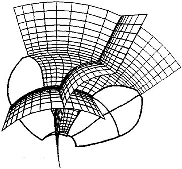
Figure 1 Propeller Mesh Construction
The blade to blade mesh needs to be aligned with the blade surface and with the axial direction, both upstream and downstream of the propeller to prevent significant distortion of the mesh. This distortion can result in slow, or no, convergence of the solver. There is a region just upstream and downstream of the propeller where the mesh can also be aligned with the local flow. For propulsion predictions the blade to blade mesh is shown in Figure 2 and was used as it gave good convergence. For the flow predictions the mesh shown in Figure 3 was used as this mesh had been aligned with the blade wake.
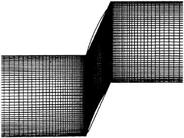
Figure 2 Non-Aligned Mesh
The propeller hub and upstream fairing cone were modelled as an infinitely long constant radius cylinder. This was required to prevent the mesh becoming degenerative on the shaft centre line. The tip was modelled with a finite chord length and zero thickness, again to prevent the mesh becoming degenerate.
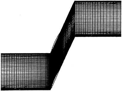
Figure 3 Wake Aligned Mesh
The mesh used in these calculations had 458297 nodes formed by 199 node planes from inlet to exit, 49 planes from blade surface to blade surface and 47 planes from the hub to the outer radial limit. The inlet was set at four propeller diameters upstream of the propeller mid-plane, whilst the exit was set at four propeller diameters downstream. The outer radial limit was set at 3.5 times the propeller diameter.
3.2 Propulsion Predictions
The predicted propulsive performance curves, along with the open water experimental results from Denny (1968) and Jessup (1989) are shown in Figure 4.
The predicted thrust and torque at the design advance coefficient show close agreement with the model test results, the difference in thrust and torques are 0.7% and 2.5% respectively. The accuracy of the RANS code predicted thrust slowly deteriorates with reduced advance coefficient. As with the model experiments in the Cavitation Tunnel the choice of axial velocity for use in the definition of J is not clear cut for the predictive results. The value used was the average axial velocity component over the annular disk
occupying approximately half the area between the propeller tip and the outer radial limit at the propeller axial mid line (directrix). A different definition could result in a different value of advance coefficient, J.
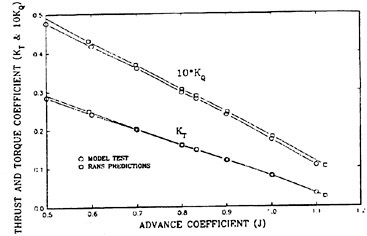
Figure 4 Propulsion Predictions
3.3 Flow Predictions
The effect of the downstream mesh on the wake predictions can be seen in Figure 5 for the predictions of axial velocity for the two meshs given in Figures 2 and 3. At axial locations x/R=0.25 and x/R=0.304 the predicted axial velocities show similar agreement. For axial locations beyond x/R=0.304 and up to x/R=0.808 the plots for the wake aligned mesh (Figure 3) show that the wake structure has been captured whilst for the non-aligned mesh (Figure 2) the wake structure does not appear in the predictions. For axial location greater than x/R=0.808 neither of the mesh schemes appears to capture the wake.
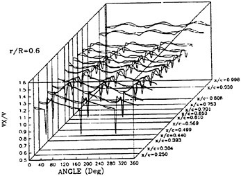
Figure 5 Variation of Axial Velocity with Mesh
The choice of meshing scheme has a significant effect on wake feature capture and care is required to choose the appropriate meshing scheme.
3.4 Mean Inflow Velocities
The mean axial and radial inflow velocities at X/R=−0.3 for numerical and model test cases are given in Figure 6 and there is a difference for the inner blade span. The most likely explanation for this difference is the infinitely long constant radius hub used in the predictions as compared with the real hub and nose fairing. The experimental flow will have been perturbed away from the uniform inflow condition by the hub fairing cone. In the case of the numerical predictions this radial perturbation will not be present, but the effect of a larger boundary layer due to the long cylindrical hub can be seen in the axial velocity predictions. These differences are generally small but can still have an effect on the convected portion of the flow.
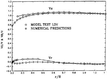
Figure 6 Mean Inflow Velocities
3.5 Mean Wake Predictions
The mean axial, radial and tangential velocities at X/R=0.329 are given in Figure 7. The axial velocity shows close agreement between the measured and predicted values. There is a small difference between the measured and predicted values near the propeller tip radius, reflecting a different location for the tip vortex. The small difference in mean axial velocity is also reflected in the good thrust prediction agreement between the model and predicted values of KT.
The mean radial velocity at X/R=0.329 shows
that the model test results have a larger inward radial velocity compared to the predicted values. There are several reasons for this difference; one being the effect of the location of the outer radial boundary and the other being a failure in the solver/meshing. The results of this difference in predicted and measured radial velocities will be the radial location of the individual flow features such as the tip vortex, with the model test results having a smaller contraction radius.
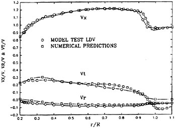
Figure 7 Mean Wake Velocities X/C=0.329
The tangential velocity at X/R=0.329 shows generally close agreement between the predicted and measured values, except in the tip region. Again the agreement is reflected in the good torque predictions for the propeller, which agree well with the measured values but are not as close as those for the thrust predictions.
3.6 Detailed Blade to Blade Predictions
The blade to blade Vx, Vr and Vt predictions at X/R=0.0, for a radius of r/R=0.7 are given in Figure 8 to 10, respectively. The axial velocities (Figure 8) generally show good agreement with the measured velocities values. Near the blade surface the are slight differences between the predictions and the measured values. This may be due to inadequate meshing or turbulence modelling.
The radial velocities (Figure 9) do not show as good an agreement as the axial velocity values. Although the magnitude of the difference is a small fraction of the axial velocity. The shape of the predictions agrees well with the experimental results.
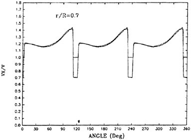
Figure 8 Blade to Blade Axial Velocities
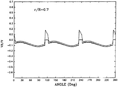
Figure 9 Blade to Blade Radial Velocities
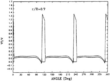
Figure 10 Blade to Blade Tangential Velocities
The shape of the tangential velocity (Figure 10) again shows close agreement with that measured, with a difference in the mean value. Again there is a difference near the blade surface.
3.7 Detailed Wake Predictions
The detailed predicted and measured axial radial and tangential velocities in the wake at X/R=0.329, for r/R=0.7 and r/R=0.949, are given in Figures 11 to 13. The predicted tip vortex location at X/R=0.329 was r/R=0.949 which differs from the measured location of r/R=0.924. For completeness the measured velocities at r/R=0.924 are compared with the predictions at r/R=0.949.
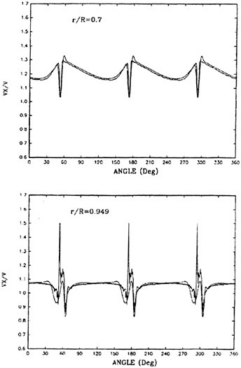
Figure 11 Axial Wake Velocities
Generally, the axial velocity predictions (Figure 11) show close agreement with the model test measurements. The accurate prediction of the minimum value in the wake trough is dependent on the location of the nodes making up the analysis mesh used being directly located at the wake minimum location. This is somewhat unlikely. At a radius of r/R=0.7, the depth and width of the axial velocity wake shows close agreement between the predicted and measured values. The predicted values show a local peak in the axial velocity on the suction side of the blade wake that is not seen in the measured data. This peak may be the result of either poor local mesh placement or the turbulence model used. The predictions at r/R=0.949 are generally in close agreement with the measured values at r/R=0.924, indicating that the measured and predicted tip vortex flows have coincided. Localised differences exist in and near the vortex core and this may be due to the difference in the predicted and measured location of the vortex or due to insufficient mesh resolution in this area.
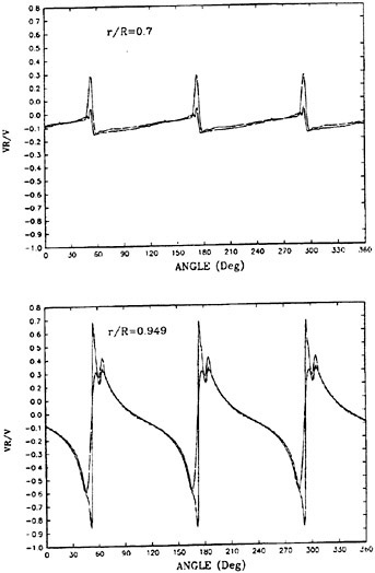
Figure 12 Radial Wake Velocities
The agreement for the radial wake velocity (Figure 12) components is not generally as close as that for the axial velocities above. This was also seen in the mean radial velocity distributions. The predicted maximum in the wake is too high and the wake width is too large. In the vortex flow region the predictions at
r/R=0.949 agree well, with a reasonable match of the double hump in the positive radial velocity values.
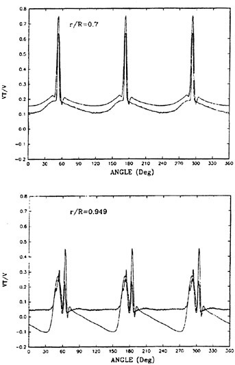
Figure 13 Tangential wake Velocities
The predicted tangential wake velocities (Figure 13) are not as close to the measured values as were the predicted axial wake velocities. This was also the case for the mean tangential velocities and is also reflected in the torque coefficient predictions. The predicted width of the wake is close to the measured values whilst the peak values show some differences. The tangential velocities on the suction side of the wake also show a local minimum that is not present in the model test measurements. This could be due to difficulties with local mesh resolution or turbulence modelling. At the tip vortex radius there are significant differences between the predicted and measured tangential wake velocities. This is most like due to the difference in the actual location of the tip vortex and the numerical position of the tip vortex, the mean tangential values (Figure 7) show significant difference for small changes in the radial location in this region.
4 Scale Effect on a 3 Blade Propeller
Flow predictions have been carried out using the wake aligned mesh, shown in Figure 3. The predictions were carried out at one off-design advance coefficient since the propulsion predictions showed the largest scale effect to occur at the lower advance coefficients. Therefore the flow prediction comparison has only been carried out at an advance coefficient of J=0.5.
4.1 Propulsion Predictions
The predicted propulsive performance curves for model and full scale are shown in Figure 14. The full scale predicted thrust and torque generally have higher values than those predictions made at model scale. At the design advance coefficient the difference in thrust of the full scale propeller was 2% higher than that for the model scale propeller. The torque coefficient for the full scale propeller was 0.3% higher than the predicted values for the model scale propeller.
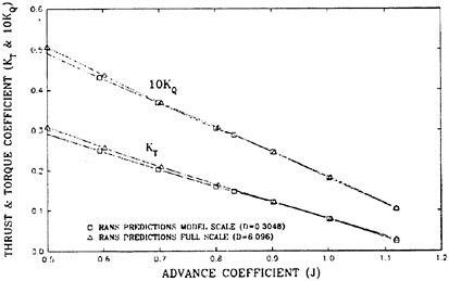
Figure 14 Propulsion Predictions for DTRC4119
Clearly the scale effect can be seen, from Figure 14, to be more significant at the off-design conditions, particularly at reduced advance coefficient, compared to the design advance coefficient.
4.2 Static Pressure Predictions
The blade surface static pressure predictions for the suction side of the propeller blade for the two different scaled propellers are given in Figure 15. The colour contours are of −Cp and the higher the value of
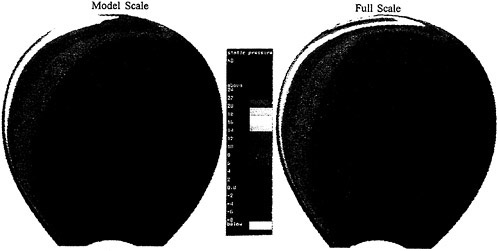
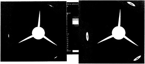
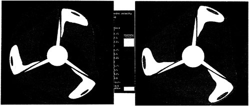
−Cp the lower the static pressure. The principal difference in static pressure distributions on the suction side of the blade occur near the leading edge and tip regions of the blade. This region is associated with the leading edge and tip vortex. The remaining area of the suction side are very similar for the two propellers. This leads to the conclusion that the difference in propulsion is associated with the difference in pressure on the suction blade surface associated with vortex flow structure scale effects.
A transverse section through the propeller at the axial location X/D=0.1 permit the downstream features of the tip region flow to be shown, Figure 16. At this location the two different scale propellers show significant difference in the static pressure in the tip vortex region. The full scale propeller has much larger values of −Cp and is associated with a much larger and more powerful tip vortex.
4.3 Velocity Predictions
Axial velocity contours at X/D=0.1 for the two propellers are given in Figure 17. This Figure shows regions of high axial velocity and regions of negative velocity in the vicinity of the tip radius. This is the result of the strong rotational flow within the tip vortex, leading to negative axial velocity on the outer edge of the tip vortex and higher axial velocities on the inner edge of the vortex. These Figures also show the blade boundary layer developing and the blade wake.
The distribution of radial velocity on transverse sections at X/D=0.1 are shown in Figure 18. This figure shows two regions of positive and negative radial velocity which are associated with the tip vortex rotational flow. The full scale propeller has the higher and lower radial velocities compared to the model scale propeller. As the flow developed downstream of the propeller, so the full scale propeller had the higher and lower radial velocities and this is associated with the full scale propeller having the stronger tip vortex flow.
5 Scale Effects on a 5 Blade Propeller
The two model propellers used in this section are typical of the modern 5 blade propellers of the controllable pitch propellers (CPP) type fitted to twin shaft escort warships. These skewed propellers were chosen for the scale effect investigation since propellers of this type have had reported performance differences at full scale. Model propeller C659 was designed to have minimal spindle torque whilst model propeller C660 had increased chord length in the tip region and increased blade thickness.
5.1 Propeller Mesh
The propeller mesh generation for these propellers did not follow the same procedure as for the 3 blade propeller. A single mesh with no wake alignment was used for two reasons. The first was that only propulsion predictions were used in the propeller design phase and, due to the blade skew, induced skewness within the mesh cell structure led to slow convergency rates. Figure 19 shows the mesh used in both the calculation for the propulsion and flow predictions. The physical boundary and mesh sizes were the same for both the 3 and 5 blade propellers
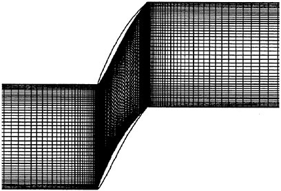
Figure 19 Blade to Blade Mesh
5.2 Propulsion Predictions
The predicted propulsive performance curves for model and full scale propellers are shown in Figure 20 for propeller C659 and Figure 21 for propeller C660.
At the design advance coefficient, for propeller C659, the full scale predicted thrust was 1.4% higher compared to that of the prediction for the model scale propeller. The torque coefficient was 3.1% higher for the full scale propeller compared with the model scale
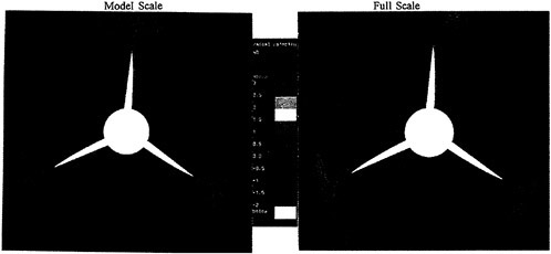
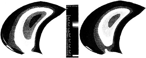
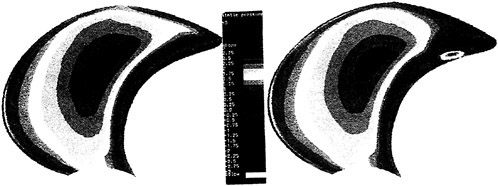
propeller, with a consequent reduction in efficiency.
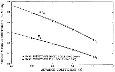
Figure 20 Propulsion Prediction for C659
For the second skewed propeller C660, at the same design coefficient, the full scale propeller produced 1% less thrust than the model scale propeller. This is attributed to the flow separation that is predicted for this propeller. The torque predictions for the full scale propeller were 0.3% higher that those of the model scale propeller.
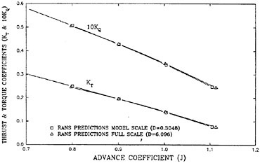
Figure 21 Propulsion Prediction for C660
In the study, at off-design conditions, the effect of propeller scale for the 5 blade propeller is significantly less than that of the 3 blade propeller. It is hypothesised that the scale effect has its maximum effect for the vortex flow structure. In that case the three blade propeller by having a much stronger tip vortex, due to the number of blades and the radial blade loading, will exhibit a greater scale effect for the propulsion predictions.
5.3 Static Pressure Predictions
Blade surface static pressure predictions have been made at one advance coefficient of J=0.8. It should be noted that at this off-design advance coefficient neither of the two skewed propellers showed any significant scale effect on the propulsion predictions, in contrast with the 3 blade propeller.
The most notable feature of the predicted static pressure distributions on propeller C659 for both model and full scale is the region of high −Cp in the region of the leading edge and the hub (Figure 22). There are not significant scale effect on the suction blade surface static pressure distributions.
For the second 5 blade propeller (C660) there are significant scale effect on the blade suction static pressure. The region of high and low static pressure near the trailing edge in the tip region are associated with a flow separation. The skewed propeller has a boundary layer separation near the trailing edge of the propeller. The location of the separation is best estimated from the hook shape in the static pressure contours near the trailing edge of Figure 23. As the flow separates so the boundary layer thickens as the axial velocity is reduced and the static pressure increases. At the same time the centrifugal effect within the boundary layer starts to dominate the flow and the resulting flow is predominately radially outwards.
6 Conclusions
6.1 3 Blade Propeller Validation
-
The propulsive predictions produced by the RANS code compare well with the model test results.
-
The degree of mesh alignment with the wake field had a significant effect on the predictions of the wake field.
-
The upstream circumferentially averaged velocities show some differences between the predicted and measured values and this is considered to be associated with the modelling of the upstream fairing cone by a long constant radius cylinder.
-
The downstream circumferentially predicted velocities agree well with the measured ones and this is reflected in the closeness of the propulsive predictions.
-
The blade-to-blade and wake predictions, generally, agree well with the measured data.
6.2 3 Blade Propeller Scale Effect
-
The propulsive predictions for the full scale propeller show the scale effect when compared with the predictions for the model scale propeller. The scale effect is largest at off-design condition when the advance coefficient is less than the design value.
-
The full three dimensional nature of the flow around the propeller blades has been investigated. The flow results show the complex nature of the flow around a propeller blade including the boundary layer, blade wake region and the tip vortex flow in the tip region.
-
The scale effect is most noticeable in the region of the tip vortex flow for both static pressure and flow velocities. These scale effects account for the difference in propulsive performances between the model and full scale sized propellers.
6.3 5 Blade Propeller Scale Effect
-
The propulsive predictions produced by the RANS showed that scale effect was present in the propulsion prediction. This was particularly true for propeller C660 with a reduced thrust at the design condition.
-
The scale effects were most noticeable, for the skewed propeller C660, on the blade surface static pressure predictions. Also predicted was the formation of a boundary layer separation near the trailing edge of the full scale propeller that was not present at the model scale. These scale effects on blade surface static pressure predictions account for the difference in propulsive performances for the skewed propeller between the model and full scale.
Acknowledgements
The Author would like to thank the Staff of DERA Haslar for their help in compiling this paper, especially Dr. C.Jenkins.
(C) British Crown Copyright 1998/DERA
Published with the permission of the Controller of Her Britannic Majesty’s Stationery Office.
References
Denny S.B., 1968, “Cavitation and Open-Water Performance Tests of a Series of Propellers Designed by Lifting-Surface methods”, David W.Taylor Naval Ship Research and Development Center Report 2878, September.
Jessup S.D., 1989, “An Experimental Investigation of Viscous Aspects of Propeller Blade Flow”, Doctor of Philosophy Dissertation, The Catholic University of America, Washington, D.C.
Stanier M.J., 1992, “Design and Evaluation of New Propeller Blade Sections”, International STG Symposium on Propulsors and Cavitation, Hamburg, June.
Stanier M.J., 1994, “Propeller Blade Sections with Improved Cavitation Performance”, Proceedings NAV’94 Conference, October 5–7, National Central Library, Rome.
Notation
|
CP |
|
|
C0.7 |
Propeller Chord at r/R=0.7 (m) |
|
D |
Propeller Diameter (m) |
|
Re |
|
|
J |
|
|
KT |
|
|
KQ |
|
|
n |
Propeller Rotation Speed (rps) |
|
P |
Local Pressure (N/m2) |
|
P∞ |
Free Stream Pressure (N/m2) |
|
Pv |
Vapour Pressure (N/m2) |
|
Q |
Propeller Torque (Nm) |
|
R |
Propeller Radius (m) |
|
r |
Local Propeller Radius (m) |
|
r0.7 |
Propeller Radius at r/R=0.7 (m) |
|
T |
Propeller Thrust (N) |
|
V∞ |
Free Stream Velocity (m/s) |
|
Vx |
Axial Velocity Component (m/s) |
|
Vr |
Radial Velocity Component (m/s) |
|
Vt |
Tangential Velocity Component (m/s) |
|
Vrel |
Blade Section Relative Velocity Vrel=√[(V∞)2+(2πnr0.7)2] |
|
ρ |
Density of Water (Kg/m3) |
|
υ |
Kinematic Viscosity (m2/s) |
DISCUSSION
S.Brizzolara
Universita di Genova, Italy
I appreciate very much the very well presented and design oriented work.
I was impressed by the good prediction of the increasing of negative pressure in the tip vortex region of the DTRC 4119. This fact is experienced also in reality, and each cavitation tunnel has its own empirical formula to extrapolate tip vortex cavitation from model scale to full scale (MacCormick or other).
Do you think it will be possible to define new correlation formulas based on CFD calculations in the near future?
AUTHOR’S REPLY
The current use of the ‘RANS’ code at DERA is to predict the full scale performance directly and it is used in conjunction with model test and model to full scale correlation procedures. The use of full scale predictions in the design stage hopefully will lead to better propeller designs. With regard to the formulation of correlation procedures, based on CFD calculation, more correction between full scale propeller performance and predictions is needed to assure the full scale accuracy of the method. Since full scale trials of this type are both difficult and costly, such correction may have to be undertaken based on model scale flow validation only and an act of faith for the full scale predictions.
DISCUSSION
S.Jessup
Naval Surface Warfare Center, Carderock Division, USA
The author’s demonstration of the application of RANS solutions to practical propeller problems is greatly appreciated. The time has come to use advanced viscous codes for real design problems. Also, the inclusion of validation with data is completely appropriate and today, required.
When comparing tip vortex flows to propeller 4119 results, the adjustment of the vortex location, I believe, is proper. Overall wake contraction seems to be difficult to capture accurately enough to expect spatially accurate
near-tip results. Therefore, radial movement of the vortex solution is the only way to correlate the details of the result. I would comment that the differences between measured and predicted results are the largest anywhere shown, in Figure 13, the tangential velocity at 0.94R, even well away from the vortex, in the blade to blade passage. It should be noted that the tangential velocity is also related to the blade circulation, and propeller thrust. It is not clear that the discrepancies in circumferential average tangential velocity are consistent with the comparison of thrust coefficient. Further investi-gation of this component may point to why the tangential velocity, in general, does not match the experimental result. I would suggest to the author that full 3-d comparisons of the vortex structure may assist in diagnosing the discrepancies in this region of the flow.
The investigation of scale propeller effects is certainly one of the most important applications of the RANS code. I would like the author to explain in more detail how the grid was modified to perform the high Reynolds number calculations. One would expect the blade boundary layer to become much thinner, requiring the migration of the mesh closer to the wall.
The author, again, has demonstrated the use of RANS for design problems. We are also beginning to use the codes for design purposes, particularly in the calculation of tip vortex flows. A question we have is whether the near wake must be gridded to a sufficiently refined level to fully capture the downstream vortex structure. Our calculations have shown Cpmin to occur very close to or at the blade trailing edge. It would be most desirable to detail grid around the blade surface only, and not worry about extreme grid refinement in the downstream vortex, which requires iterative calculations and regridding. Can the author comment on this?
The full scale solution for propeller C660 indicating flow separation near the trailing edge around 0.85R is curious. The model scale solution is what would be expected. Unfortunately, full scale surface flow visualization is not common or possibly has never been performed, and is therefore out of our experience base. I would recommend further inspection of the solution to understand its cause.
A milestone in the use of CFD for design problems will be reached when the user has sufficient confidence in the calculations to make critical decisions based on those solutions, even when results may not pass all tests of intuition. Can the author reflect further on his experience using RANS in propeller design, and for instance, were your conclusions on scale effects on thrust used to impact changes to full scale propulsion hardware?
Concluding, I would like to thank the author for his contribution. The use of RANS in design should be promoted fully. The practical problems of gridding, computation times, and geometry handling must be addressed along with education on what analysis parameters are important. In this way CFD can be integrated effectively into the unfortunately, time limited design process.
AUTHOR’S REPLY
The author would like to thank Dr. Jessup for his kind comments. With regard to the meshing strategies I would refer to the reply to Dr. Uto discussion.
With regard to meshing the wake downstream of the propeller, previous mesh sensitivity studies have shown that the wake meshing strategy has little effect on the flow predictions through the propeller blade row provided that the propeller blade row is suitably meshed in detail. Therefore if the region of interest is close to the blade then there is no need to carry out wake meshing. It should be noted that the wake alignment strategy does not increase the cost of performing these calculations.
The flow separation predicted for the full scale propeller C660 is not unique and a similar separation prediction can be found, Stanier 1998. Further work is being currently undertaken to investigate this effect further and would appear at the present to be a geometry related phenomenon, of pitch, rake, skew and blade thickness.
In recent propeller designs, the RANS code calculations have been used to make propeller parameter selections, both at model and full scale and now form a standard part of the propeller design procedures at DERA, for advanced propeller design.
Reference
Stanier M.J., 1998, “Investigation into propeller skew using a ‘RANS’ code—Part 2: Scale effects,” International Shipbuilding progress, Vol. 45, No. 443, September 1998.
DISCUSSION
J.English
Consultant, United Kingdom
Over the last few years I have been fortunate to follow the progress of Mr Stanier’s work, using, I believe, some of the most powerful computers in the UK’s MoD. The most vivid recollections of our conversations concerned the problems of suitable mesh generation and the large differences found between the propeller thrusts and torques from panel methods compared with the RANS solutions. My questions to him were mostly concerned with how long it would be until further significant stages were reached in the quest for answers to straightforward practical questions that could make our dependence on physical modelling less than it currently is. It is pleasing to see, therefore, that some aspects of the fundamental questions concerning viscous scale effects have been answered, albeit in the idealistic conditions of near uniform inflow and the absence of cavitation. On the other hand it is disconcerting that it has taken so long to reach this position considering the gulf that remains between what has been attained and what we need to know. Does the author consider that these advanced calculation techniques will eventually make physical testing unnecessary or are they likely to remain complementary tools in support of the latter?
Some of the author’s results are most impressive, especially the pressures on the suction sides of the blades, the conditions in the wake close to the propeller and the comparison of the calculated and measured propulsion results, although there must be some concern about the apparent lack of resolution of the flow in the close vicinity of the tip vortices. How sensitive are the results in the downstream propeller wake to the mesh particulars and the size of the control volume and has the author checked on this by varying them? In this context do limitations arise from the capacity of the computer facilities at his disposal and perhaps the personnel working on the project with him? The author’s References suggests that he is working virtually alone internationally at this level of detail. Is this correct as far as he is aware? I notice the author refers to the “method of artificial compressibility” in calculating pressure fields. Is this because he is using a computer code developed for use in aerodynamics rather than liquids that are virtually incompressible? Does he eventually expect to include cavitation and the change of state from water to vapour in his work?
A curious finding is that whereas the 3 bladed straight propeller behaves as expected re scale effect, the 5 bladed skewed propeller does not, as the predicted efficiency of the full scale propeller is slightly less than that of the model. The author refers to the radial flow strengthening from the centrifugal effect when flow separation occurs in the vicinity of the trailing edge. This flow feature can be removed of course by reshaping the blades there; however, of much more importance in my opinion is the beneficial flow separation that occurs at the leading edge, the presence of which is fundamental to the production of the cavitating leading-edge vortex and the prevention of rotational, cavitating break-off passing over the blades, with the attendant reduction in vibration excitation from this source. I suggest it would have been most instructive if the author had devoted time to studying the details of this flow, especially in the blade planeform view and in planes normal to the leading-edge. I would be very interested to know, for example, the magnitude of the axial velocity in the core of a propeller leading edge vortex and how it varies with sweep back and radial load distribution. Presumably it is this effect which sweeps partially vaporised rotational flow into the slipstreams of propellers with high leading-edge sweepback, through the vortices along the leading-edge and via the tip vortices.
AUTHOR’S REPLY
The author would like to thank Dr. English for his support over the years and for his contribution to this discussion. The author is of the opinion that physical testing will always be required, since numerical modelling by definition is a simplification of a very complex, real world. The use of numerical methods can give an insight into the flow that can only be achieved by complex and costly experiments. The author uses this particular method in the design of high performance propellers, to allow the checking of detailed flow in uniform inflow before committing the design to model manufacture and tests in ship wake fields.
The predictions for the downstream velocity are sensitive to mesh orientation to the flow as shown in Figure 5. The blade passage flow is less sensitive in this region since the mesh is body fitted. Extensive mesh sensitivity studies have shown that provided the number of cells within the blade passage is sufficiently large (approximately half the current mesh nodes), the thrust and torque results are insensitive to mesh. To increase the resolution of the detailed flow downstream of the propeller would require increased mesh nodes and hence reduce the cell volumes. The volume of the region of the tip vortex is a small fraction of the domain volume. Increased computing can lead to a simple increase in the number of nodes used, but more effective use can be made by the use of more complex mesh structure such as unstructured mesh solver schemes.
It is regrettable that the author did not include a short review of this type of numerical method within this paper and would have indicated the small number of other groups active in this area.
The continuity equation for incompressible flows does not allow the pressure term to be directly obtained. Numerical schemes are required to both satisfy the continuity and to allow the evaluation of the pressure term. The method of artificial compressibility is one way of obtaining this requirement for steady converged flows.
There are a number of cavitation models that could be used with this type of numerical methods and have been applied to a number of nonpropeller geometries, including pumps. Since the code is steady state this would be akin to conducting uniform inflow cavitation tests. Since cavitation problems of interest usually involve unsteady propeller operating conditions, an unsteady (time accurate) solver would first be required.
The flow around propellers is complex and for skewed propellers the flow appears even more complex. Dr. English’s description of leading edge flow are an important characteristic of skewed propellers and should rightly be investigated further. The results for the skewed propeller with the separation show that significant unexpected scale effect can change the performance of skewed propellers; the propeller designer must be aware of this to prevent poor full scale performance.
DISCUSSION
S. Uto
Ship Research Institute, Japan
I would like to thank Dr. Stanier for his successful work. First, I would like to confirm the simulation condition. Did the author use the same grid or not for the different Reynolds number flow? Does the turbulent flow develop from the leading edge of the propeller or not?
My second question is how accurately the blade boundary layer flow and the tip vortex are simulated at the model Reynolds number, because that gives the basis for the scale effect study. Would the author compare the intensity of tip vortex and the blade boundary layer characteristics (displacement thickness distribution at 0.7R location, for example) with the experiment data?
My third question is about the scale effect of the blade boundary layer characteristics. The 3-bladed propeller has so simple a geometry that the boundary layer flow around the mid-span location can be treated approximately as the 2-dimensional flow. Would the author compare the differences of the displacement thickness and the local skin friction coefficient between the two Reynolds numbers with those by the simple analytical solution (for the boundary layer flow over the flat plate, for example)?
In modeling the scale effects of propulsion coefficients, changes of friction and pressure components are treated independently in the theoretical framework. It gives us useful information if the author would present the contribution of these two components in the scale effects of propulsion coefficients for three propellers. This is my last comment.
Finally I congratulate the author again for his excellent achievement.
AUTHOR’S REPLY
The author would like to thank Dr. Uto for his contribution to the discussion. The grid generation is based on geometric conditions and does not take Reynolds number directly into account. There are small differences in the grids due to grid space weighting. For the full scale propellers the turbulent flow develops from the leading edge
cell, for the model scale transition is specified at a fixed percentage of the blade chord.
The accuracy of boundary layer flow can in part be obtained from the comparison of predicted and measured wake flow variables. The comparisons suggested would be useful but at the present time these have not been undertaken.
Although the 3-bladed propeller has a simple geometry the flow over the blade surface is far from simple and the author questions the validity of a comparison with 2-dimensional flow as suggested by Dr. Uto.
The propulsion coefficients are made up from two components, one pressure, the other wall shear stress. The pressure term also includes the influence of viscosity due to the boundary layer thickness resulting in blade to blade blockage, one of the effects of the viscous boundary layer. For completeness a comparison with Euler and potential calculations may give a better indication of the effect of viscosity. The following tables give a breakdown of the two components and have been non-dimensionalized using the resultant component obtained from the RANS code.
Pressure and Blade Surface Viscous Forces
|
Propeller |
J |
δΚΤp/ΚT |
δΚTτ/ΚT |
δΚQp/KQ |
δΚQτ/KQ |
Size |
|
dtrc4119 |
0.84 |
1.015 |
−0.015 |
0.897 |
0.103 |
model |
|
dtrc4119 |
0.50 |
1.006 |
−0.006 |
0.956 |
0.044 |
model |
|
dtrc4119 |
1.13 |
1.148 |
−0.148 |
0.692 |
0.308 |
model |
|
dtrc4119 |
0.84 |
1.013 |
−0.0.13 |
0.906 |
0.094 |
full |
|
dtrc4119 |
0.5 |
1.004 |
−0.004 |
0.961 |
0.039 |
full |
|
dtrc4119 |
1.12 |
1.088 |
−0.088 |
0.722 |
0.278 |
full |
|
C660 |
— |
1.012 |
−0.012 |
0.911 |
0.089 |
model |
|
C660 |
— |
1.012 |
−0.012 |
0.910 |
0.090 |
full |
RANS and Euler Predictions
|
Propeller |
J |
(KT)EULER/(KT)RANS |
(KQ)EULER/(KQ)RANS |
Size |
|
dtrc4119 |
0.84 |
1.066 |
0.925 |
model |
|
dtrc4119 |
0.50 |
1.029 |
0.967 |
model |
|
dtrc4119 |
1.13 |
1.644 |
0.761 |
model |
|
dtrc4119 |
0.84 |
1.056 |
0.935 |
full |
|
dtrc4119 |
0.5 |
1.001 |
0.948 |
full |
|
dtrc4119 |
1.12 |
1.259 |
0.792 |
full |
|
C660 |
— |
1.170 |
1.032 |
model |
|
C660 |
— |
1.145 |
1.016 |
full |


