
Validation of Theoretical Methods for Ship Motions by Means of Experiment
M.Ohkusu (Kyushu University, Japan)
Abstract
Some of theoretical methods to predict wave-induced motion and wave load of ships running at forward speed in waves are reviewed. We focus on validation of those theories by means of detailed experimental data on hydrodynamic pressure on the hull surface and/or wave elevation close to the hull surface. Traditional experiments comparing the predicted ship motions and global hydrodynamic force with the measured neither demonstrate the advantage of the advanced theoretical methods nor pinpoint the deficiency of them. It is because the ship motion and the global hydrodynamic force are the result of plenty factors integrated and do not provide high grade information on hydrodynamics involved.
1. Introduction
Since the late 1980’s vigorous effort has been made by many research workers to develop rational theoretical methods for predicting wave-induced motion and wave loads of ships. Most of them are boundary integral methods based on rational analysis of the free surface flow including the nonlinear effect. Some of them will be reviewed in this article. They attempt rigorous analysis no matter how complicated their implementation and they are computationally involved. The final goal of those methods is to understand and simulate the seakeeping of ships moving at forward speed in high waves.
Despite such progress achieved in the theoretical methods, experiments on which their validity is to be tested remains classical; most of seakeeping experiments are the ship motion test and the forced motion test for the global hydrodynamic force. Those experiments provide only low grade information on hydrodynamics of ship-wave interaction. Advantage of the advanced theoretical methods over the primitive methods will not be fully displayed in comparison with the result of those experiment; both the former and the latter methods are often presented by many authors to predict the ship motion and the global load with rather adequate accuracy. Though the advanced methods may predict some nonlinear phenomena which the primitive theories can not do so, quantitative information of such phenomena will not be obtained on the ordinary ship motion test.
Hydrodynamically correct theory must be the theory that is able to account for the flow field, hydrodynamic pressure distribution and wave elevation around a body. We may say that they are more hydrodynamic phenomena than the resulting body motion and global force. The ship motion is an integrated effect with which a lot of factors not only hydrodynamical but also mechanical are involved; fine prediction of the ship motion is an outcome of the correct account of hydrodynamics of elementary process of ship-wave interaction. The global hydrodynamic force is also an integrated result of hydrodynamic pressure which does not directly reflect the hydrodynamics.
The present author’s proposal is that hydrodynamically advanced theory or method must be tested on ‘hydrodynamic’ experiment rather than the ship motion experiment or the global force experiment. Hydrodynamic experiment means the experiment to understand basic hydrodynamics of the ship-wave interaction such as the measurement of the distribution of hydrodynamic pressure on the ship surface or the measurement of the wave field around the ship. We readily understand implication of this type of experiment if we recall a big role of the flow visualization rather than the drag measurement played in the progress of hydrodynamics of the body-flow interaction. Of course flow visualization is impossible with a ship in waves. Measurement of the hydrodynamic pressure and the wave field will be substitutes for it.
Objective of this article is to investigate validity of the modelling of the flow in the theoretical methods for ship motions by hydrodynamic experiment. We may expect it will demonstrate the advantage of the rigorous analysis and pinpoint where they are to be improved if any.
Regrettably few experimental data meeting our requirement are available; only several examples are found and compared with the prediction of the theoretical methods. Actually no experiment has ever been attempted to exemplify quantitatively the non-
linear effect of seakeeping which some of the theoretical methods are able to predict. So the methods whose validation is investigated in this article against the experimental results are mostly linear ones. We have to wait for the future work to confirm validity of the most sophisticated results of the nonlinear theories.
2. Linear Theory I
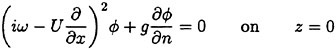
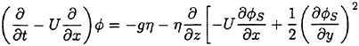
Correct modelling of the interaction of the steady disturbance on the water surface produced by the constant forward speed of a ship with the unsteady flow produced mainly by the ship-waves interaction is not straightforward in formulating a theoretical approach to predict the wave-induced motions and wave loads of the ship. The total flow produced by the ship in waves is obviously decomposed into the steady flow and the other flow naturally unsteady. It is appropriate to attempt the following form for the velocity potential Φ of the total flow.
(1)
The flow is described in the right-hand reference frame fixed to the ship moving at the constant speed U into the positive x direction; the x axis coincides with the ship’s center line and the x−y plane is the mean water surface; the z axis is taken vertically upward. The second term of (1) corresponds to the uniform flow relative to the ship, the third term ![]() represents the steady flow and the fourth term
represents the steady flow and the fourth term ![]() the unsteady flow component.
the unsteady flow component.
Wave elevation ζ is also a superposition of the steady component ηS and the unsteady component η.
(2)
Magnitude of the unsteady flow ![]() is determined by magnitude of the incident waves and the resulting ship motions. Magnitude of the steady flow
is determined by magnitude of the incident waves and the resulting ship motions. Magnitude of the steady flow ![]() is supposed to be dependent on ship geometry such as its slenderness. It means that rational basis of the linearization of
is supposed to be dependent on ship geometry such as its slenderness. It means that rational basis of the linearization of ![]() will be independent of that of
will be independent of that of ![]() . When we discuss their interaction without introducing any assumption on the ship geometry (practical hull forms are never slender), the most reasonable choice of
. When we discuss their interaction without introducing any assumption on the ship geometry (practical hull forms are never slender), the most reasonable choice of ![]() will be a full nonlinear solution. Yet we like to somehow avoid the full nonlinear solution and use physically correct but simpler solution; too complicated mathematical expression of
will be a full nonlinear solution. Yet we like to somehow avoid the full nonlinear solution and use physically correct but simpler solution; too complicated mathematical expression of ![]() might lead to unnecessary difficulty of any linear theory of the unsteady flow
might lead to unnecessary difficulty of any linear theory of the unsteady flow ![]() .
.
The choice of the steady flow model, if we have no mathematical basis, will inevitably be decided on physical argument or arbitrary; consequently various approaches will be possible to incorporate the effect of ![]() into
into ![]() . Their validity therefore must be carefully tested on ‘hydrodynamic’ experiment.
. Their validity therefore must be carefully tested on ‘hydrodynamic’ experiment.
A popular way to account for the steady flow effect allowing the relatively easy formulation of the unsteady flow is the introduction of the low order solution of the steady flow. The simplest choice is to assume the steady disturbance ![]() is zero; the steady flow around the ship is assumed to be only the uniform relative flow U in deriving the free surface conditions.
is zero; the steady flow around the ship is assumed to be only the uniform relative flow U in deriving the free surface conditions.
We linearize the free surface conditions and the hull surface condition, with respect to the velocity potential ![]() and the corresponding wave elevation η. The wave-induced ship motions are assumed to be of the order Ο (η).
and the corresponding wave elevation η. The wave-induced ship motions are assumed to be of the order Ο (η). ![]() will be a solution of the boundary value problem:
will be a solution of the boundary value problem:
(3)
(4)
(5)
(6)
and the radiation condition.
(4) and (5) are the free surface conditions satisfied on the mean water surface z=0. (6) is the body boundary condition imposed on SB representing the ship hull surface immersed under z=0 at the ship’s mean position, a is the motion vector of a point r(x, y, z) on the hull surface; r(x, y, z) moves due to the wave-induced ship motions. V is the steady flow velocity around the ship given by
(7)
n is the unit vector normal to the boundary surface and directing outward from the fluid. The third term of the body boundary condition on SB is to correct the difference of the steady flow velocity on SB from that on the exact instantaneous hull surface. The fourth compensates the effect of the variation Δn of
the unit normal vector n which is produced by the ship’s rotational motions (roll, pitch and yaw).
We have a computational problem when evaluating the right side of the body boundary condition (6). It includes the second derivative ![]() of which is singular at the corner on the hull surface and have to be carefully evaluated at the location of large curvature (Zhao and Faltinesen (1989)). In the time domain computation it might be better not to linearize the body boundary condition but to satisfy it on the exact instantaneous position of the body to avoid this problem though it is inconsistent.
of which is singular at the corner on the hull surface and have to be carefully evaluated at the location of large curvature (Zhao and Faltinesen (1989)). In the time domain computation it might be better not to linearize the body boundary condition but to satisfy it on the exact instantaneous position of the body to avoid this problem though it is inconsistent.
The body boundary condition (6) in this formulation might look strange because it includes the effect of ![]() notwithstanding we ignore it in the free surface conditions. Perhaps a consistent way is to neglect
notwithstanding we ignore it in the free surface conditions. Perhaps a consistent way is to neglect ![]() in the third and the fourth terms in (6). However it puts us in an uncomfortable situation: we feel the steady flow by the ship forward speed is never the relative uniform flow U even to the practically lowest order of approximation. To follow the formalism of the rational strip theory (Ogilvie and Tuck (1969)) will be a remedy for this. The rational strip theory claims consistently that the effect of
in the third and the fourth terms in (6). However it puts us in an uncomfortable situation: we feel the steady flow by the ship forward speed is never the relative uniform flow U even to the practically lowest order of approximation. To follow the formalism of the rational strip theory (Ogilvie and Tuck (1969)) will be a remedy for this. The rational strip theory claims consistently that the effect of ![]() is of higher order in the free surface condition, while it is not to be ignored in the body boundary condition. In this case, however, the choice of
is of higher order in the free surface condition, while it is not to be ignored in the body boundary condition. In this case, however, the choice of ![]() will return as a point in question.
will return as a point in question.
The Green’s second identity gives ![]() in the form
in the form
(8)
where r=(x, y, z) and r′=(x′, y′, z′). G is a function satisfying the Laplace equation and having a singularity of the form 1/|r−r′|. Integration of (8) is with respect to r′. SF represents the free surface (z=0 plane); S0 is a control surface surrounding the ship, located away from it and below z=0. If the field point r is located on one of the smooth boundary surfaces, 4π in the right side of equation (8) is replaced by 2π.
Hereafter in this section we concentrate on analysis in the frequency domain: the time dependency is in the form of eiωt as ![]() ηeiωt and aeiωt. Elimination of η from (4) and (5) yields
ηeiωt and aeiωt. Elimination of η from (4) and (5) yields
(9)
We substitute the Green function G0eiωt, which satisfies the free surface condition (9) and the radiation condition, for G in the equation (8). Then the equation (8) for ![]() on SB is transformed into
on SB is transformed into
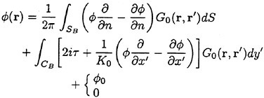
(10)
The first case is chosen when the incident wave of the wave number k
exists and otherwise the second case. CB is the intersection of SB and SF. K0=g/U2 and τ=ωU/g.
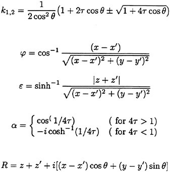
A key point tor implementing this approach is an efficient evaluation of the Green function G0. Iwashita and Ohkusu (1992) developed an efficient scheme to evaluate it numerically using a special mathematical expression by Bessho (1977).
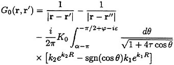
(11)
where r″=(x′, y′,−z′) and
The expression (11) of the Green function has several extraordinary features: it is straightforward
to control the accuracy of its numerical evaluation because (11) is a genuine single integral; it is analytically integrated over a panel over which ![]() is uniformly distributed (Iwashita and Ohkusu (1992)).
is uniformly distributed (Iwashita and Ohkusu (1992)).
The linear part of the unsteady hydrodynamic pressure Peiωt on the body wetted surface SB* at the exact instantaneous ship potion is evaluated by
(12)
All the functions in this equation are to be evaluated on the surface SB at the mean position of the ship. When computing the hydrodynamic force on the ship, Ρ must be multiplied by n+Δn and integrated on SB. The second parenthesis of (12) represents the restoring force in the generalized sense which is caused by the ship’s displacement in the nonuniform steady pressure field. It is independent of the unsteady flow ![]() because we know
because we know ![]() is not affected by
is not affected by ![]() . Therefore experimentally this term will be measured by prescribing a small steady displacement or rotation on a ship model during it runs on otherwise a calm water. Naturally the second line does not exist when the ship motion is suppressed. We notice that the first term in the second parenthesis, when we assume the wetted surface of SB is below z=0, will give the restoring force on calm water at zero forward speed.
. Therefore experimentally this term will be measured by prescribing a small steady displacement or rotation on a ship model during it runs on otherwise a calm water. Naturally the second line does not exist when the ship motion is suppressed. We notice that the first term in the second parenthesis, when we assume the wetted surface of SB is below z=0, will give the restoring force on calm water at zero forward speed.
The followings are a few points in question which arise when we implement this approach.
-
Choice of
 in (6) and (12) to evaluate V. Iwashita et al (1994) employed the double-model flow whose definition is given in the next section 3.
 -
The singularity associated with the intersection of SF and SB. Iwashita et al (1992, 1993, 1994) assumed
 on CB;
  is continuous at the intersection. They do not enforce the boundary condition exactly at the intersection but collocate at two points, one on SB and the other on SF which are very close to the intersection.
 -
Convergence of the solution as the size of the panels on SB approaches zero. SB is discretized into numerous quadrilateral panels over which
and its derivatives are approximated by a superposition of quadratic spline functions. Over each panel the product of the Green function and or its derivatives are numerically integrated. Convergence of their solutions is tested on increasing the panel numbers up to 2,000 (Iwashita et al. (1994)). Their conclusion is that 1,000 panels on SB will be sufficient on all the practical parameter values they are concerned and for ordinary hull forms; the computation will be extremely economical without sacrificing the accuracy by replacing the distribution with a single isolated G0 over each panel. They observed no instabilities in their numerical computations.
Finally we comment that similar approach to solve for ![]() in the time domain under the linear free surface conditions (4) and (5) is possible by employing the Green function in the time domain (King et al. (1989))
in the time domain under the linear free surface conditions (4) and (5) is possible by employing the Green function in the time domain (King et al. (1989))
Validation by Experiment
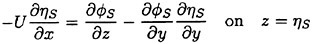
Validation of physical model assumed in a theoretical approach must be tested on ‘hydrodynamic’ experiment rather than ‘practical’ experiment. Even such a sophisticated theoretical approach as described in this section is often tested by comparing the prediction with the global hydrodynamic force and wave-induced ship motion measured at the towing tank. Such experiments are indeed ‘practically’ useful. However the global force is an integrated effect of hydrodynamic pressure on the ship and the ship motion is a result of a combined effect of many hydrodynamic factors. Fine agreement in the prediction of the ship motions does not necessarily allow us decide our theoretical approach is hydrodynamically correct; bad agreement does not let us know where the theory is wrong. More analytical experiment such as measurement of fluid pressure distribution and flow visualization will be necessary to prove their actual advantage or to pinpoint their inaccurate modelling.
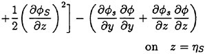
Results of extensive test for pressure distribution on a VLCC ship model (Cb=0.81, L/B=5.1) running in waves of various wave headings with its motion suppressed (diffraction problem) are reported (Iwashita et al. (1993)). Fig. 1, 2 and 3 are the results at the wave length-to-ship length ratio λ/L=0.5, Froude number Fn=0.2 and the wave height 0.02 of the ship length. Fig. 1 is amplitude of the pressure normalized by the amplitude of the incident wave at a section at St. No. 2, Fig. 2 at St. No. 5 and Fig. 3 at St. No. 9. The wave heading angle from 0° to 180° at upper to lower figures. The pressure is plotted vs azimuth angle measured anticlockwise from portside to starboard (−90° represents the the portside water line).
From the following to the head waves the agreement of the predicted (solid lines) with the measured (white circles) is excellent except for near the water surface at the bow section. It means the Green function method with uniform steady basis flow predicts well the wave pressure distribution on relatively blunt hull forms. This result is more than
we expected.
The discrepancy is very clear at the bow section. First of all, we remark that this would not be clear if we employed traditional way of experimental validation such as the comparison of the global wave exciting force on the ship. One obvious feature of the discrepancy is that the wave pressure at the bow section is extremely small on the water line at the ship’s mean position. Perhaps the pressure gauges at the water line will go out from the water periodically and it will record the zero pressure during this period. When the time series of the pressure thus recorded is Fourier analyzed, the amplitude of the fundamental frequency component must be very small compared with the amplitude obtained assuming a real sinusoidal temporal variation of the pressure as in the linear theory. It is not so serious problem because it depends on the definition of the pressure amplitude rather than the inaccuracy of the theory; if we compare the amplitude of the wave elevation instead of the pressure, we can avoid this ambiguity.
More serious discrepancy is that the measured pressure at the position a little below the water line is much larger than the predicted. If we are concerned with the vertical force on the ship, this inaccuracy in the theoretical prediction does not lead to serious practical problem: one of the reasons why a heuristic theory like the strip theory often appears to be valid. But from more hydrodynamical view point it will be a significant problem. Moreover the discrepancy will be practically serious when we are concerned with the local wave loads or added resistance of the ship.
No theoretical explanation is available at moment for the discrepancy. But the following guess is not unreasonable. Our physical model assumes the uniform flow as a basis flow. It is obviously not correct at the bow part; the flow must be deformed largely from the uniform flow at the bow part of blunt hull forms. So one remedy for improving theoretical prediction which occurs to us first is to introduce more accurate basis flow in the free surface condition (it will be described in the next section). At the station No. 9, where we observe the largest discrepancy, the steady wave surface is depressed lower than the mean water surface. On this steady surface the unsteady wave is superposed. Therefore the depth of a pressure gauge located close to the water line that is measured downward from the actual water surface is much shallower than the depth of the identical pressure gauge we assume in the linear theory, which is the depth measured from the surface of the unsteady
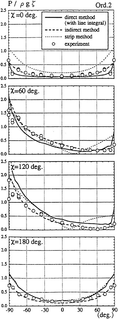
Fig. 1 Hydrodynamic pressure Fn=0.2, λ/L=0.5
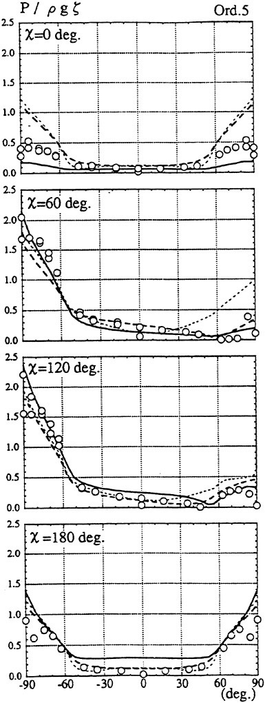
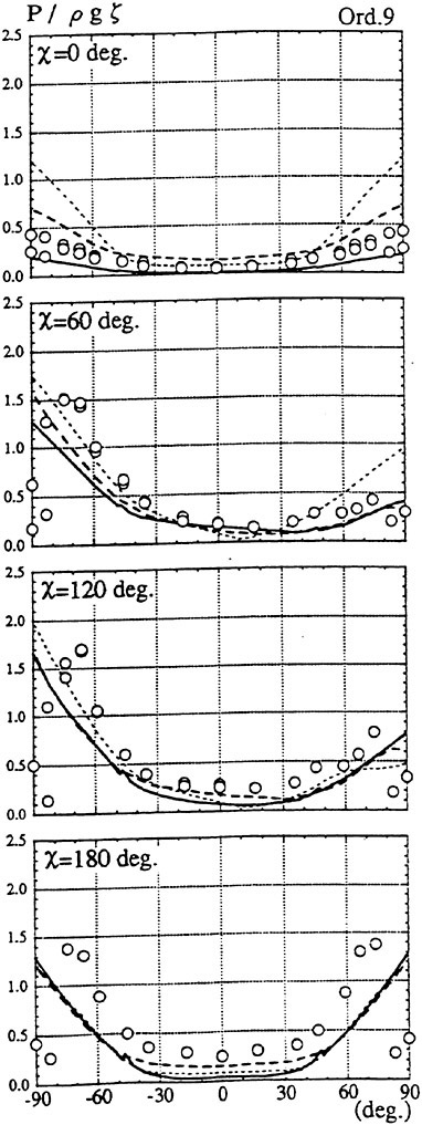
wave elevation superposed on z=0. The pressure gauge located actually shallower than we assume will record larger pressure than we predict in the linear theory. It implies that the effect of the steady wave elevation ηS must be taken into account in the prediction of the wave pressure at the bow part.
3. Linear Theory II
Inclusion of ![]() in the steady flow is more plausible when accounting for the steady flow effect on the free surface conditions for
in the steady flow is more plausible when accounting for the steady flow effect on the free surface conditions for ![]() if only we are able to find an appropriate
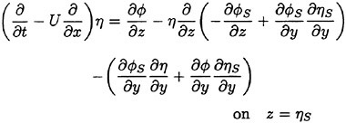
if only we are able to find an appropriate ![]() . We first write the complete free surface conditions:
. We first write the complete free surface conditions:
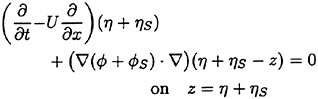
(13)
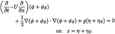
(14)
We are concerned with the unsteady part of the free surface conditions. We introduce an assumption for the steady flow ![]() explained later and linearize the free surface condition with respect to
explained later and linearize the free surface condition with respect to ![]() and η; we ignore the terms of
and η; we ignore the terms of ![]() Ο(η2) and the higher order. Then we have linearized free surface conditions for
Ο(η2) and the higher order. Then we have linearized free surface conditions for ![]()
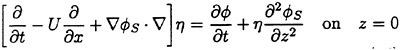
(15)
(16)
![]() , the steady flow which we employ in deriving (15) and (16), is the double body flow that satisfies the free surface condition
, the steady flow which we employ in deriving (15) and (16), is the double body flow that satisfies the free surface condition
(17)
Other assumptions are:
-
-
ηS is of higher order than
and the free surface condition is transferred from z=ηS to z=0
The assumption (i) implies that the steady flow and the steady wave elevation are much larger than the unsteady counterparts. The second (ii) will be valid if we assume the low forward speed of the ship. The steady wave elevation ηS of the flow satisfying (17) is given by
(18)
An assumption of very small U certainly leads to the higher order ηS which can be ignored. But now we do not employ such formalism on the consistency of the assumption. We just understand that the double model flow must be physically more plausible in accounting partly for the nonuniform steady flow dominating around ordinary hull forms which are not slender despite the assumption of ηS of the higher.
Linearization with respect to η admits transferring the body condition from the exact instantaneous hull surface under the water to the one at the mean position SB; the body condition is identical to (6). The velocity potential ![]() is written in the same form as the equation (8).
is written in the same form as the equation (8).
Mathematical expression of the Green function satisfying the free surface conditions (15) and (16), and the radiation condition will be extremely complicated even if it exists. So the so-called Rankine panel method employs a simple Rankine source function for G in the equation (8):
(19)
General idea of solving the integral equation (8) with the free surface conditions (15) and (16) is a time marching scheme starting with an appropriate initial condition. The free surface conditions (15) and (16) are used to update the velocity potential ![]() and the wave elevation η on SF (z=0). Solution of the ship motion equation provides the flux
and the wave elevation η on SF (z=0). Solution of the ship motion equation provides the flux ![]() over the hull surface SB.
over the hull surface SB.
The integral equation (8) with G given by (19) is solved numerically with respect to the unknowns ![]() over SF and
over SF and ![]() on SB with introduction of an appropriate radiation condition on S0. The radiation condition for the unsteady flow
on SB with introduction of an appropriate radiation condition on S0. The radiation condition for the unsteady flow ![]() is never given in an explicit form when the ship has a forward speed and implementation of this condition is, unless G itself satisfies it, not straightforward. We will discuss this problem later.
is never given in an explicit form when the ship has a forward speed and implementation of this condition is, unless G itself satisfies it, not straightforward. We will discuss this problem later.
Rankine panel method solving ![]() , particularly its numerical consistency and stability, has been systematically studied in both the frequency domain and
, particularly its numerical consistency and stability, has been systematically studied in both the frequency domain and
the time domain by Sclavounos and Nakos (1988), Nakos and Sclavounos (1990), Nakos et al. (1993), Vada and Nakos (1993), Kring (1994) and Kring et al. (1996). A fine review is given in Sclavounos (1996). In virtue of their investigation Rankine panel method is now one of the most reliable approach to find ![]() numerically based on the free surface conditions (15) and (16) or more general free surface conditions. We summarize their achievement and discuss some questions in the following:
numerically based on the free surface conditions (15) and (16) or more general free surface conditions. We summarize their achievement and discuss some questions in the following:
-
The boundary domain is discretized into plane quadrilateral panels, over which
 are approximated by a summation of bi-quadratic spline base functions.
 -
They used the so-called ‘empliciť Euler scheme (explicit for the integration of (15) and implicit for (16)) for time-marching integration of the free surface conditions. They studied systematically stability of this time marching scheme and reached the conclusion that the index Δx/Δt2 for lower U and Δx2/Δt3 for higher U must be larger than some critical value for the stable time marching integration. Here Δx is a spatial scale of the panels.
-
They found that discretizatin of the free surface, no matter how fine it is, distorts dispersive relation governing the wave propagation on the surface; the dispersive relation on the discretized free surface is different from that on the continuous free surface. It lets some wave components propagate into wrong direction. This analysis gives a consistency criterion which assures the convergence of the solution as each panel size approaches zero. The criterion is clearly stated in a relation of the panel aspect ratio, the panel Froude number and the reduced frequency in the frequency domain analysis.
A finite size of the panel causes another problem: aliasing of the energy of the waves with higher wave number than the Nyquist wave number π/Δx. It leads to spurious oscillation of the wave surface. They proposed a numerical filter to avoid the oscillation.
-
Radiation condition in their approach is enforced as a numerical wave absorbing beach away from the ship; the numerical wave absorbing beach is a layer of the free surface panels surrounding the free surface mesh and located distant from the ship. On this layer Rayleigh’s artificial viscosity type damping is introduced in the free surface condition. This idea was apparently successful after some numerical experiments. Yet it seems to require some know-how for this technique to succeed in developing robust scheme.
Condition of zero disturbance and zero wave slope in front of the ship works as a radiation condition for the case of Uω/g>0.25 if the analysis is in the frequency domain.
-
They do not mention how they treated with the singularity at intersection of the free surface and the hull surface. Our guess is that both the free surface condition and the hull surface condition are prescribed at the intersection as in the case at no forward speed (Dommermuth and Yue (1987)).
-
Integration of the equation of ship motions under the effect of hydrodynamic force must be done as a part of the time marching scheme of
in the time domain: the ship motions are determined by evaluated at a time step; the boundary value problem is solved with the updated ship motions to determine new and the resulting hydrodynamic force. The highest derivative of the equation of the ship motions is naturally the ship inertia term on the left side of it. The forcing terms (hydrodynamic force) too have implicitly acceleration-dependent part. Instability will occur in the numerical integration of such system. They avoided it by separating the hydrodynamic force into two parts: the instantaneous added mass part proportional to the instantaneous acceleration of the ship and the memory part dependent on the time history of the ship motion and velocity in the form of the convolution. The former part is transferred to the left of the equation to be combined into the inertia term; the remaining forcing term does not contain the acceleration dependence any more. Integration of this system is generally stable. It increases, however, the computing time because we have to evaluate two components of the hydrodynamic force separately.Instead of G of (19) we may use the Green function G0 (11). Hereafter we consider the problem in the frequency domain. We write the equation (8) with the Green function G0
(20)
where the choice of the last case depends upon if the incident wave exists or not. C0 is the intersection of SF and S0 at z=0. The integration on C0 is derived from the original integration on S0 by assuming ![]() vanishes on C0 because it is sufficiently distant from the ship and the double body flow
vanishes on C0 because it is sufficiently distant from the ship and the double body flow ![]() decays rapidly. We notice that the
decays rapidly. We notice that the ![]() of (20) satisfies the radiation condition because G0 satisfies it.
of (20) satisfies the radiation condition because G0 satisfies it.
The boundary domain is discretized into plane quadrilateral panels as in the case of Rankine panel method, over which ![]() are approximated by a superposition of bi-quadratic spline base functions. The integral equation (20), the body condition (6) prescribed on SB and the free surface conditions (15) and (16) with ∂/∂t replaced by iω will provide a system of linear equations on the unknowns.
are approximated by a superposition of bi-quadratic spline base functions. The integral equation (20), the body condition (6) prescribed on SB and the free surface conditions (15) and (16) with ∂/∂t replaced by iω will provide a system of linear equations on the unknowns.
In this formulation we do not need a special technique to numerically enforce the radiation condition. Instead a number of the unknowns on SF is more than that in Rankine panel method. Success of this approach will be dependent on the integration of the product of the Green function and ![]() on each panel of SF. A mathematical expression of the Green function proposed by Iwashita and Ohkusu (1991) may facilitate this integration.
on each panel of SF. A mathematical expression of the Green function proposed by Iwashita and Ohkusu (1991) may facilitate this integration.
Kashiwagi (1994) proceeds to an analytical transformation of the part of (19) to be integrated on SF. He reduces the number of the unknowns on SF by utilizing the free surface condition obtained after eliminating η from (15) and (16). This transformation increases the order of the derivatives of the functions to be evaluated on SF and the consequence is computational difficulty. His result is, however, mathematically significant. He proved a modified Haskind relation and the reciprocal relations on the hydrodynamic force which hold for ![]() on the double model flow
on the double model flow ![]() .
.
Other approaches to solve ![]() on the double model flow are: Yasukawa and Sakamoto (1991) introduces a special source function satisfying the free surface condition on the local flow
on the double model flow are: Yasukawa and Sakamoto (1991) introduces a special source function satisfying the free surface condition on the local flow ![]() for G in the equation (8). Takagi (1990) extends the radiation layer with damping, as used for the wave absorbing beach in Rankine panel method (for example Kring et al. (1994)), to the whole free surface but reduces the damping to the tuned limit. The former’s source function is mathematically complicated and use of G0 instead of their source function will be more plausible. In the latter the tuning of the damping has to be determined rather empirically and no theoretical method is available.
for G in the equation (8). Takagi (1990) extends the radiation layer with damping, as used for the wave absorbing beach in Rankine panel method (for example Kring et al. (1994)), to the whole free surface but reduces the damping to the tuned limit. The former’s source function is mathematically complicated and use of G0 instead of their source function will be more plausible. In the latter the tuning of the damping has to be determined rather empirically and no theoretical method is available.
Validation by Experiment
In section 2 we demonstrated that comparison of hydrodynamic pressure predicted and measured would be indeed the best way to investigate validity of the theories for hydrodynamic as well as practical viewpoint. Reliable experimental data of hydrodynamic pressure on the hull surface is not easy to obtain. Moreover how the measured pressure is to be compared with the predicted is sometimes ambiguous, particularly for the hydrodynamic pressure at a location which goes in and out the water during a period of the wave-induced ship motion. Observation of the wave elevation and comparison with the theoretical is easier in terms of experimental instrumentation and its accuracy is much more reliable than that of the measured fluid pressure. The wave elevation has close relationship with the pressure in the vicinity of the water surface and there is no ambiguity on what is to be compared with the predicted wave elevation.
We concentrate on the unsteady wave generated by a ship in the frequency domain. Actually the unsteady wave field generated by a ship translating at forward speed in waves is invisible at tank test because other waves such as the steady waves and the incident waves coexist. We need a technique to separate each of those waves. Another problem is that instantaneous distribution of the wave elevation around a ship model is not perfect data for the case of the unsteady wave η. A complete picture of η is obtained only after the spatial distribution of the amplitude and the phase is accurately measured. A technique was developed (Ohkusu and Wen (1996)) to overcome those difficulties and obtain the distribution of η around a ship model without a large number of wave probes installed.
Figs. 4, 5, 6 and 7 compare the theoretical wave elevation with the experimental one at ωt=0( cos component) and ωt=π/2 (sin component) at several x positions. Wave elevation is normalized by the amplitude of the incident wave and plotted vs y. A ship model is a Series-60, Cb=0.80 at the ballast condition. The model’s motions are restrained in head seas of the wave length to ship length ratio λ/L=0.5 and Froude number Fn is 0.20. The data shown in Figs. 4 to 7 are obtained by excluding the steady wave and the incident wave from η. The measured wave elevation plotted the most left in each of the figures is the wave elevation almost on the hull surface at the widest section of the ship; at the bow part the wave elevation is at the location little away from the hull surface (this is owing to the system of the wave measurement, see Ohkusu and Wen (1996)). Reason why we selected the ballast condition for the comparison is that we know the diffraction waves are higher than those at the full load condition particularly near the bow.
η is computed from ![]() , which is obtained by Rankine panel method assuming the double model flow in the free surface conditions, with
, which is obtained by Rankine panel method assuming the double model flow in the free surface conditions, with
(21)
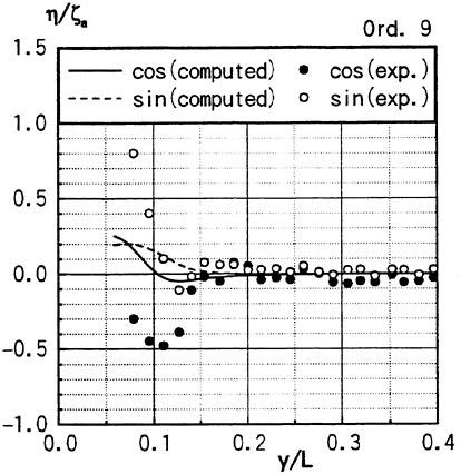
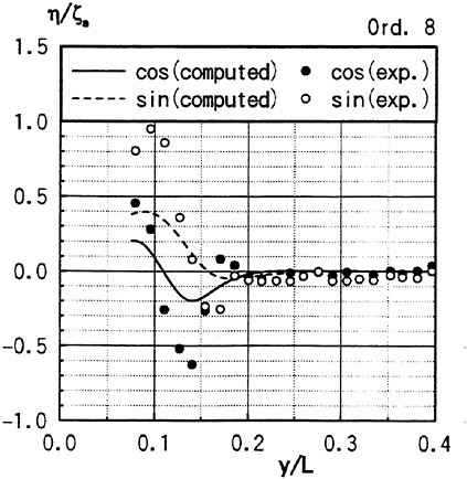
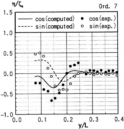
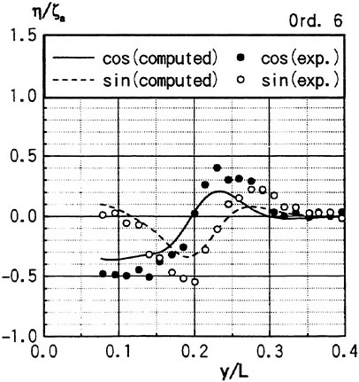
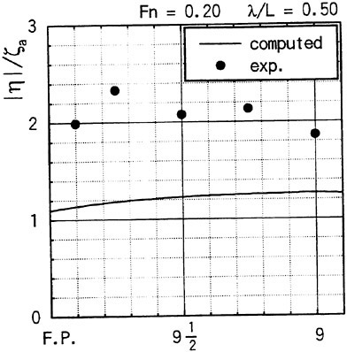
Fig. 8 Wave elevation along the hull surface
where ![]() stands for the gradient in the horizontal plane. The comparison of the computed η with the measured reveals the significant disagreement at St. No. 9 and 8. The measured wave height is considerably higher than the theoretical. However as we go away from the bow to downstream, the agreement is improved. At the midship zone the agreement is rather excellent. Conclusion is that taking
stands for the gradient in the horizontal plane. The comparison of the computed η with the measured reveals the significant disagreement at St. No. 9 and 8. The measured wave height is considerably higher than the theoretical. However as we go away from the bow to downstream, the agreement is improved. At the midship zone the agreement is rather excellent. Conclusion is that taking ![]() of the double model flow into our modelling does not improve the inaccuracy of the theory though the inaccuracy was reasoned due to the uniform steady flow assumption in section 2. A disappointing fact is that this three dimensional computation does not improve the prediction with a simpler ‘2.5 dimensional’ approach of the high speed slender body theory with the double model flow taken in the free surface condition (the results are not shown here).
of the double model flow into our modelling does not improve the inaccuracy of the theory though the inaccuracy was reasoned due to the uniform steady flow assumption in section 2. A disappointing fact is that this three dimensional computation does not improve the prediction with a simpler ‘2.5 dimensional’ approach of the high speed slender body theory with the double model flow taken in the free surface condition (the results are not shown here).
In order to confirm this conclusion we measured the wave elevation along the hull surface forward of St. No. 9 section and compare it with the theoretically predicted. Time series of the wave elevation is recorded by the capacitance type wave probe. Amplitude of the fundamental harmonics of the wave elevation thus recorded is plotted in Fig. 8. This value includes the effect of the incident waves. Reliability of this result is confirmed by other way (analysis of the video image). Discrepancy between the measured and the predicted is extreme but is expected from the difference we observe in Fig. 4.
4. Semi-Nonlinear Slender Body Theory
The steady wave elevation at the bow part is supposed to be high with high speed vessels and the effect of such high steady wave elevation must be significant on the unsteady flow at the bow part. We have shown already by two examples in section 2 and 3 that the steady wave elevation appears to dominate the accuracy of the wave pressure prediction at the bow part of even not high speed and not slender ships.
Full nonlinear theory must be our final goal but simpler approach capable to account for some of nonlinear features efficiently will be practically useful. Faltinsen and Zhao (1991) proposed an approach useful for high speed vessel and able to account for the effect of the steady wave elevation consistently. It is derived following Ogilvie’s bow flow model of the steady flow (Ogilvie (1972)).
Since high speed vessels are supposed to be of slender hull form, it is legitimate to introduce the slenderness parameter ε≪1. But we assume the slope of the hull form into the x direction is O(ε1/2) instead of Ο(ε). It sounds rather artificial but it is conceivable that the hull slope and therefore the flow quantity vary more rapidly of the order Ο(ε1/2) into the x direction at a part of the ship length, for example, at the bow part even if the hull form is globally slender of the order Ο(ε). Naturally x component of the unit normal n to the hull surface is Ο(ε1/2) and it follows that ![]() and ηS=Ο(ε). The former results from the body boundary condition and the latter is deduced from the steady wave elevation computed from
and ηS=Ο(ε). The former results from the body boundary condition and the latter is deduced from the steady wave elevation computed from ![]() . Variation of the flow will be
. Variation of the flow will be
in the fluid domain close to the hull surface. Here f represents a flow quantity we are concerned.
Under such assumptions we must not transfer the free surface condition from z=ηS to z=0 because they yield ηS∂/∂z=O(1). A model with the free surface condition to be satisfied on the steady wave surface will be likely to account for what the linear theories could not in the previous sections. Retaining the first order terms with respect to ![]() and η we write the free surface condition
and η we write the free surface condition
(22)
(23)
The governing equation for ![]() is two dimensional Laplace equation in the plane perpendicular to the x axis. The way to solve for
is two dimensional Laplace equation in the plane perpendicular to the x axis. The way to solve for ![]() is almost the same as an approach employed in Rankine panel method described in the previous section. The most time consuming part is two dimensional boundary value problem and computational burden is remarkably reduced.
is almost the same as an approach employed in Rankine panel method described in the previous section. The most time consuming part is two dimensional boundary value problem and computational burden is remarkably reduced.
The Green’s second identity applies to the fluid domain in a plane parallel to the y-z plane to yield an integral equation
(24)
In this equation CB is the contour of a cross section of the ship at x, CF the steady wave surface z=ηS and C0 the control surface at y=±Y for sufficiently large Y. r=(y, z) is the field point and r′=(y′, z′) is on the boundaries. θ(r′) is the angle between two tangents to the boundaries at x, this is naturally π for smooth curve.
With ![]() on the steady wave surface CF,
on the steady wave surface CF, ![]() on the body contour and the radiation condition on C0 prescribed, we solve numerically the integral equation (24): the boundaries are divided into segments over which
on the body contour and the radiation condition on C0 prescribed, we solve numerically the integral equation (24): the boundaries are divided into segments over which ![]() and its derivatives are approximated, for example, by spline functions. The free surface condition (22) and (23) controls the evolution of the
and its derivatives are approximated, for example, by spline functions. The free surface condition (22) and (23) controls the evolution of the ![]() and η on z=ηS along the characteristic line x+Ut=const; the condition (23) is used to forward the value of
and η on z=ηS along the characteristic line x+Ut=const; the condition (23) is used to forward the value of ![]() on z=ηS when the right hand side is known; the condition (24) updates the free surface elevation η at new (x, t). The body boundary condition prescribes the derivative of
on z=ηS when the right hand side is known; the condition (24) updates the free surface elevation η at new (x, t). The body boundary condition prescribes the derivative of ![]() into the normal direction on the contour of a cross section at new (x, t). This process is repeated starting from appropriate initial conditions until obtaining
into the normal direction on the contour of a cross section at new (x, t). This process is repeated starting from appropriate initial conditions until obtaining ![]() at every time instant and at every x.
at every time instant and at every x.
Radiation condition to be enforced on C0 is derived as follows: The steady flow ![]() and the wave elevation ηS will decay rapidly as |y| becomes larger; in the fluid domain out side C0 their effect will be ignored. The free surface condition there will be reduced to the ones on the uniform flow U to be satisfied on z=0. When is symmetrical
and the wave elevation ηS will decay rapidly as |y| becomes larger; in the fluid domain out side C0 their effect will be ignored. The free surface condition there will be reduced to the ones on the uniform flow U to be satisfied on z=0. When is symmetrical ![]() with respect to the x axis (head seas, heave and pitch motions),
with respect to the x axis (head seas, heave and pitch motions), ![]() , after the effect of the incident waves
, after the effect of the incident waves ![]() is excluded, will be at |y|>Y
is excluded, will be at |y|>Y
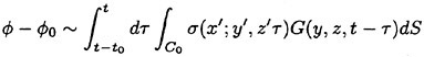
(25)
where t0=L/2U−x/U and x′=U(t−τ)+x. G is the well known time domain impulse function satisfying the linearized free surface condition.
(26)
G is written in the form
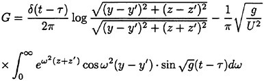
(27)
Some algebra yields an asymptotic form
(28)
Obviously ![]() given by (25) behaves the same way as (28) for
given by (25) behaves the same way as (28) for ![]() approaches to ∞. Derivation of the behavior of
approaches to ∞. Derivation of the behavior of ![]() at y±∞ for the asymmetric case is similar. Radiation condition we enforce at each sectional flow will be
at y±∞ for the asymmetric case is similar. Radiation condition we enforce at each sectional flow will be
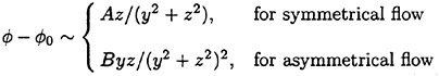
(29)
where A and B are constants.
Several other issues we should consider when implementing this approach are summarized below.
-
Evaluation of
and ηS. Similar approach to that for and η will work to solve and ηS under the free surface conditions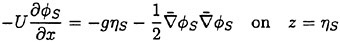
(30)
-
(31)
-
Implementation when the incident waves exist will not be straightforward. We formulate the problem for
 .
.  does not satisfy the free surface condition on z=ηS (
 actually satisfies the free surface condition on the uniform flow at z=0); the free surface conditions (22) and (23) for
  have some extra terms on their right side to make up for it. This means
  includes the diffraction of
  over the surface z=ηS as well as the diffraction by the ship.
 -
All the numerical results available are based on the same initial conditions of no disturbance in front of the ship. It will not be correct unless the ship form is really slender. It will be more so when we concerned with the deficiency of the flow prediction occurring at the bow part. Fontain and Faltinsen (1997) presents a new analysis of the flow in front of the bow intending to improve this defect for the steady flow case. We have no results available yet computed with this idea incorporated in the unsteady flow problem.
-
Main part of numerical computations in this approach is in two dimensional domain and it does not increase so much the load of computation to apply in the full nonlinear context, the full nonlinear free surface conditions and the body surface condition. However we are uncertain if the assumption of two dimensional flow is consistent with the full nonlinear free surface and body conditions. We doubt if the result is valid to the intended accuracy.
-
A confluence of the boundary conditions introduces a singularity at the intersection of CB and CF. Approach by Lin, Newman and Yue (1984) and Cointe (1987) will be a way to obtain realistic solutions. They prescribe both
and  at the intersection.
 -
This approach discretizes the evolution of the flow along a characteristic line. It is possible that this leads to a failure of consistency of numerical solutions, for example, the unintended distortion of the dispersive relation as pointed out in Rankine panel method (Nakos and Sclavounos (1990). But no investigation has been done along this line.
Validation by Experimental
Data of the experiment which meets our demand of testing the theoretical prediction hydrodynnamically are scarce. No data is available of hydrodynamic pressured with high speed vessels. Only data of the hydrodynamic experiment available are a few examples of the measured sectional force along the ship length.
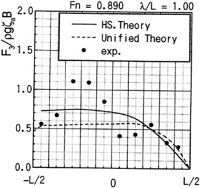
Fig. 9 Wave exciting force along the ship length
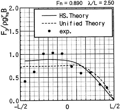
Fig. 10 Wave exciting force along the ship length
Th first example is the experiment of vertical hydrodynamic force on two ship models uniformly segmented along their length into ten parts. Experiment is on the wave force in the restrained condition and the total force when the ships are freely oscillating in waves (VTT (1994)). We compare the predicted sectional wave force in the vertical direction with the measured in Figs. 9 and 10 with a
slender hard chine model with a transom stern (CB=0.49, L/Β=9.96, Β/d=2.23 d: draft at mid-ship). The wave force was measured with the ship model restrained in head seas of the steepness 1/70.
Time series of the measured wave force on each segment are Fourier analyzed to obtain the amplitude of the fundamental harmonics component. The wave force per unit length of the ship is normalized by the amplitude of the incident waves and the ship breadth B. Fig. 9 is at Fn=0.89, λ/L=1.0 and Fig. 10 at Fn=0.89, λ/L=2.5. L/2 and −L/2 correspond to FP and Ap of the ship model. It is seen that the wave force fluctuates down the ship length and the fluctuation is harder for the shorter wave length. The solid lines represent the predicted by the slender body theory described in this section but with the free surface condition satisfied not on z=ηS but on z=0 and ![]() is a solution of the Neuman-Kelvin problem at the high speed slender body approximation.
is a solution of the Neuman-Kelvin problem at the high speed slender body approximation.
Agreement of the predicted and the measured is not bad at the bow part but the large fluctuation is not predicted. The tendency of less fluctuation at the longer wave length is very consistent in other results than the shown here and in any case the fluctuation almost disappears at the wave length of 5L. One conceivable reason of this disagreement is the effect of the steady wave elevation. To predict the wave force taking into account the effect of the finite steady wave elevation in the diffraction problem within the frame work of the high speed slender boy theory will be a future work
Keuning (1990) measured the sectional hydrodynamic force in the vertical direction on a ship model forced to heave or pitch motions. The model is towed on otherwise a cam water. Figs. 11 and 12 are reproduced from Faltinsen and Zhao (1991) where they compared Keuning’s results for the sectional added mass and damping computed with the computed by their method. The nonlinear steady free surface elevation was computed and incorporated into the free surface conditions of ![]() . In his original results Keuning (1990) represented the measured sectional coefficients by the bar notation to emphasize they are the average on each segment of the model. Here his results are plotted by black circles as the values at the middle of each segment. The sectional hydrodynamic force is supposed to vary smoothly in the x direction and Keuning’s average value will be the best fit to the value at the middle of each segment.
. In his original results Keuning (1990) represented the measured sectional coefficients by the bar notation to emphasize they are the average on each segment of the model. Here his results are plotted by black circles as the values at the middle of each segment. The sectional hydrodynamic force is supposed to vary smoothly in the x direction and Keuning’s average value will be the best fit to the value at the middle of each segment.
Agreement of the theoretical prediction by Faltinesen and Zhao (1991) with the measured is excellent. It tells that the correct consideration of the steady wave elevation will lead to the correct evalua
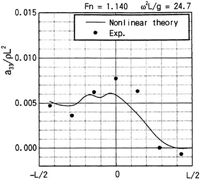
Fig. 11 Heave added mass along the ship length (Faltinsen and Zhao (1991))
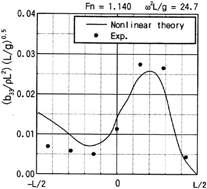
Fig. 12 Heave damping along the ship length (Faltinsen and Zhao (1991))
tion of the unsteady force even in details. We hope
measurement of the hydrodynamic pressure is attempted in future to confirm this more directly. We have tried several other methods which do not accurately model the steady wave elevation effect but without success.
We remark that there is a little ambiguity in the comparison stated above, Hydrodynamic pres-
sure given by (12) must be integrated on SB up to not z=0 but z=ηS in this case. Keuning’s result is obtained after excluding the restoring force on calm water. Therefore his sectional force includes the effect resulting from the integration of (a · ∇) (−ρgz) of (12) on SB from z=0 to z=ηS, which seems not to be included in the theoretical value by Faltinesen and Zhao (1991). It will affect the value of added mass when the ship model is not wall-sided. Discrepancy of added mass observed at the midship might be due to it because ηS is larger there. Restoring force transformed into the form of added mass is naturally the larger for the smaller ω.
5. Nonlinear Theories
A final goal for naval architects is to understand sea-keeping, wave-induced motions and loads, in severe sea conditions. We need a capability of analyzing the ship motion of large magnitude. Attempts into this direction are briefly described. We notice that the results of those attempts look promising but no systematic hydrodynamic experiment regrettably has been done to investigate their validity.
Body Nonlinear Theory
Lin and Yue (1991) proposed a three-dimensional time domain approach, where the body boundary condition is satisfied exactly on the instantaneous wetted surface of the moving body while the free surface conditions are linearized at its mean position. It is true that the body nonlinearity will affect the ship motions and wave loads to the large extent; a part of the ship hull will possibly go out from the water at severe sea state and it will not be appropriate if we solve the boundary value problem assuming that part is yet under the water. We remark that this type of approach was tried primitive way with the strip theory (Fukasawa (1990)). The result was claimed to agree with the measured in the time series of wave-induced loads such as bending moment. But it is based on too heuristic idea ignoring three dimensional effect but retaining the finite amplitude effect.
In Lin and Yue (1991) we do not need formally decompose the steady flow and the unsteady wave-induced flow any more. They analyze the problem in the earth-fixed reference frame in which the body boundary is moving. The forward translation of the ship is considered as a ‘large-magnitude’ motion in the earth-fixed reference frame. Good news with this way is that we need not bother the evaluation of the second derivatives of ![]() any more.
any more.
At each time instant the flow is described by a transient free-surface Green function source distribution on the instantaneous wetted body surface. The distribution is numerically determined by any appropriate technique described often in the previous sections. This Green function satisfies a linearized time domain free surface condition at z=0; the problem is considered in the earth-fixed reference frame, and therefore the Green function is the identical one as we use for the body motions at zero forward speed.
Efficient way (for example Newman (1985)) to evaluate the Green function and its derivatives will be a key for the success of this approach because the convolution integrals to be evaluated a plenty of times is the most time consuming task. Novel approach proposed recently by Clement (1998) will be one way to improve more the efficiency.
When the body doing the large amplitude motion we have to evaluate ![]() for hydrodynamic pressure on the body surface with a backward difference scheme. We can avoid to evaluate
for hydrodynamic pressure on the body surface with a backward difference scheme. We can avoid to evaluate ![]() by computing it via the material derivative. This technique works well for the prescribed motion of the body but it does not always give stable results for the integration of the free ship motions in waves. An alternative will be to solve boundary value problem for the Eulerian derivative
by computing it via the material derivative. This technique works well for the prescribed motion of the body but it does not always give stable results for the integration of the free ship motions in waves. An alternative will be to solve boundary value problem for the Eulerian derivative ![]() directly (van Daalen (1993), Tanizawa (1995)).
directly (van Daalen (1993), Tanizawa (1995)).
Wen (1997) employed this technique to evaluate successfully hydrodynamic pressure when he analyzed high speed ship motions of large amplitude with the high speed slender body theory described in section 4. No definite conclusion on this approach is possible now because no results for three dimensional problem are available.
Weak Scatterer Hypothesis
We encounter a non-realistic situation in the body nonlinear analysis when assuming the linear free surface conditions at z=0. On this assumption a part of the ship will be sometime above z=0 due to large motion and no hydrodynamic force will act on it. But in reality that part will be under the wave surface. In addition our observations of the interaction of the ship with steep incident waves in the towing tank suggests the magnitude of the ship wave disturbance is small compared with the magnitude of the incident waves. A consequence of this consideration is the so-called weak scatterer hypothesis (Pawlovski (1992)); the free surface condition is satisfied on the known incident wave surface.
Inclusion of the effect of ![]() in the free surface condition to be satisfied on the incident wave
in the free surface condition to be satisfied on the incident wave
surface makes the mathematical expression extremely complicated. Kring et al. (1996) implemented this approach together incorporating the body nonlinear condition. They compared their prediction of heave and pitch with the experimental data. But as mentioned often in this report such practical experiment as the ship motion test does not demonstrate the great benefit of this approach. We have wait for more hydrodynamic and systematic experiment done in future.
Fully Nonlinear Computation
most methods in time domain described above have to solve the boundary integral equation at each time step; the body nonlinear approach imposes the body boundary condition on the moving body surface but the free surface condition on the fixed plane z=0. It seems, however, not computationally a big jump from this to fully nonlinear approach. The difference is only to satisfy the free surface condition on the moving surface.
Beck et al (1994) and Scorpio (1997) are examples of the fully nonlinear computation. Their approach is:
-
The problem is solved within a limited fluid domain; the domain is truncated in the y direction by the solid wall which reflects back the wave energy. This must correspond to experiment in the towing tank. They assume the disturbance of the flow by the ship does not go far in from of the ship. It implies they are concerned with the relatively high speed τ>1/4
-
As usual we discretize the free surface into a number of panels. A mixed boundary value problem is solved at a fixed time instant with the boundary conditions
 prescribed on the instantaneous wetted body surface and given on the instantaneous free surface. We track the nodes on the free surface. The full non linear free surface conditions (13) and (14) are used to update the position of the free surface and the velocity potential at next time instant; naturally we do not decompose them into the steady and the unsteady ones.
 -
The boundary integral equation is in principle the same as (8) except that SF and SB move in time. Beck et al (1994) and Scorpio (1997) used the expression given by the distribution of Rankine source instead of (9). Rankine source replaces G. Their original way is to move the integration surface of the integral equation slightly off the control surface both on the body and the free surface to avoid singular kernel integration.
-
Another original technique is to track the node points on the free surface prescribing artificial horizontal velocity. If they are allowed to convect freely they will come to prohibited locations like inside the body and concentrate near a locations, which will cause large inconvenience and instability of the computations.
-
The propagation of the incident wave generated by wave maker in the towing tank is numerically simulated in advance. The velocity potential, its derivatives and the wave elevation at the truncation boundary located far upstream of the ship are used as the boundary condition when the ship-wave interaction is computed. It is legitimate because no disturbance is assumed to reach there.
Their method predicts the very steep wave elevation at the bow part of a ship model (a modified Wigley model) in head seas; it looks very realistic. It is the present author’s regret that no experiment to confirm the nonlinear effect predicted with their method has been attempted.
It will be crucial to validate carefully the numerical scheme in such complicated nonlinear computation including the desingularization technique; a good model of of the validation is that for Rankine panel method described in section 2. The work along this line is highly encouraged.
6. Concluding Remarks
Validity of three theoretical methods to predict the wave-induced motion and loads of ships at forward speed is tested by means of hydrodynamic experiment. They pass this strict test mostly. However it is shown that hydrodynamic pressure and wave elevation produced by the ship-wave interaction are not correctly predicted close to the ship’s front part. Reason of this deficiency appears to be neglect of the effect of the steady wave elevation dominating at the front part. Significant improvement of their validity will be expected to result from inclusion of the effect of the steady wave elevation into the free surface and the body conditions.
Acknowledgment
The author is pleased to acknowledge the assistance of Prof. H.Iwashita, Hiroshima University and Prof. M. Kashiwagi, Kyushu University in numerical computations.
References
Beck R F, Cao Y, Scorpio S M and Shultz W W (1994) Nonlinear ship motion computation using the desingularized method, Proc. 20th Symp. Naval Hydro. Santa Barbara
Bessho M (1977) On the fundamental singularity in a theory of motions in a seaway, Memoirs of the Defence Academy, Japan xvii/8
Clement A H (1998) An ordinary differential equations for the Green function of time domain free surface hydrodynamics, J. Eng. Math.
Cointe R, Molin B and Nays P (1988) Nonlinear and second order transient waves in a rectangular tank, proc. BOSS’88, Trondheim
Cointe R (1987) Remarks on the numerical treatment of the intersection point between a rigid body and a free surface, 3rd Workshop on Water Waves and Floating Bodies, Woodshole
Dommermuth D and Yue D K (1987) Numerical simulations of nonlinear axisymmetric flows with a free surface J. Fluid Mechanics vol. 178
Faltinsen O and Zhao R (1991) Numerical predictions of ship motions at high forward speed, Phil. Trans. Royal Soc. Lond. A 334
Fukasawa T (1990) On the numerical time integration method of nonlinear equation for ship motions and wave loads in oblique waves, J. Soc. Naval Arch. Japan, Vol. 167
Iwashita H, Ito A, Okada T, Ohkusu M, Takaki M and Mizoguchi S (1992) Wave forces acting on a blunt ship with forward speed in oblique sea, T. Soc. Naval. Arch. Japan, vol. 171
Iwashita H, Ito A, Okada T, Ohkusu M, Takaki M and Mizoguchi S (1993) Wave forces acting on a blunt ship with forward speed in oblique sea (2), T. Soc. Naval. Arch. Japan, vol. 173
Iwashita H, Ito A, Okada T, Ohkusu M, Takaki M and Mizoguchi S (1994) Wave forces acting on a blunt ship with forward speed in oblique sea (3), T. Soc. Naval. Arch. Japan, vol. 176
Iwashita H and Ohkusu M (1992) Green function method for ship motions at forward speed, Ship Technology Research, vol. 39
Kashiwagi M (1994) A new Green function method for the 3D unsteady problem of a ship at forward speed, Proc. 9th Workshop Water Waves Floating Bodies, Kuju
Keuning J A (1990) Distribution of added mass and damping along the length of a ship model moving at high forward speed, Int. Shipbuilding Progress 37, no. 410
King Β Κ, beck R F and Magee A R (1989) Sea-keeping calculations with forward speed using time-domain analysis, Proc. 11th Symp. naval hydro., Den Hague
Kring D C (1994) Time domain ship motions by a three dimensional rankine panel method, PhD Thesis, MIT
Kring D C and Sclavounos P D (1995) Numerical stability analysis for time domain ship motion simulations, J. Ship Research Vol. 39
Kring D, Huang Y F, Sclavounos P, Vada T and Braathen A (1996) Nonlinear ship motions and wave-induced loads by a Rankine method, 21st Symp. Naval Hydrdo. Trondheim
Lin W M, Newman N and Yue D K (1984) Proc. 15th Symp. Naval Hydro, Hamburg
Lin, W M and Yue D (1991) Numerical solutions for large-amplitude ship motions in the time domain, 18th Symp. Naval. Hydro. Ann Arbor, Michigan
Nakos D E and Sclavounos P D (1990) Steady and unsteady ship wave patterns, J. Fluid mechanics vol. 215
Nakos D E, Kring D C and Sclavounos P D (1993) Rankine panel methods for transient free surface flows, Proc. 6th Intl. Conf. on Numerical Ship Hydro, Iowa City
Newman J N (1985) The evaluation of free surface Green functions, Proc. Intl. Conf. Num. Ship. Hydro. Washington DC
Ogilvie T F and Tuck E O (1969) A rational strip theory of ship motions I, Rep. 13, Dept. Naval Archt. Marine. Eng. U. of Michigan
Ogilvie T F (1972) The wave generated by a fine ship bow, 9th Symp. Naval Hydro. Paris
Ohkusu M and Wen, G C (1996) radiation and diffraction waves of a ship at forward speed, Proc. 21st Symp. Naval. Hydro., Trondheim
Pawlovski J (1992) A nonlinear theory of ship motion in waves, Proc.. 19th Symp. Naval. Hydrdo. Seoul
Sclavounos P D (1996) Computation of wave ship interaction, Advances in Marine Hydrodynamics edited by M Ohkusu, Computational Mechanics Publication UK
Scorpio S M (1997) Fully nonlinear ship-wave computations using a multipole accelerated, desingularized method, PhD thesis, Univ of Michigan
Takagi K (1990) An application of Rankine source method for unsteady free surface flow, J. Kansai Soc Naval Arch. Japan vol. 213
Tanizawa K (1995) A nonlinear simulation method of 3-D body motions in waves (1st Report), T. Soc. Naval. Arch. Japan vol. 178
Vada T and Nakos D E (1993) Time marching schemes for ship motion simulations, Proc. 8th Workshop Water Waves and Floating Bodies
van Daalen E F G (1993) Numerical and theoretical studies of water waves and floating bodies, PhD thesis, Univ. Twente
VTT (1994) Wave loads on two fast monohull models, Research Rept. vol 22002/94/LAI, VTT, Finland
Wen G C (1997) Theoretical prediction of seakeeping of high speed ships, PhD Thesis, Kyushu Univ.
Yasukawa H and Sakamoto T (1991) A theoretical study on a free surface flow around slowly moving full hull forms in short waves, T. Soc. naval. Arch. japan vol. 170
Zhao R and Faltinsen O (1989) A discussion of the m-terms in the wave body interaction problem, Proc. 4th Workshop Water Waves and Floating Bodies, Oaystese
Extreme Rolling, Broaching, and Capsizing—Model Tests and Simulations of a Steered Ship in Waves
J.de Kat (Maritime Research Institute, The Netherlands)
W.Thomas III (Naval Surface Warfare Center, Carderock Division, USA)
ABSTRACT
The objective of this paper is to present recent research on the motions of a steered frigate-type hull in waves of moderate to extreme steepness. The paper describes model testing techniques, test data and some comparisons with numerical simulations related to large amplitude rolling, surfriding, broaching and capsizing in following to beam waves. To identify critical conditions, the investigation focuses on the combination of high speed and stern quartering (regular) waves for a frigate with a range of GM values. The role of non-linearities is discussed.
INTRODUCTION
As a sequel to the ship motions research reported by De Kat (1994), a second 4-year joint research effort on ship stability started in 1995 under sponsorship from the Cooperative Research Navies group. This CRNAV group, which comprises five navies (from Australia, Canada, Netherlands, United Kingdom and United States), U.S. Coast Guard and MARIN, focuses its current activities on the dynamic stability assessment of intact and damaged ships.
Modern naval ships have to satisfy stability criteria that are based on ship data from the 1930s, even though the underwater and upper hull forms have undergone major changes over the past 60 years. Using current knowledge and tools concerning ship motions, the objective is to evaluate ship stability in a more rational fashion; time domain simulations of ship motions in waves play a major role in this process.
Because of their intended use, the applied numerical tools should be subjected to proper verification and validation. The CRNAV group has an extensive database at its disposal with suitable seakeeping and manoeuvering data for intact ships. Validation data concerning extreme ship motions (including broaching and capsizing) are available to a very limited extent. To make the validation database more complete in terms of extreme conditions, tests were carried out in 1997 with a free-running frigate model.
This paper describes these model tests in detail, with the objective to provide insights into the physics of extreme motion events observed in the tests. The tests cover the most critical wave directions concerning dynamic stability during ship operations: following, stern quartering and beam seas were tested at different ship speeds with Froude number ranging from Fn=0.1 to 0.4. Extreme events include surfriding, broaching associated with surfriding, extreme rolling, and capsizing due to static loss of stability in a wave crest and due to dynamic loss of stability (coupled roll, yaw, surge, sway).
For a number of selected tests comparisons are made between measurements and time domain simulations. Simulations show the same trends as in the model tests concerning critical conditions—for an intact ship the combination of waves from astern (heading angle between 0 and 45 degrees) and relatively high speed is most dangerous. Even in the most onerous (minimum GM) condition, the ship did not capsize in beam waves.
MODEL TESTS
Model test data depicting capsizing, broaching and surfriding events are scarce in comparison with typical seakeeping data. Prior to the model test described in this paper, detailed capsizing model test data for frigate-vessels were available to the CRNAV group to a limited extent only. Thus, a model test program was undertaken for a frigate-type
hull form at high speeds in stern quartering seas. The model test program had two objectives:
-
To provide extreme motion data suitable for the validation of time domain ship motion predictions.
-
The comparison of a frigate’s ultimate stability behavior as a function of GM reduction in extreme conditions.
Fulfilment of the above objectives required the model tests to be carried out in a large basin capable of generating steep waves. A large test basin was required to maximize run length. The capability to generate steep waves allowed a test matrix to be developed, which would ensure the occurrence of extreme events, including capsizing, broaching and surfriding.
In addition to the tests in waves, the requirements included zigzag tests and roll decay tests at different speeds in calm water.
The matrix for tests in waves required:
-
High speed runs in beam seas through following seas of suitable run lengths to allow capsizing, broaching, and surfriding.
-
Large amplitude regular waves having typical steepnesses (Η/λ) of 1/20, 1/15, 1/10.
-
Wave length to ship length ratios (λ/L) between .75 and 2.50.
TEST BASIN
The capsize model tests and the calm water experiments were carried out in the Maneuvering and Seakeeping (MASK) Basin of the Carderock Division, Naval Surface Warfare Center. See Figure 1.
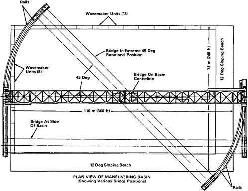
Figure 1. Maneuvering and Seakeeping Basin
The MASK is an indoor basin having an overall length of 110 m (360 ft), a width of 73 m (240 ft) and a depth of 6.1 m (20 ft) except for a 10.7 m (35 ft) wide trench parallel to the long side of the basin. The Basin is spanned by a 114.6 m (376 ft) bridge supported on a rail system that permits the bridge to transverse half the width of the basin and to rotate up to 45 degrees from the longitudinal centerline. Models can be tested at all headings relative to the waves. A 6.1 m (20 ft) wide by 6.6 m (21.8 ft) long by 2 m (6 ft) high towing carriage is hung from the bridge. The carriage has a maximum speed of 7.7 m/sec (15 knots) and is driven by a pair of opposing traction wheels driven by two electric motors through a worm gear drive.
MODEL DESCRIPTION
The model chosen for this study is a 1/36th scale fiberglass model of a frigate. See Figure 2. The 3 meter model was large enough for accurate seakeeping measurements, yet was small enough to take advantage of the steeper waves produced in the MASK. The hull form and skeg was constructed by the United States Naval Academy Hydromechanics Laboratory (NAHL) and was assigned the number 9096 by the Carderock Division, Naval Surface Warfare Center (CDNSWC).
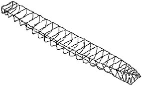
Figure 2. Isometric sketch of frigate (Model 9096)
The Seakeeping Department, Code 5500 of CDNSWC outfitted the model to be self-propelled using an autopilot for heading control. This autopilot uses a simple PID controller algorithm such that the desired rudder angle is:
(1)
where C1D is the yaw gain and C2D is the yaw rate gain.
The model was outfitted with bilge keels and twin rudders. Two four-bladed fixed pitch propellers (CDNSWC numbers 1991 and 1992) were installed on the model for inboard rotation.
A Plexiglas deck was installed to protect the instrumentation and machinery systems inside the hull from water damage during capsize events. The model was painted to enhance the display of the model during video recordings. See Figure 4.
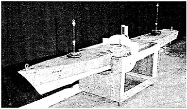
Figure 3. Outfitted model for capsize test
The outfitted model was tethered to the carriage by a cable bundle that contained control, power, and data signals. The cable was looped to minimize the effect of the cable tension on the model. The cable was connected to an overhead boom via a pulley that could be reeled in and out by a boom operator who stood on a platform mounted on the carriage. The boom could be yawed as desired by the boom operator. During the calm water and regular wave experiments, the carriage followed the model and the boom operator ensured that cable tension did not affect the model. The boom operator did this by pointing the boom so that it stayed above the model while reeling in or out the overhead pulley so that the cable remained slack. See Figure 4.
Figure 4. Model tether arrangement
INSTRUMENTATION
The carriage was equipped with a state-of-the-art Ship Motion Recording (SMR) system as developed by the CDNSWC Seakeeping Department. This system was connected to the sensors used in the model test as listed in Table 1 and described below.
The primary sensor used in the model test was a KEARFOTT T16 Miniature Integrated Land Navigation System (MILNAV™). This inertial navigation system (INS) included a monolithic 3-axis Ring Laser Gyroscope and three, single axis linear accelerometers. The MILNAV had the capability to measure extreme pitch, roll, and yaw angles, rates and accelerations. It was also used to determine surge, sway, and heave displacements, velocities, and accelerations near the center of gravity of the model. These motions were translated to the ships center of gravity reference for each load condition.).
Table 1. Capsize model test COLLECT Program data channels
|
Measurement |
Source |
|
Basin Wave Height From Carriage (cm) |
Sonic Transducer |
|
Basin Wave Height on shore (cm) |
Sonic Transducer |
|
Carriage Speed (m/s) |
Tachometer |
|
Propeller RPM (rev/minute) |
Tachometer |
|
INS Hull Speed (m/s) |
MILNAV™ |
|
INS Azimuth (°T) |
MILNAV™ |
|
Pitch (deg) |
MILNAV™ |
|
Pitch rate (deg/s) |
MILNAV™ |
|
Roll (deg) |
MILNAV™ |
|
Roll Rate (deg/s) |
MILNAV™ |
|
Yaw Rate (deg/s) |
MILNAV™ |
|
Rudder Angle (deg) |
Autopilot |
|
Rudder force, X direction (Newtons) |
Block Gauge |
|
Rudder Side force (Newton) |
Block Gauge |
|
Vertical Acceleration Forward (g) |
Accelerometer |
|
Longitudinal Acceleration Forward (g) |
Accelerometer |
|
Transverse Acceleration Forward (g) |
Accelerometer |
|
Vertical Acceleration Starboard (g) |
Accelerometer |
|
Longitudinal Acceleration Starboard (g) |
Accelerometer |
|
Transverse Acceleration Starboard (g) |
Accelerometer |
|
Relative Bow Motion, Port and Starboard (cm) |
Capacitance Probe |
|
Relative Stern Motion, Port and Starboard (cm) |
Capacitance Probe |
The accuracy of the yaw measurement was ±0.15°. Pitch and roll were measured with an accuracy of ±0.06°. Heave measurements had an accuracy of ±0.5%. Surge and Sway measurements had an accuracy of ±1%
Two triaxial accelerometers were used to measure accelerations. The first accelerometer package was placed at the bow center line of Station 2.0. The second accelerometer package was placed on the starboard side at station 10. The accuracy of the acceleration measurements were ±0.1%.
Model speed was measured using both the MILNAV™ inertial navigation system. Propeller speed was measured using a tachometer which was mounted to the propeller shafting. Propeller RPM as measured to ±1% accuracy.
Rudder angle was measured using the rudder feedback unit which as mechanically linked to the rudder tiller arm. The accuracy of the rudder feedback unit was ±3°.
Longitudinal and transverse rudder forces were measured using block gauges mounted on a free-floating plate that was attached to the rudder posts. The accuracy of the block gauge measurements of force was ±1%.
MODEL HYDROSTATICS
The model was tested in regular waves in stern quartering sees at three load configurations. The configurations tested included:
-
Full Load
-
Marginal GM condition
-
Failed GM condition
The load conditions were chosen with first priority given to the validation of the time domain simulation program FREDYN. Since the capsizing characteristics of the frigate were previously unknown, it was deemed necessary to choose 3 load conditions to ensure that capsizing would occur. As an additional consideration, it was desired that one load condition resemble a realistic operating condition of the ship. Thus, the first and most conservative condition tested closely resembled the typical frigate full load operating condition. The two remaining load conditions were achieved by the raising of weights above the deck of the model to reduce GM. This procedure ensured that displacement and freeboard remained constant amongst the three load conditions. Thus, the second load condition called “Marginal GM” represented a decrease in GM such that the model is in marginal
compliance with the U.S. Navy Criteria [2]. See Figure 5. The third load condition called “Failed GM” represented a load configuration that is in violation of the U.S. Navy Stability Criteria [2]; as such this is not a realistic operating condition.
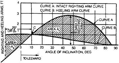
A summary of the full scale load configurations tested are presented in Table 2. The Ship Hull Characteristics Program (SHCP) program was used to confirm the model dimensions, draft, displacement, and GZ curve.
Table 2. Full Scale Load Conditions corresponding to model test
|
Parameter |
Load condition |
||
|
Full load |
Marginal GM |
Failed GM |
|
|
LPP (m) |
106.68 |
106.68 |
106.68 |
|
B (m) |
12.78 |
12.78 |
12.78 |
|
T (m) |
4.73 |
4.73 |
4.73 |
|
GMT (m) |
0.78 |
0.68 |
0.43 |
|
|
12.3 |
13.3 |
17.1 |
The transverse metacentric height (GMT) was measured prior to each run series in regular waves by conducting an inclining experiment. A ballast weight was successively shifted athwartships while the heel angle of the model was measured. From this information, the righting arm (GZ) was derived as a function of angle of heel. The transverse metacentric height (GMT) was derived from the slope of the GZ curve at the small angles of heel.
The roll, pitch and yaw gyradii (k44, k55 and k66) were determined using the pendulum method by swinging the model in the air. For each load condition, the model was suspended by a pivot located above the COG of the model and allowed to oscillate in e.g. pitch or roll. The gyradii were calculated from the respective oscillation periods.
TEST CONDITIONS
The model test matrix was designed for runs in regular waves for the three load (GM) conditions for the purpose of identifying critical, extreme motion situations, including capsizing, broaching, harmonic resonance and surfriding. Regular waves were chosen instead of irregular waves to allow a better understanding of observed extreme events in terms of known wave length, steepness, and phase relation with respect to the model; an important factor was the ability to use the data for validating a time domain simulation model.
The critical wave length range involved waves with λ/L between 0.75 and 2.50 with associated wave steepness in the range of 1/20 and 1/10. Model speeds were chosen between Fn_0=0.1 and 0.35 in combination with the selected wave and heading conditions. The critical wave headings chosen included following seas and stern quartering seas predominantly. Some runs were performed in beam seas.
Runs were performed at selected critical headings and speeds, which were based on time domain simulations carried out a priori. In case of the “Failed GM” loading condition, the occurrence of a capsize event invoked procedures that isolated the capsize region at the particular wave length λ/L. In general this meant that follow-up runs were made in higher and lower wave steepnesses and at lower (or higher) speeds until no capsizes were found. Adjacent headings were also tested at the capsize steepness to identify the effects of heading variations.
Table 3 provides an overview of the test runs for the ship with the Failed GM condition; χ represents the nominal heading angle. Test conditions for the other two loading conditions were in principle similar.
Table 3. Test matrix for Model 9096 in Failed GM condition (0 degrees is following seas)
|
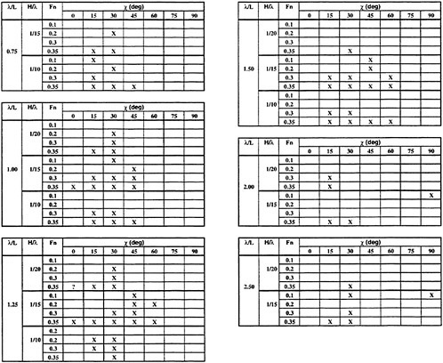 |
NUMERICAL SIMULATION MODEL
The numerical model was developed to simulate the large amplitude motions of a steered ship in severe seas and wind. The model consists of a nonlinear strip theory approach, where linear and nonlinear potential flow forces are added to maneuvering and viscous drag forces. The derivation of the equations of motions is based on the conservation of linear and angular momentum. These are given in principle in the inertial (earth-fixed) reference system, defined by the system of axes (xe,ye,ze). As the exciting forces are more easily described in the ship-fixed coordinate system, the Euler method is applied for deriving the equations of motion in terms of a rotating, ship-fixed coordinate system.
The equations of motion are given by:
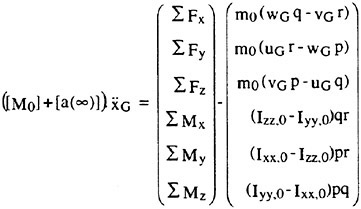
(2)
The matrix [M0] is the generalized (6×6) mass matrix of the intact ship, [a] is the added mass matrix containing the infinite frequency terms that are part of
the radiation forces (the convolution integrals are part of the RHS force terms); p, q and r represent the rotational velocities. The summation signs in the RHS represent the sum of all force and moment contributions, which result from:
-
Froude-Krylov force
-
Wave radiation (linear)
-
Diffraction (linear)
-
Viscous and maneuvering forces (non-linear)
-
Propeller thrust and hull resistance
-
Appendages (rudders, skeg, active fins)
-
When present: wind or internal fluid
Large angles are retained in the matrices for transformation between the ship-fixed and the earth-fixed coordinate system. The combination of the integrated static and dynamic pressures represents the total Froude-Krylov force (or moment), given by the vector:
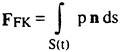
(3)
where n is the generalized normal vector and
(4)
S(t) represents the instantaneous wetted surface of the undisturbed, incoming wave with velocity potential Φl. Linear wave theory is used to describe the sea surface and wave kinematics.
Linear, 3-D transfer functions are used in the determination of the diffraction forces, and the wave radiation forces are based on linear retardation functions and convolution integrals (including forward speed terms). Viscous effects include roll damping due to hull and bilge keels, wave-induced drag due to wave orbital velocities, and non-linear maneuvering forces with empirically determined coefficients. The quasi-steady hull forces resulting from the motions in the horizontal plane consist of a linear and non-linear part:
(5)
where U and V are the time-dependent longitudinal and transverse velocity components, θ is the pitch angle, v(x,t) is the local transverse velocity at (sectional) location x, T(x,t) is the local draft, CDx is the local cross-flow drag coefficient, and ηt is the local wave orbital velocity in transverse direction. The roll moment resulting from lift and hull drag forces has the following nature:
(6)
The propeller thrust is estimated by:
(7)
where Np is the propeller RPM (assumed constant), KT is the thrust coefficient that depends on the instantaneous advance coefficient J, which depends on propeller diameter, RPM, ship speed U and wave orbital velocity ξt; tp is the thrust deduction coefficient at the propeller.
The hull resistance is based on the calm water characteristics as a function of instantaneous speed and sinkage. Appendage forces are estimated by using wing theory in the case of a rudder or active fin, and by using pressure drag in the case of a skeg. Interaction between rudder and hull is accounted for, and the instantaneous angle of attack depends on the ship motions, rudder angle, propeller race and local wave orbital velocities. The equations of motion are solved in the time domain using a 4th order Runge-Kutta scheme.
EXTREME MOTIONS AND CAPSIZING
The following provides a description of some extreme motion events, including:
-
Surfriding (and periodic surging)
-
Broaching
-
Extreme rolling
-
Capsizing
Surfriding
A ship in following seas can experience large speed fluctuations (at low encounter frequencies) about its mean forward speed. If the ship speed is sufficiently high, i.e. the speed that would be attained in calm water at a given propeller RPM and thrust, a wave may capture the ship and propel it at wave phase speed. The resulting speed can be significantly higher than the calm water speed.
Earlier work on Surfriding predictions (e.g. by Grim [3]) considered conditions leading to wave capture at phase speeds given by linear wave theory. More recent work (notably by Kan [4]) also takes into account non-linear effects on phase speed, which
leads to higher speeds for the steeper waves with a given period. The typical conjecture in surfriding research is that once captured by a wave, the ship attains a steady speed. An interesting result of the model tests presented here is that the ship can reach speeds well beyond the (steady) wave phase speed for an extended period.
To illustrate some of the results, we consider the frigate running in following seas (zero degrees heading angle) of different periods and heights. The loading condition corresponds to the Full Load case discussed above. At a calm water Froude number of Fn_0=0.3, the ship experiences periodic oscillations in forward speed; Figure 6 provides an overview of measured minimum and maximum speeds as a function of non-dimensional wavelength. For reference purposes in the figures presented in this paper, we use a definition for wavelength based on linear wave theory in deep water, i.e. λ=gT2/2π, where Τ is the period.
Figure 6 shows maximum and minimum speeds for different wave steepness values per wave period. The larger the wave steepness for a given wave period, the larger the speed fluctuation will be; the maximum wave steepness tested corresponds to approximately Η/λ=0.1 for each wave period considered. The minimum wave steepness represented is Η/λ=0.05. Cp_1 represents the phase speed according to linear wave theory, while Cp_5 is the phase speed determined according to Stokes 5th order theory (Fenton [5]); the phase speeds have been normalized by the square root of gL.
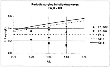
Figure 6. Measured (normalized) maximum and minimum ship speeds as a function of wavelength and wave steepness (Η/λ ranges from 0.05 to 0.1 per wave period). Cp_1 is the phase speed based on linear wave theory, Cp_5 is the phase speed based on Stokes 5th order theory for Η/λ=0.1
Figure 7 provides an example of measured and predicted time series for the case depicted in Figure 6 with λ/L=1.25 and Η/λ=0.05; Fn_0=0.3 corresponds to U=9.7 m/s. The numerical simulation model predicts the mean speed and the speed variation amplitude reasonably well. Figure 8 presents the same data, the only difference being a twice as high wave steepness, Η/λ=0.1. It is interesting to note that the simulation predicts steady surfriding (at linear phase speed), while this does not occur in the model test. This difference may be attributed to the higher wave phase speed in the model test, where the maximum ship speed is less than the actual phase speed, Cp_5, estimated by Stokes 5th order theory.
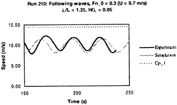
Figure 7. Measured and predicted speed in following waves
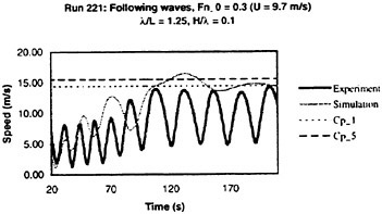
Figure 8. Measured and predicted ship speed in steep following waves
The model tests show that for the speed range Fn_0≤0.3 wave capture (and hence surfriding) does not occur in the wave conditions tested. For Fn_0=0.35 a drastic change in surge character occurs, for at this speed setting the frigate model does experience wave capture and surfriding events. In a number of tests where wave capture takes place in following waves, the ship is accelerated to a speed that lies well beyond the phase speed of the wave. Figure 9 provides an overview of measured maximum speeds for Fn_0=0.35 in the same format as for Figure 6. The maximum ship speed increases with
increasing wave steepness; for the conditions with λ/L=1 the steepness tested is Η/λ=0.077 and 0.097, while for λ/L=1.25 the steepness is Η/λ=0.051 and 0.092.
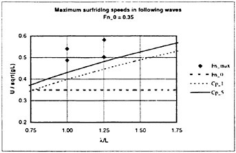
Figure 9. Maximum attained ship speed (Fn_max) following wave capture in experiments. Cp_1 is the phase velocity based on linear wave theory; Cp_5 is the phase velocity for Η/λ=0.1
Figure 9 shows that especially for the steepest waves, the maximum ship speed reaches very high values. The time series describe the character of this behavior, as shown for run 228 in Figure 10 for λ/L=1.0 and Η/λ=0.077. This figure shows that as the ship reaches a critical speed level in the model test, wave capture occurs and the ship accelerates to a speed beyond its calm water speed. The observed mechanism is as follows: at approximately t=140 s a wave crest reaches the stern of the ship and causes the ship to surge forward. At around t=150 s the crest has reached the aft quarter (i.e. it has overtaken the ship slowly until the ship speed equals the celerity), at which stage the ship is subjected to a large surge force. This causes the ship to accelerate and overtake the wave crest, which by t=170 s is situated at the stern again; the maximum speed is 15.8 m/s. While the ship accelerates and overtakes the wave crest, it buries the bow in the back slope of the preceding wave. The (complete) submergence of the bow increases the resistance and eventually causes the ship to decelerate; between t=170 s and 190 s the speed decreases to just below the wave celerity. As the crest overtakes the ship, the ship speed increases again to the wave celerity level.
The numerical simulation shows a similar behavior compared to the model test, but it predicts smaller speed fluctuations. Furthermore, as a consequence of the linear wave model, the surfriding speed is equal to the linear wave celerity (Cp_1), which lies below the actual wave speed, Cp_5.
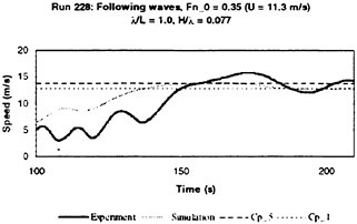
Figure 10. Measured and predicted ship speed during surfriding events for run 228
Figure 11 shows the effect of increased wave steepness in run 231 (Η/λ=0.097) when compared with Figure 10. In principle the same physical observations are applicable as for run 228 with the lower wave steepness; the variations in speed are much larger, however. The higher steepness leads to a maximum speed of 17.5 m/s; at this stage the bow is buried in the back slope of the wave to an even larger extent than in run 228. As a consequence, the speed drops to 11.9 m/s before accelerating again to wave celerity level. The numerical simulations predict speed fluctuations that exceed those for the lower wave steepness case in run 228, but the maximum simulated speed of 14.4 m/s lies well below the measured maximum speed.
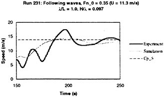
Figure 11. Measured and predicted ship speed during surfriding events for run 231
Kan [4] provides a procedure to estimate the critical (calm water) ship speed that will lead to steady surfriding as a function of wave and ship parameters; this method has been applied by Hamamoto et al [6]. So far, the issue of transient forward speed above the wave phase speed has not been addressed in detail. The issue is of relevance especially for irregular following seas, where steep waves will be able to push the ship speed to high
values for some time, with broaching as a possible consequence.
In the surfriding cases discussed above, the frigate stays on a course close to zero degrees; even though the bow of the ship is buried in the back of the wave slope during surfriding, broaching did not occur. Figures 12 and 13 show the measured roll, pitch and yaw angles for run 228 and 231, respectively.
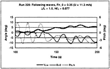
Figure 12. Measured roll, pitch and yaw angles for run 228
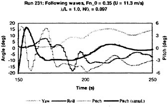
Figure 13. Measured roll, pitch and yaw angles for run 231, and predicted pitch
Broaching
The model tests show that the frigate investigated can experience broaching under certain conditions at high Froude number only (Fn_0=0.35). In general the ship proved to have good course keeping qualities in following and stern quartering waves, i.e. broaching did not occur frequently in the conditions tested at high Froude number. Two modes of broaching were observed:
-
Broach preceded by surfriding with steadily increasing heading deviation
-
Large amplitude, low-frequency yaw (heading) oscillations
Figures 14 and 15 depict the occurrence of the first broaching mode for the ship in the Marginal GM Condition. The nominal (desired) heading is 15 degrees. Figure 14 shows both the longitudinal and transverse ship speeds, where Us is defined in the horizontal plane along the x-axis of the yawed ship, and Vs is perpendicular to Us in the horizontal plane. Figure 15 shows the steadily increasing heading angle once the ship has been captured by the wave; the ship experiences moderately large heeling angles during the event. As a consequence of the test set-up, the broach ended when a tight tether line limited the motions.
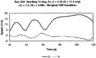
Figure 14. Mode 1 broach: Measured longitudinal and transverse ship speeds for run 324
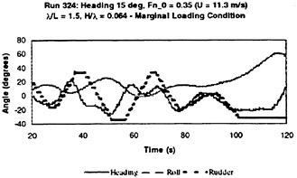
Figure 15. Mode 1 broach: Measured heading, roll and rudder angles for run 324
Figures 16 and 17 depict the occurrence of the second broaching mode for the ship in the Marginal GM Condition. Figure 16 shows that the ship has a significant mean negative drift velocity, i.e. it experiences a rather large drift speed to leeward while yawing. The highest transverse drift velocity occurs when the yaw angle (toward the wave) and forward speed increase while a wave crest is overtaking the ship (from aft to amidships). When the crest is in the midship area and the ship has reached its largest yaw deviation into the wave, the roll angle to leeward (negative sign) is largest; the reduction of the righting arm in the wave crest leads to asymmetric
roll motions. In this case the ship experiences large roll angles, but it does not capsize.
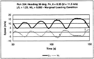
Figure 16. Mode 2 broach: Measured longitudinal and transverse ship speeds for run 354
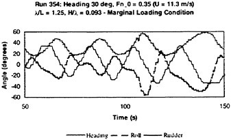
Figure 17. Mode 2 broach: Measured heading, roll and rudder angles for run 354
To illustrate that the ship can experience extreme roll angles also in the Full Load Condition, Figure 18 depicts the measured motions for run 252; the maximum roll angle (to port) is almost 60 degrees.
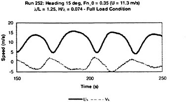
Figure 18. Mode 2 broach: Measured longitudinal and transverse ship speeds for run 252
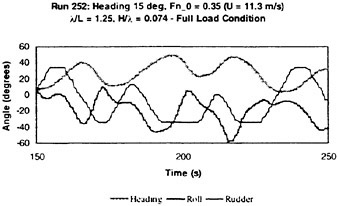
Figure 19. Mode 2 broach: Measured heading, roll and rudder angles for run 252
The stable course keeping properties of the frigate in waves may be linked to its degree of directional stability in calm water. Using the numerical model, pull-out tests were simulated and analyzed; Figure 20 shows the r-δ curve derived from these simulations at Fn=0.35 in calm water. This figure indicates that according to the simulations the ship is directionally very stable. The large skeg and twin rudders contribute to the frigate’s directional stability.
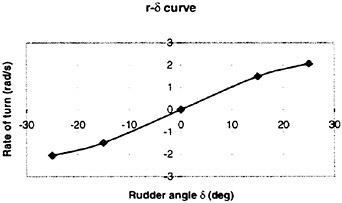
Figure 20. Calm water maneuvering characteristics derived from simulations for Fn=0.35 (Full Load Condition).
Capsizing
The frigate did not capsize under any of the speed, heading and wave combinations tested in either the Full Load or Marginal Loading Condition. In the Failed Loading Condition, however, capsizes did occur frequently at the highest ship speeds (Fn_0 ≥0.3) in following and stern quartering waves; no capsizes occurred at Fn_0<0.3, even though conditions included harmonic resonance in steep stern quartering and beam seas.
Three main modes of capsize could be distinguished from the experiments:
-
Loss of transverse stability in wave crest associated with surfriding or periodic surging
-
Dynamic loss of stability due to surge-roll-yaw coupling
-
Broaching (mode 2 with large yaw oscillations)
The majority of observed capsizes were of mode 1 and 2, which are described below in some detail. A mode 1 capsize is shown in Figures 21 and 22, where the ship capsizes while being overtaken slowly by a wave crest. For this capsize mode, typically the ship does not experience extreme roll motions before the final “half roll.”
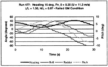
Figure 21. Mode 1 capsize: loss of stability in wave crest (run 477)

Figure 22. Ship velocities associated with mode 1 capsize (run 477)
A mode 2 capsize involves significant rolling, and often the roll motion tends to build up in severity before capsizing occurs. We illustrate this mode for three experimental cases: run 414 with a short wavelength ratio (λ/L=0.8), run 427 with λ/L =1.25, and run 448 with a relatively long wave (λ/L =2.5), as shown in Figures 23, 24 and 25, respectively. The motion behavior differs for these three cases: e.g. the speed variations in run 414 are limited to relatively small fluctuations about the mean forward speed, the roll motion in run 427 shows increasing extreme roll angles to port (negative sign, to leeward), and the roll motion in run 448 has a double period.
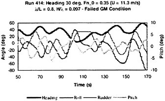
Figure 23a. Mode 2 capsize: dynamic loss of stability (run 414) with measured heading, roll, pitch and rudder angles
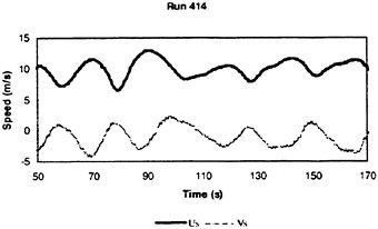
Figure 23b. Measured ship velocities associated with mode 2 capsize (run 414)
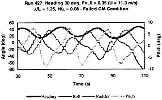
Figure 24a. Mode 2 capsize: dynamic loss of stability (run 427) with measured heading, roll, pitch and rudder angles
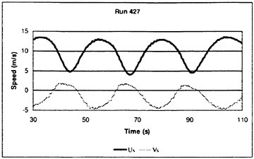
Figure 24b. Ship velocities associated with mode 2 capsize (run 427)
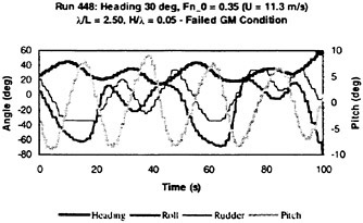
Figure 25a. Mode 2 capsize: dynamic loss of stability (run 448)
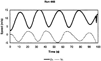
Figure 25b. Ship velocities associated with mode 2 capsize (run 448)
In these dynamic (mode 2) capsize events the ship capsizes typically in the wave crest.
INFLUENCE OF SHIP SPEED AND GM ON CAPSIZING
Ship speed has a major influence on capsize avoidance for a given set of conditions. Let us consider test run no. 421, which results in a capsize (mode 1) for the frigate with Failed GM condition at Fn_0=0.35 as shown in Figure 26. The capsize occurs during wave capture from the second wave where stability is completely lost in the wave crest. The wave conditions are: λ/L=1.0, nominal heading angle is 30 degrees and wave steepness is Η/λ=0.07.
The ship dynamics change drastically by reducing speed to Fn_0=0.3; run 420 illustrates that the reduction in speed increases the wave encounter frequency and hence decreases the duration of wave crest riding, see Figure 27. Stability is lost temporarily with the passing of each wave from astern, enough to submerge the deck edge, but the duration and magnitude of the degradation are not sufficient to cause a capsize event.
Run 337 represents the same run as run 421 with the exception that the ship is in the Marginal GM condition, see Figure 28. Waves slowly overtake the ship from the starboard quarter. Each passing wave captures the ship where a brief surfriding event takes place. The stability reduction experienced by the ship induces the ship to heel to port at a large angle of roll. As the ship is released by the wave, the ship rolls back to starboard and uprights itself in the wave trough. This cycle repeats with the next wave as it approaches slowly from the stern.
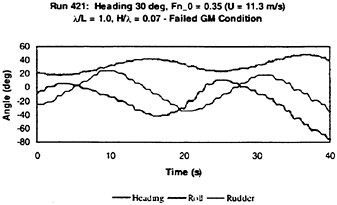
Figure 26. Run 421: Capsize for frigate with Failed GM condition, Fn=0.35
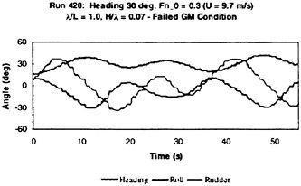
Figure 27. Run 420: Capsize (run 421) avoidance for Failed GM case by speed reduction to Fn=0.3
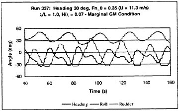
Figure 28. Run 337: Capsize (run 421) avoidance for Fn=0.35 by increased GM (Marginal condition, Fn=0.35)
DRIFT IN STERN QUARTERING WAVES
Analysis of the ship velocities in the horizontal plane for the tested stern quartering wave conditions shows that a ship can experience large speed fluctuations periodically in both forward and transverse directions. As a consequence, the instantaneous drift angles can be substantial. In addition, in such conditions a ship can experience a significant mean (sideways) drift velocity. To illustrate this aspect, we consider the velocity components Us and Vs associated with run 337. The instantaneous drift angle shown in Figure 29 is given by
(8)
i.e. this is the drift angle with respect to the yawed x-axis of the ship in the horizontal plane. Figure 29 shows the following:
-
The frigate undergoes large variations in instantaneous drift angle, with maxima of around 20 degrees to either side with respect to its longitudinal axis.
-
The drift angle variations are not symmetric, resulting in a mean negative drift angle.
It is noted that while the ship is undergoing these velocity and drift angle variations, it is at the same time undergoing large yaw (heading) changes. The large drift angles and drift velocities will influence the ship motions and course keeping behavior; future work will include a comparison between measured and predicted drift characteristics.
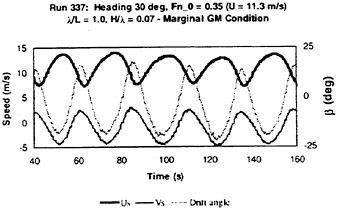
Figure 29. Ship velocities and drift angle associated with run 337
CONCLUSIONS
An extensive series of model tests with an intact frigate-type hull form were carried out to obtain data on extreme motions and capsizing in critical wave conditions. To control the conditions leading to these events, all tests comprised regular waves of moderate to extreme steepness. Through these tests and some numerical simulations the paper discusses physics associated with the following extreme motion events in astern wave conditions:
-
Periodic surging and surfriding
-
Broaching
-
Extreme rolling
-
Capsizing
Tests leading to surfriding show that a ship could attain transient speeds that exceed not only the calm water speed, but also the wave phase speed; bow submergence causes a significant increase in resistance and subsequent deceleration. Numerical simulations show a similar behavior, albeit with less excessive speed variations. Also, the numerical model, which makes use of linear wave theory, underpredicts wave celerity and hence surfriding speeds for steep wave conditions.
The hull, which was directionally stable, did experience some broaching events; two modes of broaching were distinguished: (1) broach preceded by surfriding with steadily increasing heading deviation, and (2) large amplitude, low-frequency yaw oscillations.
KG was varied to simulate three load conditions in the model tests: (1) typical Full Load condition, (2) Marginal GM condition that just meets the navy stability criteria, and (3) a Failed GM condition. No capsizes occurred for the first two load conditions. The most extreme rolling (without capsizing) occurred at high speed (Fn≥0.3) in stern quartering
waves and was typically very asymmetrical. Large variations in forward speed contribute to asymmetric rolling, as the ship spends more time (at higher speed and with reduced transverse stability) in a wave crest than in the wave trough.
Three modes of capsize were distinguished for the Failed GM condition: (1) loss of transverse stability in the wave crest, (2) dynamic loss of stability associated with surge-roll-yaw coupling, and (3) broaching. Roll resonance conditions in beam or stern quartering waves did not lead to capsizing. The influence of ship speed is crucial: capsizing occurred only at (calm water) Froude numbers Fn≥0.30. The most critical heading conditions in terms of capsize were following to stern quartering waves (0 ° 45 degrees heading angle).
The model tests show that a ship in stern quartering waves of moderate to extreme steepness is subjected also to large variations in transverse drift velocities: drift angle fluctuations can have an amplitude of the order of 20 degrees. In addition, the ship can experience a significant mean (transverse) drift speed to leeward.
The intention of this paper is to shed some more light on the physics of ship motions in extreme conditions. Further analysis and validation of the numerical simulation model will take place as part of the Cooperative Research Navies project on Dynamic Stability.
ACKNOWLEDGEMENTS
The authors would like to express their gratitude to the Cooperative Research Navies Dynamic Stability group (navies from Australia, Canada, Netherlands, United Kingdom and United States, U.S. Coast Guard and MARIN) for their permission to publish this paper. Within the United States this work was sponsored by the Office of Naval Research (ONR 334) and the U.S. Coast Guard Engineering Logistics Center, Code 023.
REFERENCES
1. De Kat, J.O., “Irregular Waves and Their Influence on Extreme Ship Motions”, Proceedings 20th Symposium on Naval Hydrodynamics, Santa Barbara, August 1994, pp. 39–58
2. NAVSEA Design Data Sheet 079–1. Department of the Navy, Naval Ship Engineering Center. June 1976
3. Grim, O., “Das Schiff in von achtern auflaufender See”, Jahrbuch der Schiffbautechnischen Gesellschaft, Vol 45, 1951, pp. 264–289 (in German)
4. Kan, M., “Surging of Large Amplitude and Surf-riding of Ships in Following Seas”, J.S.N.A. Japan, Vol. 166, Dec. 1989, pp. 49–62
5. Fenton, J.D., “A fifth-order Stokes theory for steady waves”, Journal of Waterway, Port, Coastal and Ocean Engineering, ASCE, Vol. 111, 1985, pp. 216–234
6. Hamamoto, M., Enomoto, T., Sera, W., Panjaitan, J.P., Ito, H., Takaishi, Y., Kan, M., Haraguchi, T. and Fujiwara, T., “Model Experiments of Ship Capsize in Astern Seas—Second Report”, Spring 1997 Meeting J.S.N.A., 1997
NOMENCLATURE
|
Β |
Beam |
|
COG |
Center of gravity |
|
Fn |
Froude number |
|
Fn_0 |
Froude number in calm water |
|
GMT |
Transverse Metacentric Height |
|
GZ |
Transverse Righting Arm |
|
Η |
crest-to-trough wave height |
|
KG |
Height of the Center of Gravity above the Keel |
|
L or LPP |
Length between Perpendiculars |
|
LCG |
Longitudinal Center of Gravity |
|
T |
Wave period |
|
U or Us |
Forward ship speed (along x-axis of yawed reference frame with vertical z-axis) |
|
V or Vs |
Transverse ship speed (along y-axis of yawed reference frame with vertical z-axis) |
|
|
Roll Period |
|
β |
Drift angle (=arctan Vs/Us) |
|
Δ |
Displacement |
|
λ |
Wavelength based on linear theory (=gT2/2π) |
|
ρ |
Density of water |
DISCUSSION
A.Graham
Department of National Defence, Canada
Lt Cdr Tony Graham, a member of the UK Royal Corps of Naval Constructors on exchange in Canada, and it is in that capacity that I speak today. I would like to congratulate the authors for this well presented paper, and CR NAV for a very successful R&D project of which this paper represents only a small glimpse.
The model tests excluded the wind effects present in the Sarchin and Goldberg criteria presented in the paper. How important is the wind contribution to the capsize phenomenon?
I am currently engaged in a project with Dr. Kevin McTaggart (Defence Research Establishment Atlantic, Canada) in converting this CR NAV body of data and tools into a design code. I wondered how the authors foresee the development of a dynamic stability design code?
AUTHOR’S REPLY
We would like to thank Mr. Graham for his kind words.
Wind can certainly influence capsizing. The reasons we did not include wind in the tests are as follows.
-
An important objective of the tests is to provide validation material under known conditions; the presence of wind in the model basin would introduce unknown parameters, due to, e.g., limited and non-uniform wind field in the basin.
-
Simulations suggest that for following to stern quartering waves, wind (parallel to the wave direction) does not play a major role in broaching or capsizing.
For a ship (intact or damaged) at zero or low speed in beam sea conditions, wind may be very important. These conditions were not considered.
There are two possibilities for incorporating ship dynamics into a new design code:
-
Deterministic
-
Probabilistic (risk based)
In earlier CRNAV work we found that the current (deterministic) navy criteria could be supplemented by additional guidelines to safeguard a ship against wave-induced capsizing in a rational manner. These proposed guidelines consist of requirements related to the angle of vanishing stability and total area underneath the GZ curve as a function of hull form (vertical prismatic coefficient).
In the long term, a risk-based approach seems to be appropriate, as capsizing is not a deterministic phenomenon. Useful work is underway in this area.
DISCUSSION
J.Dalzell
Naval Surface Warfare Center, Carderock Division, USA
I had the impression from the title that there would be more results presented from the simulation than turned out to be the case. The paper is clearly a summary of a monumental amount of work, still in progress, on a difficult subject. Therefore, I forgive the authors for not instantly gratifying my wishes for a lot of comparisons of simulation and experiment. Apart from one complaint, these remarks will be mostly in support of extracting information the authors may not yet be prepared to give.
The complaint is that the line conventions for all the time-history plots with more than two traces are nearly unintelligible for old eyes. With the authors’ physical explanation, the higher than phase speed transient surf riding speeds are not so difficult to understand. What are the prospects for including the gravitational acceleration and the augmented resistance into the simulation—or was this already there?
The comparisons of simulation and experiment in Figs. 10 and 11 do have some similarity at the end, but I would say that the beginning of the records represent quite different initial conditions. Can arbitrary initial phasing with the waves be simulated—or do the comparisons given already reflect a simulation of the experimental initial conditions?
In this connection, how was the nominal speed determined? Was the model accelerated to speed by self propulsion or some artificial means?
The text suggests that an earlier version of the simulation was run in order to help design the test matrix and its parameters. Now that the tests are run, can you tell us if there were any surprises—things that were not anticipated by the then version of the program.
AUTHORS’ REPLY
We would like to thank Mr. Dalzell for his comments. Our original intention was indeed to present many comparisons between measured and predicted events, such as capsizing. Comparisons between the tests and numerical predictions are still ongoing, however, in the following order:
-
Hydrostatics (GZ curves)
-
Roll decay tests in calm water at zero and forward speed
-
Calm water maneuvering (zigzag tests)
-
Seakeeping tests (non-capsize conditions)
-
Broaching and capsize tests
The critical remark on the line conventions used in the time series plots is certainly justified; we are looking for alternative ways to present such results in the future (the original curves were in color).
As regards predicting surf riding, the simulation model does include the effect of gravitation (all forces, including the gravitational force, are transformed to the rotated ship-fixed coordinate system before solving the equations of motion at each time step). We use a rather heuristic approach for estimating ship resistance at each time step: it is given by the calm water resistance associated with the instantaneous ship speed, corrected for the change in mean draft at the center of gravity of the ship. Obviously this does not provide a complete description of the time-dependent resistance force acting on the ship in large amplitude, following seas, but it does contain some of the critical elements needed to predict surf riding.
The nominal ship speed is the speed that the ship would attain at a given propeller RPM in calm water. To conduct a test at a certain nominal speed in waves, the propeller RPM would be set at the corresponding RPM level obtained from calm water performance tests. At the beginning of a test run in waves, the model was first held stationary with respect to the carriage, until a sufficient number of waves had passed the model. Subsequently the model would start to accelerate under its own power at a low RPM setting; after a few wave encounters, the RPM was set to the nominal speed level and the ship would attain its intended speed. This start-up process makes it very hard to reproduce in a simulation a test from the very beginning exactly.
In principle, the simulation can be started at arbitrary phasing with respect to the wave, and with any initial position and velocity for the six degrees of freedom. This must be done however, for a known and fixed propeller RPM setting. The intention is to compare selected test runs in the time domain as of a point in time where the nominal RPM setting has been reached. For this purpose, it is necessary to have exact information on where the wave is in relation to the model; these data are still being extracted from the test results:
As to the question on “surprises,” even though we have not been able to make detailed capsize comparisons yet, we have come across some unexpected results, some of which are the following:
-
Even in the severest test conditions, the ship did not capsize at all in the “Marginal GM” loading condition, while according to the predictions some capsizes should have occurred. In case of observed capsizes in the “Failed GM” condition, the simulation model predicts capsize events also. In general the predictions seem somewhat conservative (i.e., simulated capsizing occurs earlier than in the physical case).
-
The ship broached less than expected.
-
The speed fluctuations in surge and sway directions in steep, stern quartering sea conditions were larger than anticipated.
-
Sideways drift was more significant than anticipated in steep stern quartering waves.
Capsize Analysis for Ships with Water Shipping On and Off the Deck
J.Huang,1 L.Cong,1 S.Grochowalski,2 C.-C.Hsiung1 (1DalTech, Dalhousie University, Canada, 2Consultant, Canada)
Abstract
A prediction method of water shipping on and off the deck was developed and the computed results were validated by model tests. The amount of water trapped on the deck varies with time. The shallow water wave equations are solved to obtain the force caused by water flow on deck. The nonlinear equations of ship motion were solved in the time domain to study the capsize of vessels with the varying mass of water flow on deck.
Introduction
The effect of water flow on deck on ship motions, especially for small vessels, is very significant from the view point of safe operations in waves (Caglayan and Storch, 1982; Grochowalski, 1989, Huang and Hsiung, 1996a). For small fishing vessels, the heeling moment caused by water flow on deck can be of the same magnitude as the righting moment. Most of earlier research work was based on a simplified model of water flow on deck in which the free water was assumed to be frozen and the exciting forces were computed from the static weight. Studies of the dynamic effect of water flow on deck on the ship motion were rather scarce.
A prediction method for the mass of water shipping on deck was developed by Grochowalski (1979). The model was based on a horizontal relative velocity between the water particle and the bulwark for a ship in regular beam waves. An analytical expression representing the mass of water shipping on the deck during one wave period was determined. It was then extended to cover motions in oblique waves, and further improved by incorporation of the wave deformation due to the ship presence. In addition, velocities induced by the difference in heights between the wave surface and the bulwark edge were included by using a hydraulic model (Goda 1978, Grochowalski 1981).
Numerical analysis of the shallow-water flow on deck and the resulting force on deck has been carried out by some researchers. Dillingham (1981) used the Random Choice method for the computation of nonlinear shallow water flow on a two-dimensional deck. Pantazopoulos (1988) applied this method to a three-dimensional deck space. Huang and Hsiung (1996b) introduced the Flux-Difference Splitting method to compute the shallow water flow on deck. A flux limiter has been devised for this second-order finite difference scheme. This scheme gives satisfactory results without non-physical spurious oscillations. Based on this approach, the effect of water flow on deck on the motions of fishing vessels was investigated by Huang and Hsiung (1996a).
Adee and Pantazopoulos (1986) published their experimental work on motion responses of a two dimensional ship section in waves with water on deck. The roll motion appeared irregular in regular waves due to the water flow on deck. With a high metacentric height and a small amount of water on deck (about 10% of the model displacement), the roll motion might be reduced by sloshing of the trapped water. If the metacentric height was low and/or a large amount of water was trapped on deck (about 25% of the model’s displacement) the roll motion was enlarged. Capsize was observed in several situations. Lee and Adee (1994) computed sway, roll and heave motions of a long cylinder including the free water on
deck. The forces resulted from the water flow on deck were obtained from the 2-D Random Choice method given by Dillingham (1981).
Recently, Vassalos et al. (1997) studied the RO-RO ferry capsize due to flood water on the vehicle deck. Water inflow and outflow were modeled by the hydraulic approach. A correction factor was applied based on the results of experiment. The forces caused by water on deck were computed assuming that the water surface was a horizontal plane.
In this work, the time-domain ship motion was solved with considering water flow on deck. In fact, the water is coming on the deck due to large amplitude motions and large waves, meanwhile the water also escapes off the deck. The amount of water on deck varies with time. The prediction method of water shipping on and off the deck was developed. It combines numerical computation, hydraulic model and corrections based on physical model test data. Physical model tests for water shipping on and off the deck, and water sloshing on deck were conducted by the authors for validation of numerical computations. Results of the validation are presented in this paper.
In the ship motion analysis, the Froude-Krylov force and restoring force were calculated based on the instantaneous wetted hull surface under the incident wave profile whereas linear radiated and diffracted wave forces were employed, as de Kat and Paulling (1989) and Magee (1994). Maneuvering forces, rudder forces and the nonlinear roll damping were also included in the equations of ship motion. A computer program was developed based on the method described in this paper. It was applied to simulate a fishing vessel capsize with green water on deck.
Methodology
The Coordinate Systems
Three coordinate systems are employed for the ship motion analysis as shown in Fig. 1. OXYZ is the space-fixed coordinate system with the OXY plane on the calm water surface and the OZ axis is positive upwards. The second coordinate system om xm ym zm is a moving system which moves with the same steady forward speed as the ship in the OX direction. The om xm ym plane always coincides with the OXY plane, the om xm axis is in the same direction as the OX axis and the om zm axis is positive upwards. The third coordinate system os xs ys zs is fixed on the ship with the os xs ys plane coincident with the OXY plane when the ship is at its static equilibrium position, and the os zs axis is positive upwards.
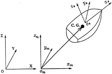
Fig. 1 Coordinate systems for ship motions
Equations of Ship Motion
The oscillatory ship motions are described in the om xm ym zm system. The ship motions are represented by (ξ1, ξ2, ξ3, e1, e2, e3), in which, (ξ1, ξ2, ξ3) are the displacements of the centre of gravity, and (e1, e2, e3) are the Eulerian angles of the ship in space. The Eulerian angles are the measurements of the ship’s rotation about the axes which pass through the centre of gravity of the ship. The instantaneous translational velocities of ship motion in the directions of os xs, os ys and os zs are u1, u2 and u3, respectively, and the rotational velocities about axes parallel to os xs, os ys and os zs and passing through the centre of gravity are u4, u5 and u6, respectively. The equations of ship motion are:
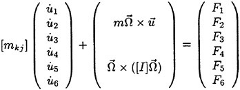
(1)
where ![]() is the generalized mass matrix:
is the generalized mass matrix:
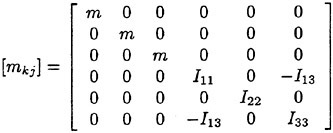
(2)
and [I] is the moment of inertia matrix
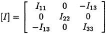
(3)
in which m is the mass of the ship, Ikk (k=1, 2, 3) denote the moments of inertia of the ship, and Ikj (k≠j) are the products of inertia of the ship. The total external forces on the ship are
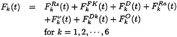
(4)
where ![]() are the restoring forces;
are the restoring forces; ![]() are nonlinear Froude-Krylov forces;
are nonlinear Froude-Krylov forces; ![]() the diffracted wave forces;
the diffracted wave forces; ![]() the radiated wave forces;
the radiated wave forces; ![]() the viscous damping forces;
the viscous damping forces; ![]() the nonlinear forces due to water flow on deck; and the force component
the nonlinear forces due to water flow on deck; and the force component ![]() may include the hydrodynamic maneuvering forces, the rudder force, propeller thrust, viscous resistance and cross-flow drag.
may include the hydrodynamic maneuvering forces, the rudder force, propeller thrust, viscous resistance and cross-flow drag.
The ship translational displacements (ξ1, ξ2, ξ3)T in the steady moving system and the Eulerian angles (e1, e2, e3)T are solved from:
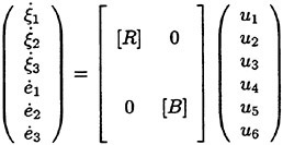
(5)
where matrices [B] and [R] are defined as follows:
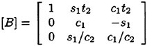
(6)
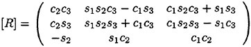
(7)
and ci=cos ei, si=sin ei, and ti=tan ei for i=1, 2, 3.
The Froude-Krylov forces, radiated wave forces and diffracted wave forces, rudder force, maneuvering forces, viscous forces have been discussed in the last ONR symposium (Huang and Hsiung, 1996a). In the next section, the effect of water flow on deck, water shipping on and off the deck, and the variable mass of water trapped on deck are studied.
Forces on the Deck
Normally, the effect of water on deck on the ship’s roll motion was studied by assuming that the amount of water on deck was known and it was a constant during the ship motion (Huang and Hsiung, 1997). In reality, the water is getting on and off the deck. Therefore, the mass of water trapped on deck varies with time. At a time instant, t, as the water depth and the water particle velocity are computed, the pressure on deck due to water flow can be obtained as follows:
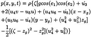
(8)
where (u, v)=velocities of water flow on deck.
As the roll angle increases, water cannot be trapped on the deck, and one side of the deck may deeply submerge into the wave. In this situation, the force on deck is resulted from the scattered wave field on the deck surface, and is different from that of water sloshing on deck. If there is a large motion of the submerged part of the deck relative to surrounding water, additional hydrodynamic pressure on the deck is generated (Grochowalski, 1989). Mathematical model of the forces on the submerged part of the deck is being under development and it will be published later. At the current stage, the pressure on the submerged deck surface is computed using the incident wave potential only, as for the rest of the immersed part of the hull:
(9)
where ζ-z is the wave elevation above the wetted deck and ![]() is the incident wave potential.
is the incident wave potential.
Therefore, by integrating the pressure, equation (8) or (9), over the deck area, we are able to obtain the forces and moments on deck due to the
deck water flow or the wave action on deck, respectively. Water can be trapped on deck at relatively small angles. The heeling moment caused by the deck flow can induce a large roll angle. When the deck is deeply immersed, or the roll angle is large, water will not stay on the deck, then the wave force instead of the water sloshing force acts on the ship. Therefore, a numerical switch has to be devised in the computer program to turn ON or OFF the deck flow force or the wave force on the deck accordingly to avoid an overlap of these two forces. We found that this switch was very important to the capsize simulation. At the current stage, it is designated in such a way that the “deck-in-water” mode is turned ON, while the “deck-flow” mode is turned OFF, when 30% of the deck area is submerged and the roll angle is greater than 23°.
Water flow on deck
Ship motions of six degrees of freedom have been considered in the numerical computation of the deck flow. The coordinate system oxyz for water flow on the three dimensional deck is shown in Fig. 2. It is fixed on the deck space with the oxy plane on the deck surface. The oz axis is positive upward and the origin ο is at the centre of the deck surface.
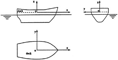
Fig. 2 Coordinate system for deck flow
The continuity equation and Euler’s equations of motion can be written as follows:
(10)
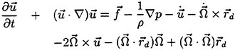
(11)
where ![]() u, v and w are velocity components of the water particles in x-, y- and z- directions, respectively; p is the pressure; and
u, v and w are velocity components of the water particles in x-, y- and z- directions, respectively; p is the pressure; and
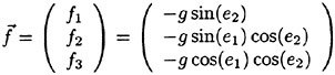
(12)
with ![]() and (xg, yg, zg) is the coordinate of the centre of gravity of the ship in the oxyz system.
and (xg, yg, zg) is the coordinate of the centre of gravity of the ship in the oxyz system.
Under the assumption of shallow-water depth, the governing equations (10) and (11) for the deck flow were simplified to the shallow-water equations in a non-inertial system. The Flux-Difference Splitting method was used in the numerical computation. The numerical method has been extensively validated against the published test data of water sloshing due to the deck’s roll motion. (Huang, 1995, Huang and Hsiung, 1996b).
For a swaying tank, a validation example of water sloshing time history is given in Fig. 3. The tank is 0.4 m wide with a mean water depth of 2.0 cm. The sway amplitude is 0.5 cm and the frequency is 3.471 rad/sec. The test data are taken from Iwamoto’s (1991) work.
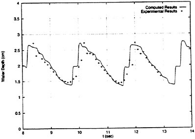
Fig. 3 Time history of wave motion due to sway, ω=3.471 rad/s, sway amp.=0.5 cm
Model tests for water sloshing on deck were conducted at CMVDR, Dalhousie University (Huang et al., 1997). The experimental setup is shown in Fig. 4. The tank size was 0.35m×0.35m×0.06m. The tank was forced to roll. Both wave motions and heeling moments were measured during the test.
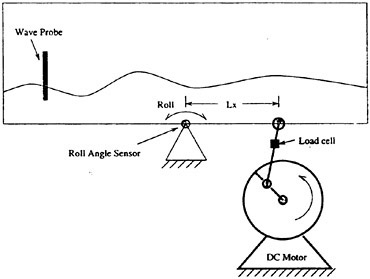
Fig. 4 Experimental setup for sloshing and water escaping of the deck
For the roll amplitude 3 deg, the roll frequency 3.769 rad/sec, and a constant volume of water with the mean water depth 3.2 cm, the time histories of the computed and measured wave motions are shown in Fig. 5. The time histories of sloshing moment, corresponding to the roll amplitude 5 deg, the roll frequency 3.41 rad/sec, and the mean water depth 2.5 cm, are shown in Fig. 6.
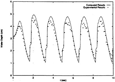
Fig. 5 Wave motion due to roll, ω=3.796 rad/s, roll amp.=3 deg
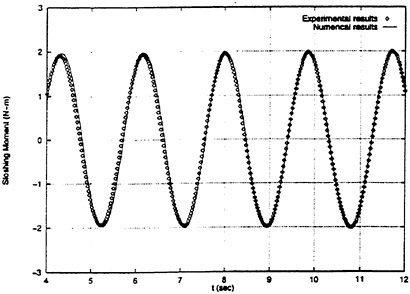
Fig. 6 Sloshing moment, ω=3.41 rad/sec, roll amp.=5 deg
The test results of sloshing moment by Van Der Bosch & Vugts (1966) were also used for the validation. The model tank used in the test was 1 m wide, the mean water depth was 6 cm, and the corresponding primary resonant frequency of sloshing in the tank was ω0=2.41 rad/sec. The amplitude of sloshing moment is shown in Fig. 7 and the phase lag in Fig. 8. The maximum moment is around ω0, and ![]() . At low frequencies, the phase lag is close to zero and at the high frequency end, the phase lag is approaching 180 degrees.
. At low frequencies, the phase lag is close to zero and at the high frequency end, the phase lag is approaching 180 degrees.
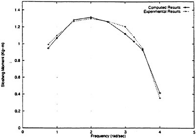
Fig. 7 Amplitude of sloshing moment, roll amp.=5.73 deg
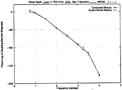
Fig. 8 Phase lag of sloshing moment, roll amp.=5.73 deg
The above comparisons show that a very good agreement has been achieved between the numerical computations and the physical model tests.
Water shipping on deck
With the ship’s presence in waves, the water surface around the ship hull is deformed. The actual wave elevation around the hull affects the water shipping on deck. In this work, the scattered wave elevation was calculated in the frequency domain and then converted to the time-domain computation. The 3-D panel method, which is based on the Green function method, is used in computing the velocity potential and its partial derivatives (Hsiung and Huang, 1991).
Four elements are considered in the computation of water shipping on deck, i.e, the hydraulic head of wave elevation, the water particle orbital motion in the incident wave, the diffracted and radiated wave field, and the ship motions.
A situation when the wave surface exceeds the bulwark edge is illustrated in Fig. 9, where Ζη is the vertical coordinate of the wave surface, Zi is the vertical coordinate of water surface inside the deck well, and Zfb is the vertical coordinate of the bulwark. The general condition for water shipping on deck is
(13)
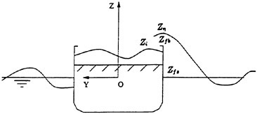
Fig. 9 Definition of wave surface position
When Ζη>Zi, the water surface outside the ship is higher than that in the deck well, hence water enters the deck well. By the law of energy conservation, the velocity due to the hydraulic head can be obtained by:
(14)
This is analogous to the flow over a weir. The corresponding rate of water per unit width in terms of time entering the deck well is:
(15)
The rate of water shipping onto the deck due to the orbital motion of water particles in the incident wave field is:
(16)
where k is the wave number, and u0(t) is the horizontal velocity of the water particles in the incident wave field on the free surface.
The rate of water shipping onto the deck due to the relative normal velocity of the ship motion is:
(17)
where us(t) is the normal velocity of a point on the bulwark with respect to the surrounding water. In the above equations, zb(t) is determined by
(18)
The total quantity of water shipping onto the deck is the superposition of the above three components. The viscous effect and other neglected effects are taken into account by introducing a correction factor, C0, to the formula of water shipping on deck as follows:
(19)
where the coefficient C0=0.55 was determined by fitting the model test data with the numerical results.
Finally, the volume of water shipping onto the deck as the function of time is calculated by:
(20)
where s is the contour of the bulwark.
The model test results (Grochowalski, 1996) of water shipping on deck were used to validate the computational method. The experimental setup is shown in Fig. 10. The cylindrical model was 1.8 m long and the radius was 0.425 m. The model was not allowed to oscillate during the test.
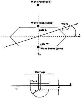
Fig. 10 Experimental setup for water shipping on deck
In these model tests, the control parameters were: wave height, wave frequency, heading angle, and model draft. Each test run lasted for a few wave periods. The wave elevation, the amount of water shipping on deck, and the number of periods for data recording were measured. Examples of the computed and measured wave elevations at the midship on the weather side of the model are shown in Figs. 11 and 12, for wave headings of 0 deg (following sea) and 90 deg, respectively.
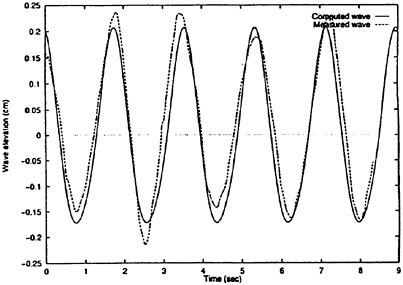
Fig. 11 Wave elevation amidships, β=0 deg
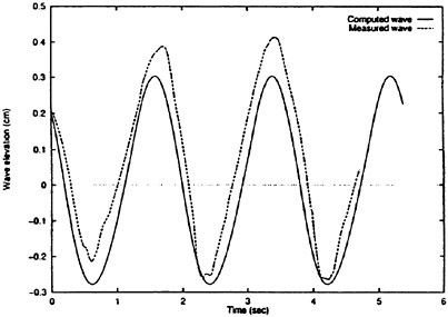
Fig. 12 Wave elevation amidships, β=90 deg
The test data of the mass of water shipping on deck for the wave amplitude 0.19 m, the wave period 1.8 sec and the draft 0.525 m were used here for validation. The wave heading in the tests ranged from 0 deg to 90 deg as shown in Table 1. The computed mass of water shipping on deck and the test results are shown Fig. 13. Generally speaking, the agreement between test and compu-
tation is satisfactory.
Table 1. Parameters for water shipping on deck model tests
|
Test No. |
Wave Heading (deg) |
The Number of Periods of Recording |
|
1 |
0 |
6 |
|
2 |
0 |
5 |
|
3 |
15 |
5 |
|
4 |
30 |
4 |
|
5 |
45 |
3 |
|
6 |
90 |
3 |
|
Wave Amplitude=0.19 m Wave Period=1.8 sec. Model Draft=0.525 m |
||
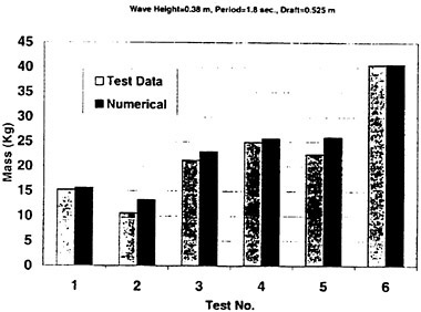
Fig. 13 Mass of water shipping on deck
Water escaping off the deck
An experiment has been carried out to understand the physical phenomenon and to validate the numerical model of water escaping off the deck. The same experiment setup was used as for sloshing experiments (Fig. 4). During the experiment, the water depth and the amount of water spilling out of the deck over bulwark were measured. The tank was forced to roll. The oscillation frequency ranged from 0.5ω0 to 2ω0, where ω0 is the resonant frequency of sloshing in the tank. Each test run lasted for four periods of time of the deck oscillation, except for the cases of roll amplitude 15 deg in which the test only lasted for one period of time.
Two modes of water escaping from the tank (deck) were observed in the test. One was like a “waterfall” (Fig. 14), and the other was like a “splash” (Fig. 15).
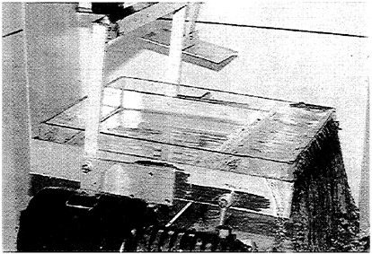
Fig. 14 Water escaping off the deck as the “waterfall” mode.
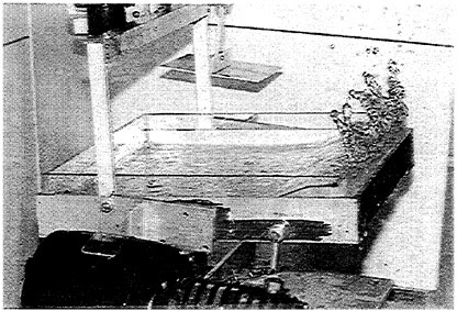
Fig. 15 Water escaping off the deck as the “splash” mode.
There was much more water escaping of the deck in the “water fall” mode than that in the “splash” mode. Hydraulic bore and progressive solitary waves were typical wave patterns observed in the experiment. Water escaping off the deck depends on the water depth at the deck edge, bulwark height, deck motions and the phase difference between the deck motion and the sloshing motion.
Based on the experimental observation and water flow over a weir and a slope as given by hy-
draulics textbooks (Hwang, 1981), the following formulas are developed for water escaping off the deck. The amount of water escaping off the deck over bulwark as the function of time is:
(21)
where the correction coefficient C=2.5, s is the contour of the bulwark, and he is the height of escaping water over the bulwark:

(22)
in which hi is the vertical coordinate of water surface inside the deck, ho is the vertical coordinate of water surface outside the deck, and hb is the vertical coordinate of the bulwark, all the coordinates are in the space fixed coordinate system. Based on correlation analysis of the results from computation and experiments, we are able to produce the following semi-empirical formulas for the escaping velocity. At the starboard side,
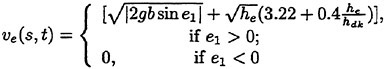
(23)
At the port side
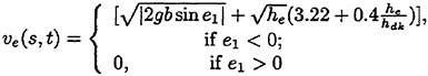
(24)
At the stern
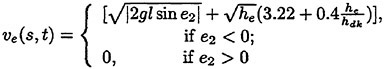
(25)
where b is the deck width, l the deck length, and hdk the depth of the deck well. The numerical method for the nonlinear shallow-water flow on deck was used to compute the wave motion inside the deck. Based on the above formulas, the amount of water escaping off the deck was computed at each time step. Then, for the next time step, the water depth was adjusted by subtracting a layer of water to account for the mass change due to water escaping off the deck.
Validation of the above numerical model has been carried out with the experimental data. Fig. 16 shows the computed and test results of water depth at the location close to the deck edge. The roll amplitude of the deck was 5 deg and the frequency was 6.28 rad/sec. The initial mean water depth was 3.2 cm. It can be seen that the water depth was decreasing since the water keeps escaping off the deck. After four cycles of the deck oscillation, the mean water depth was reduced to 2.4 cm.
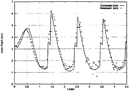
Fig. 16 Water depth on deck (with water escaping off the deck)
The computed mass of water escaping of the deck and the measured results are given in Fig. 17 for the initial mean water depth 3.2 cm, and the deck motion frequency 5.03 rad/sec. Fig. 18 shows the results for the initial mean water depth 2.6 cm, and the deck motion frequency 4.52 rad/sec. It can be seen that good agreement has been reached.
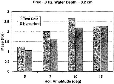
Fig. 17 Mass of water escaping off the deck, ω=5.03 rad/sec, d=3.2 cm
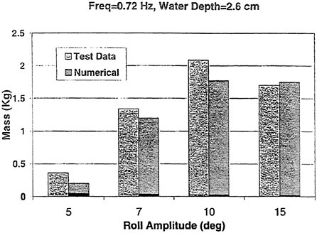
Fig. 18 Mass of water escaping off the deck, ω=4.52 rad/sec, d=2.6 cm
Capsize Simulation
The validation of the mathematical model developed and application of this study to analysis of ship stability safety in severe seas is being carried out by the authors. In this paper, some simulation results of ship motions with water sloshing on deck while the amount of water is changing during the motion are presented. The simulations were performed for a fishing vessel. The main dimensions of the vessel are given in Table 2.
Table. 2 Characteristics of the fishing vessel
|
Length overall, Loa (m) |
19.78 |
|
Beam, B (m) |
6.09 |
|
Depth, D (m) |
3.68 |
|
Draft at FP (m) |
2.98 |
|
Draft at AP (m) |
2.59 |
|
Displacement (m**3) |
145.7 |
|
Metacentric Height GM (m) |
0.49 |
|
Roll period (sec) |
6.51 |
The longitudinal half-body of the panelized hull including the deck, deck house and bulwark is shown in Fig. 19.
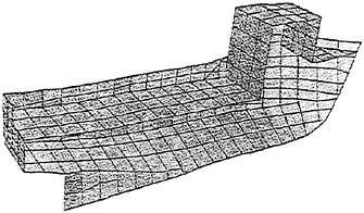
Fig. 19 Panelized hull used in the simulation
Regular waves of the steepness (2ζa/λ) about 0.12 were used in the simulation. The steep waves were modeled by the 2nd-order Stokes waves. Fig. 20 shows the motion simulation and the respective amount of water trapped on the deck. The wave conditions were: wave height 2.975 m, wave frequency 1.527 rad/sec and wave heading 30 deg. The Froude number was 0.287.
At the time about 30 sec, water started to ship on deck as a result of large roll and heave. Near t=40 sec, a large amount of water was trapped on deck, and the roll and heave motions reached their maximum values. From t=50 sec to 88 sec, the amount of water was kept constant due to moderate heave and roll motions. The heave and pitch motions appeared to be quite regular. There were a sinkage and trim in heave and pitch due to the water on deck. It seems that the heave and pitch motions were not as sensitive to the change of the water mass on deck as the roll motion was.
It should be pointed out that the amount of water on deck might be overpredicted since freeing ports were not modeled in the analysis of water shipping on and off the deck.
To illustrate the influence of water on deck on the ship behavior in a more dramatic situation, a simulation was carried out in a larger wave. The wave conditions were: wave height 4.402 m, wave frequency 1.292 rad/sec and wave heading 90 deg. The Froude number was 0.273. The roll, heave, pitch motions and the respective amount of water on deck are shown in Fig. 21. The vessel capsized in a very short period of time (less than 7 seconds) due to a large amount of water shipping on deck which caused large amplitude rolling and deep deck immersion in water.
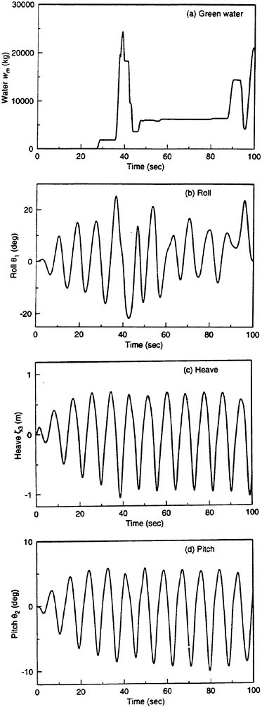
Fig. 20 Green water and respective motions (hw=2.975 m, ω=1.527 rad/sec, β=30° and Fn=0.287).
It is interesting to observe, from Fig. 21, the sequence of the ship motion relative to the amount of water shipping on and off the deck. The heave motion was quite regular and oscillating about the mean sinkage position. The pitch motion shows a strong correlation between the water mass on deck. When large amount of water is accumulated on the deck (46 sec to 55 sec) the ship was pitching with smaller amplitudes with respect to a trim by the stern where the most of water was accumulated. As water was shed off the deck, the pitch motion was more symmetric and with larger amplitudes. Near t=40 sec, the ship had a large roll angle at which the deck was immersed in the wave. Water may not stay on deck with only a very small amount of water trapped as shown in Fig. 21(a). From t=46 sec to 55 sec, a large amount of water was trapped on the deck. The trapped water caused a large roll angle (40 deg). When the water was shed off the deck, the roll decreased (at t=58 sec). When water shipped on deck as result of the next two large roll amplitudes, the ship capsized at t=74 sec.
Conclusions
The mathematical model of ship motions with water flow on deck presented in this paper provides possibility to study ship behavior in extreme wave conditions when green water is shipping on and off the deck. The model includes a theoretical method for prediction of mass of water shipping on deck, a method for calculating the amount of water escaping off the deck and a mathematical model of water flow on deck. An essential characteristic of the model presented is that, as it is in the real situation, the amount of water flowing at the deck is varying with time as a result of waves action and ship motions.
Ship motions of 6-degrees of freedom are represented by equations in which nonlinear effects of the Froude-Krylov forces, deck flow forces, viscous damping and manoeuving forces are included. The linear radiation and diffraction forces are computed in the frequency domain, and then converted into the time domain. Steep and large waves are represented by periodic, 2nd-order Stokes waves. The equations of motion are solved in time domain.
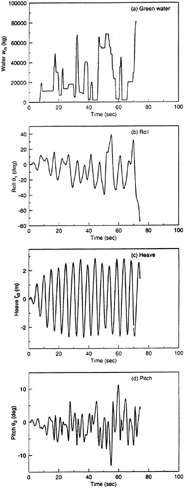
Fig. 21 Green water and respective motions hw=4.402 m, ω=1.292 rad/sec, β=90° and Fn=0.273).
The theoretical model for prediction of amount of water shipping on deck is based on relative velocity of water particles in the wave motion in combination with the mass flow due to the hydraulic head for the wave height over the bulwark. The model includes the wave deformation at the ship sides. Experimental results of water shipping on deck have been used for the validation. The predicted mass of water agrees reasonable well with the measured results.
Mathematical model of water escaping of the deck is based on hydraulic formulas for water flow over a weir and a slope. Semi-empirical formulas were established to compute the escaping velocity. An experiment for modeling water escaping off the deck was conducted under the forced roll excitation. Two patterns of water escaping off the deck in the form of “waterfall” and “splash” have been observed. Generally speaking, the maximum amount of water escaping off the deck occurs around the resonant frequency of sloshing in the deck well. Based on the test results, corrections have been made on the numerical model of water shipping on and off the deck.
A computer program based on this mathematical model was used for simulations of the behavior of a small vessel subjected to water shipping on and off the deck in large waves. The simulation results demonstrate a strong correlation between the varying mass of water on deck and the subsequent motions of the ship. Incorporation of the numerical scheme for continuous computing of the instantaneous mass of water on deck constitutes an essential improvement to the prediction methods of ship motions with water on deck and make the simulation results much closer to the reality. The results also show that water sloshing on deck, even if its mass is decreasing with the roll, may cause a capsize.
The theoretical model presented in this paper is still being validated against physical model tests of ship capsizing in large and steep waves. After the validation process is completed, the software can be used as a tool to evaluate stability safety of ships in extreme conditions.
Acknowledgments
The authors wish to express their gratitude to Transport Canada, Marine Safety, and Natural Sciences and Engineering Research Council of Canada for their support of this research.
References
Adee, Β.Η. and Caglayan, I., “The Effects of Free Water on Deck on the Motions and Stability of Vessels”, Proceedings of the Second International Conference on Stability of Ships and Ocean Vehicles, Tokyo, Japan, 1982.
Adee, B.H. and Pantazopoulos, M.S., “Experimental Investigation of a Vessel Response in Waves with Water Trapped on Deck”, Proceedings of the Third International Conference on Stability of Ships and Ocean Vehicles, Gdansk, Poland, 1986.
Caglayan, I. and Storch, R.L., “Stability of Fishing Vessels with Water on Deck: A Review”, Journal of Ship Research, Vol. 26, No. 2, June 1982.
de Kat, Jan O. and Paulling, J.R., “The Simulation of Ship Motions and Capsizing in Severe Seas,” Transactions, SNAME, Vol. 97, 1989.
Dillingham, J., “Motion Studies of a Vessel with Water on Deck”, Marine Technology, Vol. 18, No. 1, 1981.
Goda, K. “A Study of Shipping Water Pressure on Deck by Two-Dimensional Ship Model Test”. Journal of Society of Naval Architects of Japan, vol. 143, June 1978.
Grochowalski, S. “Calculation of the Amount of Water Shipping on Deck in Shallow Water Beam Waves” (in Polish and German). Report of Inst. Okr. PG (Tech University of Gdansk), No 1210/MR-324/79, Gdansk, 1979.
Grochowalski, S. “Theoretical Prediction of the Mass of Water Shipping on Deck in Irregular Waves”, (in Polish). Report of Inst. Okr. P.G. (Techn. Univ. of Gdansk) No. 1969/MR-514/81. Gdansk, 1981.
Grochowalski, S., “Investigation into the Physics of Ship Capsizing by Combined Captive and Free Running Tests”, Transactions, SNAME, 1989.
Grochowalski, S. “Model Tests of Water Shipping on Deck in Waves”, NRC/IMD Report, 1996.
Hsiung, C.C. and Huang, Z.J., “Comparison of the Strip Theory and the Panel Method in Computing Ship Motion with Forward Speed”, Proceedings of Symposium on Selected Topics of Marine Hydrodynamics, St. John’s, Nfld, 1991.
Huang, Z.J., Nonlinear Shallow Water Flow on Deck and Its Effect on Ship Motion, Ph. D. Thesis, Technical University of Nova Scotia, Halifax, Nova Scotia, 1995.
Huang, Z.J. and Hsiung, C.C., “Nonlinear Shallow Water Flow on Deck Coupled with Ship Motion”, Proceedings of the 21st Symposium on Naval Hydrodynamics, Trondheim, Norway, 1996a.
Huang, Z.J. and Hsiung, C.C., “Nonlinear Shallow-Water Flow on Deck”, Journal of ship research, Vol. 40, No. 4, 1996b
Huang, Z.J. and Hsiung, C.C., “Dynamic Simulation of Capsizing for Shallow Draft Vessels with Water on Deck”, STAB’97, Varna, Bulgaria, 1997.
Huang, Z., Cong, L., Hsiung, C.C., and Grochowalski, S., “Development of an Analytical Tool for Examination of Stability of Ships in Extreme Seas”, Technical Report CMVDR-97–01, Centre for Marine Vessel Design and Research, Faculty of Engineering, Dalhousie University, Halifax, Nova Scotia, 1997.
Hwang, N.H.C., Fundamentals of Hydraulic Engineering Systems, Prentice-Hall, Englewood Cliffs, 1981.
Iwamoto, S., “Numerical Analysis of Shallow Water Dynamics on Deck”, Journal of the society of Naval Architects of West Japan, Vol. 86, 1991.
Lee, K. and Adee, B., “Numerical Analysis of a Vessel’s Dynamic Responses with Water Trapped on Deck”, Proceedings of the Fifth International Conference on Stability of Ships and Ocean Vehicles, Melbourne, Florida, 1994.
Magee, A., “Seakeeping Applications Using a Time-Domain Method”, Proceedings of the Twentieth Symposium on Naval Hydrodynamics, Santa Barbra, California, August, 1994.
Pantazopoulos, M.S., “Three-dimensional Sloshing of Water on Deck”, Marine Technology, Vol. 25, 1988.
Vassalos, D., Turan, O. and Pawlowski, M., “Dynamic Stability Assessment of Damaged Passenger/Ro-Ro Ships and Proposal of Rational Survival Criteria”, Marine Technology, Vol. 34, No. 4, 1997.
Van der Bosch, J.J. and Vugts, J.H., “On Roll Damping by Free-Surface Tanks”, Transactions, RINA, Vol. 108, 1966.
DISCUSSION
J.de Kat
Maritime Research Institute, The Netherlands
The authors present an interesting simulation method that combines large amplitude motions integrated with the dynamics of water flow on deck. An important factor in the simulation process is the interaction between the hull and surrounding wave field, which affects the shipping of water. In this respect I would like to ask the authors the following:
-
Do the physics (experimental observations) of shipping water on deck justify the separation and linear superposition of velocity contributions, as given by Eq. (19)?
-
Presuming the parameter Ζη (t) represents the vertical coordinate of the disturbed wave surface, have the authors considered basing the wave orbital velocity at the hull on the combined incident, diffracted and radiated waves, instead of using Eq. (16)?
-
Could the authors comment on the possible importance of steady and dynamic swell-up effects, associated with the ship’s forward speed in waves, with respect to the relative wave elevation along the bulwark?
-
Could the authors elaborate on the procedures for estimating the correction factors C0 in Eq. (19) and C in Eq. (21), and on the conditions for which these factors apply (e.g., hull shape, ship speed, wave parameters, and heading angle)?
AUTHORS’ REPLY
In the model test of water shipping on deck, we had a total of 43 runs, which were subject to various loading conditions and wave conditions. The separation and linear superposition given in equation (19) can be justified when water enters the deck space over the bulwark. Results of comparison between the predicted and measured mass of water on deck from the 43 runs will be included in our paper “Theoretical Modeling of Ship Motions and Capsizing in Large and Steep Waves,” which will be presented at the SNAME Annual Meeting at San Diego this year. In the model test, we did not measure the velocity of the water particle over the bulwark.
The disturbed wave surface around the hull was computed from the linear diffraction theory. The relative normal velocity in the disturbed wave field above the bulwark cannot be calculated theoretically. Equation (16) was used to calculate the rate of water shipping on deck due to the orbital motion in the portion of incident wave over the bulwark.
The dynamic swell effects are important to the relative motion and the water shipping into the deck, especially for computing the hydraulic head as given in equation (14). The diffracted wave effect can be found from Figure 12. The incident wave amplitude is 0.19 m in the model test, while the maximum wave elevation along the bulwark can be 0.4 m. In computation, the steady Kevin wave due to the steady forward speed of the ship was not included.
The correction factors in equations (19) and (21) were determined by minimizing the RMS of the difference between the test data and the calculated results. The water shipping on the deck tests were conducted using a cylindrical model in steep regular waves with the wave heading from 0 to 90 degrees. The model had no forward speed; however, it had a transverse drift velocity. The formulae can be applied to ships on which the deckhouse is located close to the bow. This means that water mainly enters the deck space from the sides of the hull rather than over the bow.
Fully Nonlinear Free-Surface Computations for Arbitrary and Complex Hull Forms
A.Subramani, R.Beck (University of Michigan, USA)
S.Scorpio (Design Research Engineering, USA)
ABSTRACT
In this paper is described the successful extension to realistic hull forms of a desingularized boundary integral method that computes fully nonlinear, inviscid water waves in the time domain and which had been limited thus far to applications involving mathematical body shapes. Results are presented for the Series 60, CB=0.6 advancing in calm water for two different Froude numbers. The calculated wave profile and wave cuts are shown to be in good agreement with the experimental data.. The method is also successfully demonstrated for a ship with a bulbous bow as a prelude to the extension of the method for a naval combatant. Lastly, ways in which recent work on two-dimensional inviscid transom stern flow could be extended to compute the flow characteristics of three-dimensional transom sterns are discussed.
INTRODUCTION
Concomitant with the improvements in the techniques for the design of ships and offshore structures has been an increase in the demand for improved analysis tools. This is especially so in the area of marine hydrodynamics, as indicated by the degree to which the computational methods are being extended for use in the testing of newer naval combatant designs.
The very use of Numerical Hydrodynamics tools in the design process is aided considerably by the availability of many, diverse solution methodologies, each with its own different strengths and drawbacks. The wide choice in methodologies probably owes most to two factors: the essential difficulty of marine hydrodynamic computations and the relentless increases in computational power over the last few decades. The latter is recognized widely; to elaborate on the former: even the reduction to potential flow leaves significant challenges because of the nonlinear nature of the free surface boundary conditions and the complex geometric features of typical marine vehicles. This paper will discuss recent advances made with a particular potential flow solver—in particular, the solving of fully nonlinear hydrodynamic problems for arbitrary and complex hull forms.
Fully nonlinear potential flow computations can be performed in many ways. For steady forward speed problems, fully nonlinear computations may be performed by using an iterative technique to solve a series of linearized boundary value problems that are based on the solution to the previous iteration and which are satisfied on the deformed free surface and the exact wetted surface of the body. Iterative techniques have been used successfully by, among others, Jensen et al. (1), Kim and Lucas (2) (3), Raven (4), and, more recently, Scullen and Tuck (5), or Scullen (6). These techniques have the likely advantage of converging to the fully nonlinear solution in less computer time than a time-stepped method, but they cannot be extended easily to unsteady seakeeping problems.
A time-domain solution of the fully nonlinear water wave problem may be obtained using the Euler-Lagrange method, which was introduced by Longuet-Higgins and Cokelet (7) in their study of two-dimensional water wave problems. This time-stepping method consists of two major tasks at each time step: In the Lagrange phase, individual nodes on the free surface are tracked by integrating the nonlinear free surface conditions with respect to time, while in the Euler phase a mixed boundary value problem is solved to obtain the fluid velocities that in turn are needed in the integration of the free surface boundary conditions.
Variations of the Euler-Lagrange method have been applied to a wide variety of two- and three-
dimensional problems. However, the variations arise primarily from differences in the time-integration schemes used and in the techniques used to solve the resulting mixed boundary value problem at each time step. The vast majority of results have been obtained for applications limited to mathematical body geometries such as cylinders, spheroids, and the Wigley hull, or for water wave problems with no body at all.
At the University of Michigan, a multipole-accelerated desingularized boundary integral method—denominated UM-DELTA, for University of Michigan Desingularized Euler-Lagrange Time-Domain Approach—has been developed over the past several years to solve fully nonlinear water-wave problems including wave loads on offshore structures and nonlinear ship motions. The development of the UM-DELTA method was recently chronicled by Beck (8). As previously indicated, in this method the fluid is assumed incompressible, inviscid and started from rest so that the resultant flow is irrotational and governed by the Laplace equation for the velocity potential.
The velocity potential is constructed by singularities distributed on auxiliary surfaces separated from the problem boundaries (hence, ‘desingularized’) and outside the flow domain—‘above’ the free-surface and ‘inside’ the body surface, and ‘outside’ the appropriate boundaries at infinity. The strengths of the singularities are determined so that the boundary conditions are satisfied at chosen collocation points or nodes. [Figure 1. (a) provides a perspective view of the typical grid distribution on the body and the free surface, while in figure 1. (b) are sketched the relative locations, at a representative cross-section, of the nodes and the desingularized sources.] To ensure the convergence of the method, the desingularization distance decreases as the computational grid becomes finer. Because of the desingularization, the resulting kernel in the integral equation is nonsingular; therefore, special care is not required to evaluate integrals over the panels. Simple numerical quadratures can be used to reduce the computational effort greatly. Further, simple isolated Rankine sources may be used, allowing the direct computation of the induced velocities in the fluid without further numerical integration or differentiation. The solution is advanced in time using the Euler-Lagrange time-stepping procedure and the body position and surface normal velocities are updated from the equations of motion of the vessel.
As discussed in Scorpio et al. (9), multipole acceleration techniques have also been implemented within UM-DELTA. The underlying idea of multipole acceleration is that the potential due to a group of sources may be evaluated at distant points by first accumulating the influences into a single multipole expansion. By a complementary arrangement of the evaluation points into groups, the accumulated multipole expansions may be transformed into local expansions centered around each group. Using a tree-structured hierarchy of source groups and evaluation point groups, the normally O(N2) process of evaluating the influence of Ν sources at Ν points is reduced to an O(N) process with only an O(N) storage requirement. This leads to substantial reductions in computational time and storage, enabling the simulations to be performed on high-end workstations. However, because of the extensive requirements for logical branching, multipole acceleration disrupts the high degree of vectorization inherent in the UM-DELTA code and is not, therefore, invoked on vector supercomputers such as the CRAY C-90. On the other hand, it also allows for easier implementation of the method on scalable parallel computers and thus presents a useful option on more than one platform.
To date, the UM-DELTA method has been successfully applied to a wide variety of problems. These include: the generation of shallow water solitons [Cao et al. (10)]; wave resistance, added mass, and damping and exciting forces on a Wigley hull [Beck et al. (11)]; and wave loads on a vertical cylinder [Scorpio and Beck (12)]. However, the applications thus far have been limited to simplified body shapes—body shapes that could be represented mathematically.
An accurate and efficient modeling of the geometry is not a trivial task within UM-DELTA. Unlike panel methods that use flat quadrilateral panels to define the surface and the unit normal, UM-DELTA needs to be able to determine the surface location and unit normals at arbitrary node locations on the body. Determining the surface location and unit normal at arbitrary locations on a typical ship hull has been difficult, and it has served as a hurdle in the extension of the method to arbitrary hulls. Nevertheless, the first such extension was carried out by Celebi and Beck (13), who used a NURBS (Non-Uniform Rational B-Spline) surface representation of the body surface and a variational adaptive curve grid generation method for node placement on the body. However, the use of this technique:—when tested on the parabolic Wigley hull modified with the inclusion of bow and stern rakes—resulted in a 40% increase in CPU time when compared to a calculation that used instead the mathematical representation of the hull. Considering that the computational burden would only increase for ships with complex features such as bulbous bows and skegs, which may require more than a single NURBS surface to represent the hull
surface effectively, the NURBS technique was not pursued further.
Therefore, the development of a faster and more robust hull-surface processor was initiated and subsequently incorporated into the UM-DELTA code along with other improvements. This paper describes then the recent development of the method in its ongoing extension to arbitrary and complex hull forms, while also touching upon the inherent difficulties in the task.
In the following sections shall be presented a brief description of the geometry processor and a discussion of the recent efforts to handle wave breaking in the computations. Results of the calculations for arbitrary and complex hull shapes are then presented. Specifically, calm water results are presented for the Series 60, CB=0.6 hull, which typifies arbitrary body shapes, at two different Froude numbers. The calculations of the wave profile on the hull and wave cuts will be shown to compare well with experimental data.
The extension of the method for complex hulls such as naval combatants with bulbous bows and transom sterns was divided into two stages—seeking to render capable the handling of, first, bulbous bows and, then, transom sterns. The extensions for transom sterns have not been completed at the time of this writing. Therefore, the method is herein demonstrated for a ship with a bulbous bow alone (as far as complex geometric features are concerned). Additionally, the strategy to be adopted for handling the inviscid flow behind three-dimensional transom sterns is described by presenting some two-dimensional results. First, however, the theoretical background of the method is provided for the sake of completeness.
THEORETICAL BACKGROUND
Problem Formulation
Consider a vessel floating on a free surface and translating with speed Uo(t) in the negative x-direction with respect to a right-handed space-fixed coordinate system. For the (x,y,z) system attached to the body, the z=0 plane defines the calm water level, with +z directed upward and the x-z plane coincident with the centerplane of the vessel. The total velocity potential describing the fluid motion is then
(1)
where Uo(t)x is the potential due to the free-stream velocity and ![]() is the perturbation potential. In the fluid domain, both potentials Φ and
is the perturbation potential. In the fluid domain, both potentials Φ and ![]() satisfy Laplace’s equation,
satisfy Laplace’s equation,
(2)
In order to define a well-posed problem, boundary conditions must be specified on all surfaces surrounding the fluid domain. On the body wetted surface (SH) and on the bottom (SB), the boundary conditions are:
(3)
and
(4)
where ![]() is the unit normal out of the fluid and
is the unit normal out of the fluid and ![]() is the velocity of a point on the body due to unsteady ship motion and
is the velocity of a point on the body due to unsteady ship motion and ![]() is the velocity of the bottom relative to the 0(x,y,z) system. Because we are solving an initial value problem, the boundary condition on the surface at infinity (S∞) is
is the velocity of the bottom relative to the 0(x,y,z) system. Because we are solving an initial value problem, the boundary condition on the surface at infinity (S∞) is
(5)
Other far field boundary conditions are possible; for example, incident waves may be prescribed at the upstream boundary (SE). The boundary condition on an outer wall (Sw) aligned with the free-stream direction will have the form:
(6)
Downstream, an absorbing beach may be used; for forward speed problems, an open boundary condition is often used. The kinematic and dynamic free surface boundary conditions are prescribed on the free surface (SF), although they are numerically implemented in a special form for an improved description of the free-surface as the solution evolves [see Beck et al. (11) for details]. The kinematic condition is
(7)
where
(8)
z=η(x,y,t) is the free-surface elevation, and ![]() is the velocity with which the free-surface nodes are prescribed to move along pre-ordained tracks; the dynamic condition is
is the velocity with which the free-surface nodes are prescribed to move along pre-ordained tracks; the dynamic condition is
(9)
where ρ is the fluid density, g, the gravitational acceleration, and Pa, the atmospheric pressure. The initial values of the potential and free surface must also be specified such that
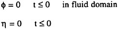
(10)
Numerical Method
As mentioned earlier, a solution to the above nonlinear initial boundary value problem is obtained using the Euler-Lagrange time-stepping procedure. The linear mixed boundary value problem for the perturbation potential is solved at each time step (using a desingularized boundary integral method) and the nonlinear free surface boundary conditions integrated in time. The body position and surface normal velocities are updated from the equations of motion of the vessel.
In the desingularized method, Rankine sources are distributed on an integration surface (Ω) that is offset from the physical problem boundary by a small distance. The potential anywhere in the fluid domain can then be calculated, in an indirect application of Green’s theorem, by integrating the influences of all the sources:
(11)
where ![]() is a point in the fluid domain,
is a point in the fluid domain, ![]() is a point on the integration surface,
is a point on the integration surface, ![]() is the strength of the source located at
is the strength of the source located at ![]() and
and ![]() is the Rankine source Green function. The Green function for three-dimensional problems is
is the Rankine source Green function. The Green function for three-dimensional problems is
(12)
An application of the appropriate Dirichlet and Neumann boundary conditions to (11) yields the integral equations that must be solved for the unknown source strength ![]() at each time step:
at each time step:
(13)
(14)
where ![]() is the given potential at
is the given potential at ![]() ΓD is the boundary on which
ΓD is the boundary on which ![]() is known, χ is the given normal velocity on the solid boundaries, and ΓΝ are surfaces on which χ is known. For isolated sources, the above integral equations become simple summations; when discretized over a total of Ν collocation points
is known, χ is the given normal velocity on the solid boundaries, and ΓΝ are surfaces on which χ is known. For isolated sources, the above integral equations become simple summations; when discretized over a total of Ν collocation points ![]() they result in an N×N linear system of the form
they result in an N×N linear system of the form
(15)
where: the influence matrix  for collocation points on the free surface and
 ![]() for collocation points on solid boundaries; σi is the vector of unknown source strengths; and bi is the vector of boundary conditions—for boundaries
for collocation points on solid boundaries; σi is the vector of unknown source strengths; and bi is the vector of boundary conditions—for boundaries ![]() on which the Dirichlet condition is prescribed (e.g., the free surface),
on which the Dirichlet condition is prescribed (e.g., the free surface), ![]() on the body surface, and bi=0 on a flat bottom. A variety of options have been exercised for the solution of this system of equations. These are the use of LU decomposition for the smallest problems (mostly two-dimensional); the use of the iterative solver, GMRES [Saad and Schultz (14)], for larger (three-dimensional, especially) problems; and, more recently, the incorporation of multipole acceleration techniques [Scorpio et al. (9)] to reduce the computational burden to O(N). Once the integral equations are solved for σj, hence
on the body surface, and bi=0 on a flat bottom. A variety of options have been exercised for the solution of this system of equations. These are the use of LU decomposition for the smallest problems (mostly two-dimensional); the use of the iterative solver, GMRES [Saad and Schultz (14)], for larger (three-dimensional, especially) problems; and, more recently, the incorporation of multipole acceleration techniques [Scorpio et al. (9)] to reduce the computational burden to O(N). Once the integral equations are solved for σj, hence ![]() the fluid velocities can be found using
the fluid velocities can be found using
(16)
without the need for numerical derivatives.
Finally, the free surface boundary conditions, (7) and (9), are integrated in time using the fourth-order Runge-Kutta method to obtain new values of
![]() and
and ![]() and the cycle is repeated. A steady-state solution is obtained by accelerating the vessel from rest up to steady forward speed.
and the cycle is repeated. A steady-state solution is obtained by accelerating the vessel from rest up to steady forward speed.
GEOMETRY PROCESSOR
The geometry processor was developed to enable UM-DELTA to handle arbitrary and complex hull forms easily and efficiently. Christened HULLGEO, the geometry processor can handle in addition to conventional raked bows and cruiser sterns, bulbous bows, sterns with deadwood, and transom sterns. It can also be extended easily to multihulls or tunnel hulls.
The underlying idea is of using precomputed cubic spline fits of the waterlines and stations to return values of the unit normals at the desired node locations. Figure 2 shows the unit normals returned by HULLGEO for the DDG5415 naval combatant model. The unit normals have been evaluated at test nodes distributed along the stations that formed the input to the processor. As can be seen clearly, the vectors closely represent the complex geometric features of the combatant.
Given that the normals are evaluated based on cubic spline fits, some amount of noise in the results is inevitable, especially if the body surface is coarsely discretized. The noise may be minimized by providing as input to HULLGEO a discretized surface of fine resolution; then, at the interface between HULLGEO and UM-DELTA, a select subset of the input stations may be retained as the stations on which collocation points are actually distributed.
UM-DELTA’s calculations using HULLGEO have been verified by comparisons of the computed waves for the mathematical Wigley hull. In the results section are presented the newer results obtained for arbitrary and complex hulls by UM-DELTA.
BREAKING WAVE DAMPER
A greater challenge than the accurate and efficient modeling of the geometry to UM-DELTA has been finding ways to cope with breaking waves and spray in the fully nonlinear computations. In linear or higher-order expansion methods, the wave amplitudes can get unrealistically large without causing numerical difficulties. In fully nonlinear computations, however, wave breaking or spray formation at the body-free-surface intersection will cause the computations to stop promptly even though the difficulty may be confined to a small area such as the breaking bow wave. To overcome this difficulty we have been working on the local suppression of wave breaking and spray by absorbing energy using the free surface boundary conditions. Recently, on the basis of studies in a two-dimensional numerical wave tank, Subramani et al. (15) proposed a technique by which to absorb energy locally from waves that are about to break, thereby suppressing wave breaking.
The “local absorbing patch” model may be activated in two steps: 1) detecting the likely occurrence of the wave breaking, and 2) determining the appropriate amount of local damping so as to render reasonably realistic waves in the post-breaking regime. The likely incidence of wave breaking was detected by monitoring the local free-surface curvature; when the curvature exceeded a suitably prescribed threshold value, a local wave damper was activated in the vicinity of the wave crest where the threshold was exceeded. The actual damping was provided by applying an artificial pressure on the free surface in such a manner that the pressure would always take energy out of the waves. As demonstrated in (15). the technique has been successfully applied to the suppression of spray and wave breaking in the case of two-dimensional water waves. However, we have yet to determine the right form of the damper for three-dimensional calculations with forward speed.
RESULTS
Arbitrary Hulls
The Series 60, CB=0.6 parent hull form, for which extensive experimental data is available, was selected as the realistic, arbitrary hull on which to test first the extended UM-DELTA code. Calculations were performed for a ship advancing straight ahead in calm water at two Froude numbers (Fr), 0.25 and 0.316, and using two body discretizations—a coarse grid consisting of 26 stations and a finer grid consisting of 51 stations. The node density along a station was prescribed to be 10 nodes along a girth equal to the ship draft. The total number of nodes on the body was 344 for the coarse grid hull and 680 for the finer one.
The domain of the numerical wave tank for either case was bounded by an upstream end 0.5 times the ship length, L, ahead of the bow, with the tank extending for 0.75 L downstream of the stern and measuring 0.6 L across. The free-surface discretization corresponding to the coarse body grid was 58 nodes in the longitudinal direction and 11 nodes in the transverse direction; for the fine grid
case, it was 114×22. For the coarse body grid, the number of free-surface nodes ahead of the body, across the body, and downstream of the body was, respectively, 13, 26, and 19; and for the fine grid, the corresponding distribution was 25, 51, and 38. The time-step size chosen was Δt=0.1, sufficiently small to ensure a stable time-integration.
Figure 3 shows a perspective view of the free-surface at steady state from a Fr=0.316 calculation on the finer grid. Note that due to symmetry, the calculations are performed in the half-domain, Y>0. The entire domain is depicted in figure 3 for illustrative purposes. The computed wave profile along the hull at Fr=0.25 for the two different discretizations considered is presented in figure 4 and compared with the experimental measurements of Toda et al. (16). The differences in the results for the two different grids are small and the calculations show reasonably good agreement with the data. However, clear differences exist, with an underprediction of the body-free-surface intersection, a shift in the bow wave crest, and a slightly overpredicted stern shoulder wave crest. The underprediction of the water-level at the bow is probably because of the thin sheet of fluid that shoots upward at the bow in reality and which is not easily captured in numerical methods. To some extent, the differences may also be due to the simplification of the Series 60, CB=0.6’s bow to a line bow of zero radius of curvature in the numerical method. Given the capability of HULLGEO to handle raked bows, the calculations could be repeated without the simplifications, in a more detailed study on the computed bow flow.
The computed wave profile along the hull at Fr=0.316 is presented next, in figure 5. In addition to the calculations for the two spatial discretizations considered, a fine grid calculation performed with a smaller time-step size of 0.05 is also presented and all the results are compared again with the data. The calculations show somewhat better agreement with the data, although the differences at the bow and at the stern shoulder wave crest persist. The differences in the results due to the different temporal discretizations are almost negligible; however, clear differences exist between the coarse and fine grid calculations due likely to inadequate resolution on the coarse grid. Owing to constraints on the available time, calculations with a still finer grid could not be made and shall be undertaken in the near future to complete the grid convergence study.
Figure 6, which presents a comparison of longitudinal wave-cuts with the available data—at Y/L=0.0755, 0.108, and 0.14108, for Fr=0.316—provides an indication of the accuracy of the computed wave field—the inviscid calculations are in very good agreement with the data over the length of the ship, except for a slight overprediction of the waves amidships.
The computational requirements for these calm-water calculations (steady state was attained at about t=25.0, accelerating gradually from rest) is as follows: the fine grid calculation required about 23 MW of memory and 2.5 hours on the CRAY C-90, while the coarse grid calculation attained steady-state in about 30 minutes of computer time on the same machine. Note that the high degree of vectorization within the UM-DELTA has it operating consistently over 500 MFLOPS on the C-90.
Finally, given that the UM-DELTA is a time-domain method for solving unsteady seakeeping problems, a preliminary calculation for the Series 60, CB=0.6 advancing in head seas is presented in figure 7. The calculation was performed on a coarse grid as described above (with 26 stations). The incident waves have an amplitude of about 0.006 L and a wavelength of about 1.0 L and they were turned on in the computation after the ship had accelerated from rest to steady forward speed, at Fr=0.25. Eventually, computations of the radiation and the exciting forces shall be presented for a range of Froude numbers.
Complex Hulls
One of the stated objectives for the current project is the calculation of the flow around complex hull forms such as naval combatants. The development of the HULLGEO module has made possible improvements to the UM-DELTA code that go precisely towards the meeting of this objective: enabling, for instance, an accurate resolution of the flow around bulbous bows by allowing a node to track the stem-free-surface junction as the water level rises or falls at the raked stem; allowing for nodes to be dropped or added in a robust manner and even for an entire station to be inserted at a new location, as necessary, depending on the change in the wetted portion of the hull.
However, additional extensions and modifications remain to be made to the code before results can be obtained for, e.g, the DDG5415 naval combatant model. This work is expected to be completed in the coming months. For the time being, we present here a calculation to demonstrate the capability of UM-DELTA for bulbous bows. The calculation was performed for a hull with a bulbous bow and a cruiser stern. The hull shape was created by fusing the forward half of the DDG5415 model with a cruiser stern whose lines were extracted from the Series 60, CB=0.6 model and which was also closed in with deadwood.
Calm water results were obtained for this hull at Fr=0.25 using two different body discretizations—a coarse grid with 32 stations and a fine grid with 52 stations. The number of nodes on the body was 302 for the coarse grid and 492 for the finer grid. The free-surface grid, in a domain of identical proportions to that discussed for the Series 60, CB=0.6 calculation, had a distribution 67×13 for the coarse grid run and 108×21 for the fine grid run. The calculated wave profile along the hull, for the forward portion of the hull—the portion of interest—is presented in figure 8. The differences between the calculations on the two grids are considerable and further calculations need to be performed to ensure grid convergence. However, this calculation was intended only to demonstrate the successful handling of a bulbous bow, before the initiating of calculations for a naval combatant model with a transom stern too. A technique for handling the flow characteristics of transom sterns has been devised from a two-dimensional study which is described in the next section.
2D TRANSOM STERN FLOW
To provide a starting point for the extension of the method to unsteady, fully nonlinear, three-dimensional transom stern flows, Scorpio and Beck (17) recently investigated, using the UM-DELTA method, the unsteady flow past a two-dimensional, semi-infinite body with a transom stern (unsteady in the sense that the problem was started from rest and accelerated to steady forward speed). To aid in the present discussion, the relevant material is discussed again here in some detail.
The cases studied by them corresponded to those in Vanden-Broeck and Tuck (18) and Vanden-Broeck (19), wherein nonlinear waves behind a transom stern were computed using a series expansion in the Froude number. In (18) and (19), the problem was solved in an inverse manner using the x and y coordinates as the dependent variables and the velocity potential and stream function as the independent variables. The series expansions in x and y were everywhere divergent but could be summed by standard methods. Integro-differential equations with nonlinear boundary conditions were solved in the inverse space to obtain the expansion coefficients.
Problem Formulation
Figure 9 shows the problem configuration. The x-y coordinate system is translating with speed Ub in the negative x-direction. Laplace’s equation governs in the fluid domain and the velocity potential is ![]() . The surfaces bounding the fluid are:
. The surfaces bounding the fluid are:
SF=Free Surface;
SH=Body Surface;
SU=Upstream Truncation Surface;
SD=Downstream Truncation Surface; and
SB=Bottom Surface.
The boundary conditions are:
(17)
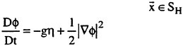
(18)
(19)
(20)
Here, ![]() is the material or Lagrangian derivative,
is the material or Lagrangian derivative, ![]() are the coordinates of control points on the problem boundary,
are the coordinates of control points on the problem boundary, ![]() is the unit normal on the body pointing out of the fluid, g is the acceleration of gravity, η is the free surface elevation, and
is the unit normal on the body pointing out of the fluid, g is the acceleration of gravity, η is the free surface elevation, and ![]() is the perturbation potential. The boundaries SU and SD are unspecified. Cases have been run with SU and SD prescribed to satisfy continuity and very little differences seen in the results as long as SU and SD are far enough up- and down-stream, respectively. The truncation boundaries were placed about 12 wavelengths away from the transom for these calculations.
is the perturbation potential. The boundaries SU and SD are unspecified. Cases have been run with SU and SD prescribed to satisfy continuity and very little differences seen in the results as long as SU and SD are far enough up- and down-stream, respectively. The truncation boundaries were placed about 12 wavelengths away from the transom for these calculations.
Results
Vanden-Broeck (19) suggested that two realistic solutions exist for the steady flow behind a transom stern. For small values of the Froude number, the flow rises up the transom to a stagnation point. The free surface separates from the transom at the stagnation point, creating waves downstream that increase in steepness with increasing Froude number. This solution will be referred to as “A” hereafter. Solution A is physically unreasonable for large Froude numbers because the ratio of stagnation height to transom depth goes to infinity as Froude number goes to infinity. For large Froude numbers a second, more physically realizable solution exists where the
flow separates cleanly from the bottom of the transom. This solution will be referred to as “B” hereafter. Solution Β reduces to the uniform stream as Froude number tends to infinity and the downstream waves steepen as Froude number becomes small. In fact, Vanden-Broeck found a minimum Froude number (=2.26) below which the downstream waves exceed the theoretical breaking wave steepness limit (2a/λ=0.141).
The problem is started from rest and the hull is accelerated up to steady forward speed. Using the UM-DELTA method, the inviscid solution always tends towards solution A as the hull reaches steady forward speed, regardless of the Froude number. In a viscous fluid, we know that the flow behaves like solution A at low Froude numbers and transitions to solution Β as Froude number increases. As the hull speed increases from rest, the flow separating from the bottom of the transom becomes turbulent, resulting in the “dead water” region commonly observed behind transom sterns. Consequently, the pressure behind the transom is lowered. Eventually the falling pressure causes the free surface to drop to the bottom of the transom resulting in the solution Β flow. Once the free surface separates cleanly from the transom, the turbulence is confined to a thin boundary layer (for high speeds) and the viscous wake. Using an inviscid flow model, it appears to be impossible to proceed from transom wetted to transom dry because of the lack of turbulence. However, two techniques were found by which to transition artificially the solution from A to B.
In the first method, the problem is started at steady forward speed with the transom out of the water. The hull is then slowly lowered into the water. As the hull is lowered, the free surface remains separated from the bottom of the transom and solution Β results. However, this technique will not work for a problem starting from rest with the transom immersed. To obtain solution Β for the problem starting from rest, a second technique was tried, attempting to mimic the effect of the dead water region by artificially lowering the stagnation pressure on the transom. This pressure drop can be modeled in the inviscid flow code by modifying the boundary condition on the transom. The condition,
(21)
causes the stagnation pressure. The technique consists of reducing the stagnation pressure by modifying the transom boundary condition to:
(22)
This modified form of the transom boundary condition was chosen arbitrarily. There is no special significance in the exponential decay other than it provides a smooth transition for the boundary condition. As the hull accelerates up to speed, the pressure on the transom drops until the free surface drops to the bottom of the transom. When the hull reaches steady speed, solution Β is recovered.
The general numerical details are similar to those outlined for the three dimensional problem. There is a double node where the free surface meets the transom in the solution A flow. One node satisfies the body boundary condition while the other satisfies the free surface boundary condition. Treating the intersection in this manner has consistently worked well in the desingularized method. There is one additional constraint (or Kutta condition) at the bottom of the transom in the solution Β flow. The free surface nodes move downstream with the fluid velocity during the intermediate time steps (4th order Runge-Kutta). At the end of a major time step the free surface nodes are regridded to their original positions by interpolating elevations and potentials. The Kutta condition is imposed by regridding the first free surface node back to the bottom of the transom. The potential at this point is computed from the source strengths.
Figure 10 shows the waves generated by the transom stern at ![]() . Figure 11 shows wave steepness versus Froude number for the waves downstream of the transom. The lines on the graph represent the relationship between wave steepness and Froude number derived by Vanden-Broeck (19). The Froude number can be related to the mean potential and mean kinetic energy in the wave train by integrating the momentum equation. The mean potential and kinetic energy are in turn functions of the wave steepness. The points represent results from the UM-DELTA method for various Froude numbers. Excellent agreement with the theoretical wave steepness is shown over a broad range of Froude numbers.
. Figure 11 shows wave steepness versus Froude number for the waves downstream of the transom. The lines on the graph represent the relationship between wave steepness and Froude number derived by Vanden-Broeck (19). The Froude number can be related to the mean potential and mean kinetic energy in the wave train by integrating the momentum equation. The mean potential and kinetic energy are in turn functions of the wave steepness. The points represent results from the UM-DELTA method for various Froude numbers. Excellent agreement with the theoretical wave steepness is shown over a broad range of Froude numbers.
CONCLUDING REMARKS
A multipole-accelerated, desingularized boundary integral method, UM-DELTA, has been developed over the past several years to solve fully nonlinear water-wave problems including wave loads on offshore structures and nonlinear ship motions. To date, the UM-DELTA method has been successfully applied to a wide variety of problems. However, the applications thus far have been limited to simplified body shapes such as spheroids, cylinders, and the
mathematical Wigley hull. An efficient and robust geometry processor was therefore developed to enable the handling of arbitrary and complex hull forms. The extensions of the method to realistic hull forms, with the incorporation of this geometry processor, is described herein.
Results are presented for the Series 60, CB=0.6 advancing in calm water for two different Froude numbers. The calculated wave profile and wave cuts are shown to be in good agreement with the experimental data. The method is also successfully demonstrated for a ship with a bulbous bow (modeled after the DDG5415 naval combatant model’s bulbous bow). However, work is still ongoing on extensions of the method to ships with transom sterns.
To aid in these extensions, a numerical investigation of unsteady, two-dimensional inviscid transom stern flow was recently carried out. The numerical results were shown to agree well with theory. Further, a technique for effecting the transition from transom wetted to transom dry at high Froude number, by artificially modifying the transom boundary condition, was successfully implemented. Additionally, it was seen that a transom dry solution could be maintained by regridding the first free-surface node back to the bottom of the transom at each step, with no other requirements.
Besides the continued extensions and improvements to the method, future work involves firstly the carrying out of additional, fine grid simulations to demonstrate better grid convergence; and equally importantly, the devising of ways in which to suppress the disruptive effects of spray and wave breaking in the fully nonlinear ship wave computations.
ACKNOWLEDGMENTS
This research was funded by the Office of Naval Research and the University of Michigan/Sea Grant/Industry Consortium on Offshore Engineering. The computations were made in part using an allocation of high performance computing resources through the National Partnership for Advanced Computational Infrastructure and through the Department of Defense High Performance Computing Modernization Program.
REFERENCES
(1) Jensen, G., Bertram, V., and Soding. H., “Ship Wave-Resistance Computations,” Proceedings, 5th International Conference on Numerical Ship Hydrodynamics, Hiroshima, Japan, 1989, pp. 593–606.
(2) Kim, Y.-H. and Lucas, T., “Nonlinear Ship Waves,” Proceedings, 18th Symposium on Naval Hydrodynamics, Ann Arbor, Michigan, 1990, pp. 439–452.
(3) Kim, Y.-H. and Lucas, T., “Nonlinear Effects on High Block Ship at Low and Moderate Speed,” Proceedings, 19th Symposium on Naval Hydrodynamics, Seoul, Korea, 1992, pp. 43–52.
(4) Raven, H.C., “A Practical Nonlinear Method for Calculating Ship Wavemaking and Wave Resistance,” Proceedings, 19th Symposium on Naval Hydrodynamics, 1992, pp. 349–370.
(5) Scullen, D.C. and Tuck, E.O., “Nonlinear Free-Surface Flow Computations for Submerged Cylinders,” Journal of Ship Research, Vol. 39, No. 3, 1995, pp. 185–193.
(6) Scullen, D.C., “Accurate Computation of Steady Nonlinear Free-Surface Flows,” Ph.D. Thesis, Department of Applied Mathematics, University of Adelaide, Feb. 1998)
(7) Longuet-Higgins, M.S. and Cokelet, E.D., “The Deformation of Steep Surface Waves on Water: I. A Numerical Method of Computation,” Proceedings, Royal Society of London,” Vol. A350, 1976, pp. 1–26.
(8) Beck, R.F., “Fully Nonlinear Water Wave Computations Using a Desingularized Euler-Lagrange Time-Domain Approach,” Nonlinear Water Wave Interactions, Computational Mechanics Publishers, U.K., 1998 (to appear).
(9) Scorpio, S.M., Beck, R.F., and Korsmeyer, F.T., “Nonlinear Water Wave Computations Using a Multipole Accelerated, Desingularized Method,” Proceedings, 21 Symposium on Naval Hydrodynamics, Trondheim, Norway, 1996, pp. 69–74.
(10) Cao, Y., Beck, R.F., and Schultz, W.W., “Numerical Computations of Two-Dimensional Solitary Waves Generated by Moving Disturbances,” International Journal of Numerical Methods in Fluids. Vol. 17, 1993, pp. 905–920.
(11) Beck, R.F., Cao, Y., Scorpio, S.M., and Schultz, W.W., “Nonlinear Ship Motion Computations Using the Desingularized Method,” Proceedings, 20th Symposium on Naval Hydrodynamics, Santa Barbara, August 1994, pp. 227–246.
(12) Scorpio, S.M. and Beck, R.F., “A Multipole Accelerated Desingularized Method for Computing Nonlinear Wave Forces On Bodies,” Journal of Offshore Mechanics and Arctic Engineering, Jan. 1998.
(13) Celebi, M.S. and Beck, R.F., “Geometric Modeling for Fully Nonlinear Ship-Wave Interactions,” Journal of Ship Research, Vol. 41, No. 1, 1997, pp. 17–25.
(14) Saad, Y. and Schultz, M.H., “GMRES: A Generalized Minimal Residual Algorithm for Solving Nonsymmetric Linear Systems,” SIAM Journal of Scientific and Statistical Computing, Vol. 7, 1986, pp. 856–869.
(15) Subramani, A.K., Beck, R.F., and Schultz, “Suppression of Wave-Breaking in Nonlinear Water Wave Computations.” Proceedings, 13th International Workshop and on Water Waves and Floating Bodies, Alphen aan Rijn, Netherlands, 1998.
(16) Toda, Y., Stern F., and Longo, J., “Mean-Flow Measurements in the Boundary Layer and Wake and Wave Field of a Series 60, CB=0.6 Ship Model—Part 1: Froude Numbers 0.16 and 0.316,” Journal of Ship Research. Vol. 36, No. 4, 1992, pp. 360–377.
(17) Scorpio, S.M. and Beck, R.F., “Two-Dimensional Inviscid Transom Stern Flow,” Proceedings, 12th International Workshop on Water Waves and Floating Bodies, Carry-le-Rouet, France, 1997.
(18) Vanden-Broeck, J.-M., “Nonlinear Stern Waves,” Journal of Fluid Mechanics. Vol. 96, No. 3, 1980, pp. 603–611.
(19) Vanden-Broeck, J.-M. and Tuck, E.O., “Computation of Near-Bow or Stern Flows, Using a Series Expansion in the Froude Number,” Proceedings, 2nd International Conference on Numerical Ship Hydrodynamics, Berkeley, California, 1977, pp. 371–381.
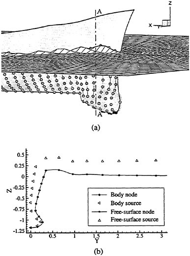
Figure 1. (a) Perspective view of typical grid distribution and (b) cross-section at A-A showing the relative locations of the nodes and sources
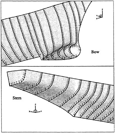
Figure 2. Unit normals on the body as obtained by the geometry processor: (top) bow and (bottom) stern regions of the DDG5415 combatant model
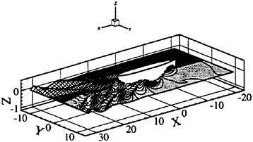
Figure 3. Perspective view of the steady-state free-surface for the Series 60, CB=0.6 at Fr=0.316 (114×22 free-surface grid, 680 body nodes)
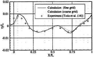
Figure 4. Wave profile along the hull for the Series 60, CB=0.6 at Fr=0.25 (Δt=0.1)
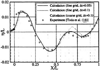
Figure 5. Wave profile along the hull for the Series 60, CB=0.6 at Fr=0.316
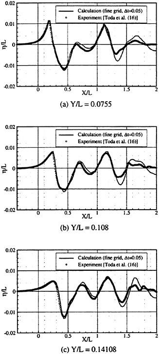
Figure 6. Longitudinal wave cuts for the Series 60, CB=0.6 at Fr=0.316
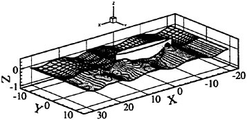
Figure 7. Perspective view of the Series 60, CB=0.6 advancing into incident waves of amplitude, 0.006 L and wavelength, 1.0 L
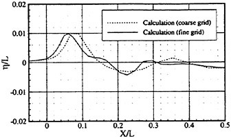
Figure 8. Wave profile along the hull (forward of midship) at Fr=0.25 for a ship with the bow of a DDG5415 combatant model
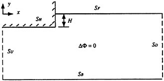
Figure 9. Problem configuration for 2D transom stern flow
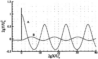
Figure 10. Waves generated by the 2D transom stern at a Froude number based on transom depth of FH=6.3
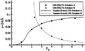
Figure 11. Wave steepness versus Froude number, FH for waves downstream of the transom
DISCUSSION
H.Haussling
Naval Surface Warfare Center, Carderock Division, USA
The authors have made substantial progress on extending a method for the computational solution of inviscid nonlinear water wave problems to more realistic hull shapes than they previously considered. To aid in this effort they have investigated the computational solution of inviscid two-dimensional transom stern flows and showed that their results compare favorably with the analysis of Vanden-Broeck. I would like to call attention to a computational investigation of the very same problem carried out 20 years ago at David Taylor Model Basin (1, 2), which the authors seem unaware of or at least don’t reference. This earlier work showed that solution Β can be attained through an unsteady formulation by assuming the free surface is fixed at the bottom of the transom for all time after an abrupt acceleration of the stern. The solution Β obtained was shown to agree with Vanden-Broeck. The instantaneous drop of the free surface to the transom bottom would seem to be similar to a very large β in the authors’ equation (22). This rapid drop seems a good model for fast hull accelerations where the transom is noted to become dry very quickly. This happens even at accelerations to low final speeds where the transom eventually becomes wet again after a large stern wave develops and spills forward.
The earlier work did not consider solution A because of its unreality. As pointed out by the authors, unlike solution A, a real low-speed flow will separate at the bottom of the transom, and there will be a recirculating eddy behind the hull. In fact, care must be taken not to assign too much reality to either of solutions A and Β (as might be implied by the first sentence in the Results section following equation (20)). It was shown some time ago that, while solution Β has a degree of reality beyond that of solution A, its breakdown at a depth Froude number of 2.26 has little bearing on the transition from wetted to dry transom flow (3). Its failure to capture the slowing of the flow in the boundary layer leads to significant errors in its prediction of the wave field (4). In the transom stern region the accuracy of potential flow predictions of the wave field is seriously degraded compared to other portions of the hull.
The authors included a discussion of the use of a free-surface pressure patch to control the deleterious effects of wave breaking on numerical computations. It might be mentioned that this approach was also first suggested and used successfully at David Taylor Model Basin some time ago (5).
References
(1) Haussling, H.J., “Two-Dimensional Linear and Nonlinear Stern Waves,” Journal of Fluid Mechanics, Vol. 97, part 4, 1980, pp. 759–769.
(2) Coleman, R.M. and Haussling, H.J., “Nonlinear Waves Behind an Accelerated Transom Stern,” Proceedings, 3rd International Conference on Numerical Ship Hydrodynamics, Paris, June 1981.
(3) O’Dea, J., Jenkins, D., and Nagle, T., “Flow Characteristics of a Transom Stern Ship,” David W.Taylor Naval Ship Research and Development Center Report 81/1057, 1981.
(4) Haussling, H.J., Miller, R.W., and Coleman, R.M., “Computation of High-Speed Turbulent Flow About a Ship Model With a Transom Stern,” Carderock Division, Naval Surface Warfare Center Report CRDKNSWC/HD-0200–51, September, 1997.
(5) Haussling, H.J. and Coleman, R.M., “Nonlinear Water Waves Generated by an Accelerated Circular Cylinder,” Journal of Fluid Mechanics, Vol. 92, part 4, 1979, pp. 767–781.
AUTHORS’ REPLY
We thank Dr. Haussling for his comments and for calling our attention to the works mentioned. We intended our two-dimensional transom stern study to serve only as a validation of our numerical approach against Vanden-Broeck’s calculations; our omission of references (1) and (2) was solely the result of oversight. The important part of our study is the methodology for enabling a transition from a wetted to a dry transom, a methodology that we may extend to three-dimensional transom sterns.
We recognize the shortcomings of the inviscid formulation for flow behind a transom stern. We do not mean to suggest that the solution A flow or transition flow is at all realistic. However, we note that the inviscid flow appears to be more realistic for solution B as Froude number increases.
We are also thankful to be made aware of Haussling and Coleman (5). However, we would like to clarify that the work does not elaborate on the basis for the criterion chosen therein for the triggering of the pressure patch damper. Our work on the development of this approach differs in this regard.
Fully Nonlinear Interactions of Long-Crested Wave Packets with a Three-Dimensional Body
P.Ferrant (Societe d’Ingenierie et de Recherche en Hydrodynamique Navale, France)
ABSTRACT
In this paper we describe a fully non linear time domain diffraction model for free surface potential flow. The originality and power of the method lie in the separation of incident and diffracted non linear flows, based on the availability of explicit models for the incoming waves. With some hypotheses on the incoming wave model, a formulation of the problem in terms of the fully nonlinear diffracted potential and wave elevation is obtained. Recent validation results, with comparison to experiments or higher order diffraction models are presented, in the case of regular incoming waves with or without current, and assess the accuracy and flexibility of the present diffraction model. Then the issues associated to the extension of the model to irregular waves are discussed, and a solution method for short duration wave packets interacting with a three dimensional body is described.
INTRODUCTION
In recent years considerable efforts have been devoted to the development of fully non linear simulation methods for wave-body interactions, aiming at practical application both in naval and offshore industries. This approach is now quite popular in its two dimensional implementation. However, despite continuing advances both in hardware and numerical methods, the applications of direct three dimensional fully non linear models for wave-body interaction problems remain limited and require considerable computing ressources for reasonably accurate results (Celebi et al 1998). At an intermediate level of complexity and computing demand, the time domain second order approximation of the fully non linear problem may represent a valuable alternative in moderately steep regular waves, see e.g. Isaacson & Cheung (1992), Skourup et al (1997), or Kim et al (1998), but misses significant nonlinear features of the diffraction phenomenon when applied to steep transient wave packets (Ferrant & Guillerm 1998).
The fully non linear model described in this paper is based on an original approach in which an explicit description of the non linear incident wave is exploited. The problem is then formulated for the diffracted wave, without restriction on non linearities.
In the case of regular incoming waves without current, the incoming flow is represented by a stream function model (Rienecker & Fenton 1981). Significant results in this case have already been published (Ferrant 1996), and we give here extended validation results, with comparison to recent experiments from University of Oslo (Huseby & Grue 1998) for higher harmonic wave loads. In regular waves plus current, extensive results may be found in Ferrant (1998), with a parametric study on the combined non linear influence of wave steepness and current strength on the wave runup about a vertical cylinder. A comparison with experimental runup data from Ifremer (Le Noac’h et al 1997), both with and without current, is presented in the present paper. These results attest the accuracy and versatility of the nonlinear diffraction formulation, in the case of nonlinear regular waves with or without current.
At last, the issues associated to the extension of the present model to irregular incoming waves are discussed, and a solution method for short duration non linear long-crested wave packets interacting with a three-dimensional body is described.
THEORETICAL FORMULATION
Semi-Lagrangian formulation
We consider a three-dimensional fluid domain (D), bounded by a free surface F and a set of N solid boundaries Si. These boundaries include the surface of a fixed offshore structure, as well as the sea floor at finite distance. The domain is of infinite extent in the horizontal directions. The fluid flow problem is formulated in the frame of potential flow
theory. The fluid velocity thus derives from a scalar potential satisfying Laplace’s equation at any point of the fluid domain:
(1)
(2)
On the free surface, both kinematic and dynamic conditions must be satisfied. The kinematic condition states that the mass flux through the free surface is zero, and writes, in Lagrangian form:
(3)
If surface tension is ignored, the dynamic condition expresses the continuity of the pressure across the free surface, and derives from Bernoulli’s equation:
(4)
where D/Dt stands for the material derivative. Equations (3) and (4) suppose a fully Lagrangian description of the free surface, with markers identified as material points. In the present paper, the formulation will be modified by inhibiting the horizontal motions of free surface markers, leading to a semi-Lagrangian description. In such a formulation, the free surface vertical co-ordinate becomes implicitly single-valued, and may be expressed as:
(5)
Plugging this notation into (3) and (4), and after some manipulations, we obtain new forms of the non-linear kinematic and dynamic boundary conditions, in which a fixed projection of free surface markers in the x-y plane is implied:
(6)
(7)
where η is the free surface elevation, z is positive upwards with its origin on the mean position of the free surface. Non dimensional quantities are assumed, based on a reference length L and with the acceleration of gravity g as the acceleration of reference. In the present paper, L is the water depth h.
On fixed material boundaries, no-flux Neumann conditions are applied:
(8)
Separation of an explicit part of the solution
In some situations, it is practical to re-formulate the general problem described in the preceding section, by substracting from the total flow a contribution which may be explicitly described. The aim of such a procedure is to be left with a modified problem for the remaining part of the flow which will be easier to solve. This is what is usually achieved in linearized radiation-diffraction theory when prescribing the incident wave potential and solving the problem for the diffracted flow alone. Here the situation is sensibly more complicated, since the boundary-value problem is non linear. However, the field equation itself, namely Laplace’s equation, remains linear so that we may write:
(9)
where Φe is a scalar potential satisfying Laplace’s equation in the whole fluid domain. In the same manner, in a single-valued description of the free surface, we may write:
(10)
where ηe is some explicit time dependent function of the horizontal co-ordinates. Plugging (9) and (10) into (6) and (7), we are left with free surface conditions for Φd and ηd, in which terms depending on Φe and ηe are supposed to be evaluated explicitly.
(11)
(12)
Note that at this point, Φd and ηd are totally independent of each other, the only constraint is on Φd which must satisfy Laplace’s equation throughout the fluid domain.
Specification of the incoming flow
In the present study, the incoming flow is composed either of a uniform current superimposed to non linear regular waves, or of short duration wave packets.
In the former case, the incident wave is modelized by a stream function model (Rienecker & Fenton, 1981). The model for wave packets is discussed in the sequel of this paper. In the stream function model, which is valid for both deep and shallow water, the velocity potential and elevation of a periodic wave traveling over a horizontal bottom are expressed as Fourier series. Nonlinear free surface conditions are satisfied exactly at some equidistant points distributed over one wave length, so that the error in the solution is driven by the truncation of the Fourier series only. The incident wave elevation is given by:
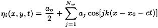
(13)
and the potential by:
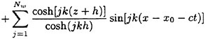
(14)
where U is the current speed, c the wave celerity, k the wave number and Nw the order of truncation of the Fourier series. The incoming flow being specified, conditions at infinity simply write:
(15)
Formulation for the perturbation flow
The most evident choice for Φe is Φi, simply by examining the simplification induced on the condition at infinity, and the fact that after this choice, a major contribution to the total flow will be represented analytically, with advantages in terms of global accuracy. For identical reasons, we shall also adopt ηe=ηi. The resulting boundary value problem to be solved for (Φd, ηd) is thus:
(16)
On the free surface (z=η(χ, y, t)), kinematic and dynamic boundary conditions become:
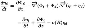
(17)
and:
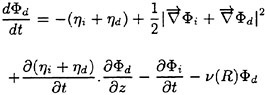
(18)
In these equations, ![]() stands for
stands for ![]()
![]() and terms involving Φi and ηi will be evaluated exactly from the stream function model. Damping terms involving functions ν(R) have also been included. The role of these terms is to absorb the diffracted waves on the outer part of the free surface mesh. More details on the implementation of this absorbing zone technique are given in a following section.
and terms involving Φi and ηi will be evaluated exactly from the stream function model. Damping terms involving functions ν(R) have also been included. The role of these terms is to absorb the diffracted waves on the outer part of the free surface mesh. More details on the implementation of this absorbing zone technique are given in a following section.
Initial conditions in the domain correspond to the incident wave without perturbation:
(19)
On the body, the no-flux conditions will be written:
(20)
where α(t) is a smooth ramp function varying from 0 to 1 during the beginning of the simulation (typically 1 to 2 wave periods). It must be emphasized that the boundary-value problem being non-linear, equations (17) and (18) will be satisfied on the instantaneous free surface position, so that the incident potential Φi may possibly be evaluated above the undisturbed incident wave z=ηi(x, y, t). This is possible here because the stream function potential has a continuous prolongation above the incident wave. One of the advantages of this formulation is that the incident wave is treated explicitly, so that it is not altered during its propagation from the outer surface of the computational domain to the body. In addition, the perturbations represented by (Φd, ηd) are composed of waves propagating in radial directions, allowing relatively coarse meshes to be adopted far from the body, in the absorbing zone. This results in considerable savings of memory and CPU time, without loss of accuracy. On the other hand, this formulation is not universal and rely on the availability of an explicit model for the incident wave, with appropriate continuity properties across the incident wave The initial boundary problem being properly posed, a solution procedure based on a boundary integral equation method is set-up. Applying Green’s identity to the velocity potential and to the free space Green function (Rankine source) G(M, Μ′)=−1/4πΜΜ′, we
obtain an integral representation of the velocity potential Φd:
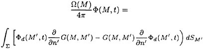
(21)
where Ω(Μ) is the internal solid angle at point Μ. Ω(Μ)=2π for Μ on the fluid boundary surface S, and Ω(Μ)=4π in the fluid domain. Applying a Dirichlet condition on the free surface and Neumann conditions on the rest of the fluid boundary, we are left with a mixed Fredholm integral equation of the first kind on the free surface, and of the second kind elsewhere. This equation will be solved at fixed time t for ∂Φd/∂n. The solution procedure adopted to solve the initial boundary value problem pertains to the family of mixed Euler-Lagrange methods and involve a combination of numerical schemes described in the following section.
NUMERICAL METHODS
Boundary element method
A boundary element method is used for the solution of the boundary integral equation formulation of the problem. The method is based on iso-parametric triangular elements distributed over the different boundaries. A piecewise linear, continuous variation of the solution over the boundary is thus assumed, and collocation points are placed at panel vertices. Meshes are made of an assembly of different patches, with the assumption of continuous normal on each of them. On intersection lines between two patches, two collocation points are considered for one single geometrical location, and the boundary conditions corresponding to the two surfaces are both satisfied. This discretization scheme reduces the integral formulation to a linear algebraic system to be solved for the normal velocity on Dirichlet boundaries (free surface) and the potential on Neumann boundaries. This system is assembled from the influence coefficients of linearly varying distributions of sources and dipoles on boundary elements. Analytical formulas for the near field, and different approximate formulas for the intermediate and far field are implemented. These coefficients are factorized with respect to sources or dipoles density at panel vertices, which are selected as control points. This scheme results in full, non-symmetric square systems of equations to be solved for the singularity distributions at the boundaries of the computational domain.
Solution of linear systems of equations
In 3D non linear applications large systems of equations have to be solved at each time step, and any O(N3) solution algorithm is absolutely unsuitable. In the present formulation, the linear systems to be solved are full and non-symmetric. The GMRES scheme of Saad & Schultz (1983) is applied to the solution of these systems. The method is used with diagonal pre-conditioning, which reduces the necessary number of iterations by a factor close to 2, at no additional cost. Further reductions of the number of iterations may be obtained with more elaborate pre-conditioning techniques, but the cost of such pre-conditionings applied to full matrices is not negligible and may annihilate the advantage of the reduction of the number of iterations.
Interpolations and smoothing at the free surface
In the present application, the projection of free surface nodes on the x-y plane is time-invariant, and the mesh is structured in the azimutal direction, that is nodes are distributed on circles surrounding the body, with a regular spacing on each circle. This situation allows us to apply a bi-cubic interpolation scheme for both the potential and the vertical co-ordinate at the free surface. These quantities are first interpolated at each radial station as functions of the azimutal angle. Then; interpolating splines are computed in the radial direction, at each free surface node. We are thus left with C2 representations of Φ and η at the free surface, which allow accurate and straightforward evaluations of the velocity components and of the normal vector, by direct differentiation of the interpolating splines. This procedure has proved to be sensibly more accurate than the local polynomial fitting used in the general case, but cannot directly be applied on arbitrary geometries. The structure of the free surface mesh is also exploited for the application of smoothing procedures at the free surface. This smoothing may become necessary for removing saw-tooth instabilities appearing during the simulation of strongly non-linear flows. Here we use five points formulas based on Chebyshev polynomials, applied sequentially in each parametric direction. For simulations presented in this paper, the smoothing proved necessary in the strongest cases, and was applied typically every five time steps.
Time marching scheme
After the solution of the boundary value problem and the computation of the fluid velocities and normal vector at the free surface, free surface conditions (17) and (18) considered as ODE for Φ and η are advanced in time. A fourth order Runge-Kutta scheme is used for that purpose, requiring four solutions of the boundary value problem per time step. In order to reduce CPU times, results presented in this paper were obtained using the “frozen coefficient” approximation, in which influence coefficients are updated only one time per time step, while four solutions of the boundary value problem are performed.
APPLICATIONS IN REGULAR WAVES
Wave loads on a vertical cylinder in long waves
In Huseby & Grue (1998), experimental data on wave loads about a thin vertical cylinder in long regular waves were presented, in the form of the harmonic coefficients of the steady-state horizontal force on the body. Harmonics up to the 3ω force were given, for a wave number kR=0.245 (R is the cylinder radius), and for different wave amplitudes. The present nonlinear diffraction model was run in similar conditions, and a very good agreement was observed on the amplitude and phases of experimental and numerical results. This motivated a deeper comparison, in which measured and simulated wave loads are compared up to the seventh harmonic (Grue & Huseby, private communication, 1998). The extended comparison is presented in this section. Regarding the details of the experimental procedure, we refer to Huseby and Grue (1998). Figures 1 to 7 present normalized amplitudes and phases of both numerical and experimental results, for kR=0.245, with respect to the wave amplitude Ak. The agreement is strikingly good in every respect. Only on the second harmonic force, an almost constant difference between simulations and experiments is observed. At small Ak, present non linear simulations results are very close to the asymptotic value of about 0.59 given by second order perturbation theory (Newman 1996), while both experiments and present fully nonlinear simulations capture the third order triple frequency loads predicted by Malenica & Molin (1995) Another remarkable result is the strong monotonic decay of higher harmonic force coefficients (especially F5, F6, F7) when the wave steepness increases. Note that the overlapping region of numerical and experimental results tends to shrink when going to higher harmonics. This is due to the difficulty of extracting very small parts of experimental time series for moderate amplitudes, while simulated results were limited to Ak=0.145, due to local instabilities appearing at the cylinder waterline for steeper incoming waves. The observed level of agreement is extremely satisfactory and is an indication of the reliability of both experimental and numerical models. Considering that the free surface mesh used in the present simulations is not supposed to correctly resolve waves shorter than 3ω free waves, such a level of agreement up to the 7ω force seems to indicate that higher harmonic forces are not linked to short diffracted free waves. This will be investigated in a forthcoming study.
Wave runup in regular waves and current
Here we compare results of the present nonlinear model to experiments performed by Ifremer (Le Noac’h et al, 1997). Regular waves are diffracted by a vertical cylinder of diameter 0.50 m and draft 1.25 m. The water depth in the Ifremer wave basin is 10 m. Three cases are presented here. The two first cases correspond to tests without current, with respectively T=2.066 s, H=0.30 m and Τ=2.582 s, Η=0.30 m, where Τ is the wavemaker motion period and Η is the incident wave height. Figures 8 and 9 give comparisons of simulated and measured runup time series about the cylinder, respectively at the upwave and downwave points of the cylinder waterline. Experimental data were obtained by video processing. The agreement is very satisfactory for both signals, the strong nonlinearity of the experimental signal being perfectly recovered by the numerical model. A similar agreement is observed for longer waves, T=2.582 s, H=0.30 m (figures 10 and 11). At last, a comparison involving a steady current superimposed to regular waves is depicted by figures 12 and 13. The wavemaker period is 2.582 s, the wave height is 0.30 m, and the current speed (simulated by a forward motion of the model in the experiments) is V=0.26 m/s. In figures 12 and 13, runup results obtained with a linearized time domain diffraction model are also given. Nonlinear effects are again nicely modeled by the fully nonlinear simulation, while the linearized model misses essential features of the experimental results, especially upwave.
EXTENSION TO NONLINEAR WAVE PACKETS
Principle
The key of the separation of incident and diffracted flows in the fully nonlinear diffraction model described above is the availability of a prolongation of the incident wave potential above the incident wave. In regular waves, the stream function allows the estimation of the incident wave potential and velocities below or above the incident wave without difficulty. When accounting for transient waves, things are sensibly more complex. One possible solution for representing the incident flow would be to run a two dimensional nonlinear time domain free surface model to obtain a transient nonlinear incident wave from a given wave maker motion time series. However, potential and velocities would have to be evaluated by some kind of extrapolation, which is not recommended when accurate results are expected. Another solution is adopted here. The entry of the process is the record of the incident wave packet at a specific location X0 on the free surface. The signal being bounded in time, the corresponding nonlinear incident flow can be reconstructed using a Fourier series expansion in space and time (Baldock & Swan 1994, Chaplin 1996). The coefficients of this double series are determined through the minimisation of an objective function based on the errors on kinematic and dynamic conditions in the vicinity of X0. The resulting representation of the incident wave packet is continuous across the incident free surface. The nonlinear diffraction model with separation of the incident potential and velocities may thus be applied, just as with the stream function model.
Description of test cases
The numerical model described above will be tested in realistic conditions corresponding to experimental tests run in 1994 in the frame of a french CLAROM project on ‘High frequency resonances of offshore structures’. A vertical cylinder model, supposed to reproduce a mini-GBS at scale 1:60, was placed in the towing tank of Ecole Centrale de Nantes. The distance between the wave maker and the model was 33 m, the water depth was 2.9 m, and various combinations of exciting waves and mechanical parameters were investigated. For more details on the experimental procedure, we refer to Scolan et al (1997). Among the available experimental results, we selected tests with short wave trains interacting with the cylinder rigidly fixed. Available data include wave forces and overturning moments, and wave elevation measured on the side of the cylinder, and have recently been compared with second order time domain simulations (Ferrant & Guillerm 1998). Although reducing the gap between first order and experimental quantities, the second order model was shown to miss some essential features of the nonlinear wave-body interactions, which motivated the extension of our non linear diffraction model to transient wave packets.
CONCLUSION
Extended validation results of a fully nonlinear diffraction model for regular waves with or without current have been presented and assess the validity and power of the underlying theory. The extension of the model to short duration nonlinear wave packets interacting with a three dimensional body is then described, as well as experimental tests with which comparisons are planned. Future work include further extension to long duration irregular incoming waves, possibly based on a local Fourier approximation for nonlinear irregular waves, along similar lines as described in Sobey (1992).
Acknowledgments: The development of the nonlinear free surface flow simulation model Answave has been supported by the French Ministry of Defense, through various research contracts. Recent developments were achieved in the frame of french CLAROM projects, funded by CEP&M. The author would like to thank Professor John Grue for valuable discussions and exchange of results. The help of IFREMER/DITI/GO/HA who supplied experimental runup values in waves and current is also greatly appreciated.
REFERENCES:
T.E.Baldock & C.Swan, ‘Numerical calculations of large transient water waves’, Applied Ocean Research, vol. 16, pp 101–102, 1994
B.Buchmann, J.Skourup, K.F.Cheung, ‘Runup on a structure due to waves and current’, ISOPE’97, Honolulu, 1997
M.S.Celebi, M.H.Kim, R.F.Beck, ‘Fully nonlinear 3D numerical wave tank simulation’, J.S.R., Vol. 42, 1, pp 33–45, 1998.
J.R.Chaplin, ‘On frequency-focusing Unidirectional waves’, Int. J. Offshore and Polar Engg., Vol. 6, 2, 1996.
P.Ferrant, ‘Simulation of strongly nonlinear wave generation and wave-body interactions using a 3D MEL
model’, 21st ONR Symposium on Naval Hydrodynamics, Trondheim, 1996.
P.Ferrant, ‘Runup on a cylinder due to waves and current: potential flow solution with fully nonlinear boundary conditions’, Proc. 8th Int. Conf. Offshore and Polar Engg, ISOPE’98, 1998
P.Ferrant & P.E.Guillerm, ‘Interaction of second order wave packets with a vertical cylinder’, Proc. 8th Int. Conf. Offshore and Polar Engg, ISOPE’98, 1998
J.Grue & M.Huseby, ‘Higher harmonic forces on a vertical cylinder’, Private communication 1998.
M.Huseby, J.Grue, ‘An experimental investigation of higher harmonic forces on a vertical cylinder in long waves’, Proc 13th Int. Workshop on Water Waves and Floating Bodies, Aalphen an den Rijn, 1998.
Isaacson, M, and Cheung, KF, “Time Domain Second Order Wave Diffraction in Three Dimensions”, J. Waterways, Port, Coast. And Ocean Engg., ASCE, Vol. 118, Part 5, 496–515., 1992
Y.Kim, D.C.Kring, P.D.Sclavounos, ‘Linear and nonlinear interactions of surface waves with bodies by a three dimensional Rankine panel method’ Appliead Ocean Research, Vol. 19, pp 233–249, 1998.
A.Le Noac’h, D.Buisine, M.Le Boulluec, ‘Surlvations de la houle autour d’un cylindre’, Ifremer Report DITI/GO/HA R11HA97, 1997.
S.Malenica, B.Molin, ‘Third harmonic wave diffraction by a vertical cylinder’, J. Fluid Mech., Vol. 302, pp 203–229, 1995.
J.N.Newman, ‘Second-order diffraction loads upon three dimensional bodies’, J. Fluid Mech., Vol. 320, pp 417–443, 1996
M.M.Rienecker, J.D.Fenton, ‘A Fourier approximation method for steady water waves’, J. Fluid Mech, Vol. 104, pp 119–137, 1981.
Y.Saad, M.H Schultz, ‘A generalized minimal residual algorithm for solving non-symmetric linear systems’, Res. Report Yale University RR-254, 1983.
Scolan, YM, Le Boulluec, M, Chen, XB, Deleuil, G, Ferrant, P, Malenica, S, and Molin, B, “Some Results from Numerical and Experimental Investigations on the High Frequency Responses of Offshore Structures”; Proc BOSS’97 Conference, Delft, The Netherlands, 1997.
Skourup, J, Buchmann, B, and Bingham, HB, “A Second Order 3D BEM for Wave-Structure Interactions”, Proc. 12th Int. Workshop on Water Waves and Floating Bodies, Carry-le-Rouet, France, 1997.
R.J.Sobey, ‘A local Fourier approximation method for irregular wave kinematics’, Applied Ocean Research, vol. 14, pp 93–105, 1992.
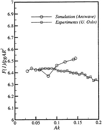
Figure 1-a: Inline force on a thin vertical cylinder in long waves: Amplitude of the 1st harmonic.
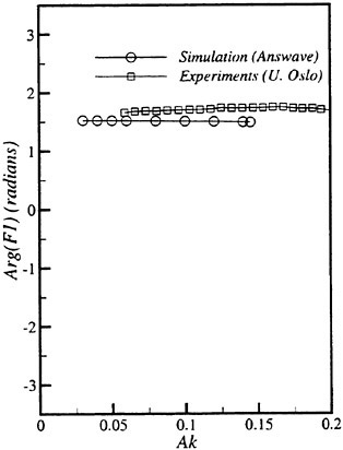
Figure 1-b: Inline force on a thin vertical cylinder in long waves: Phase of the 1st harmonic
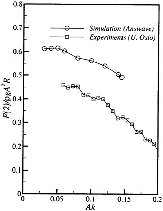
Figure 2-a: Inline force on a thin vertical cylinder in long waves: Amplitude of the 2nd harmonic.
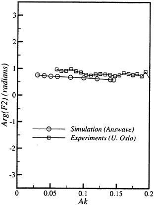
Figure 2-b: Inline force on a thin vertical cylinder in long waves: Phase of the 2nd harmonic
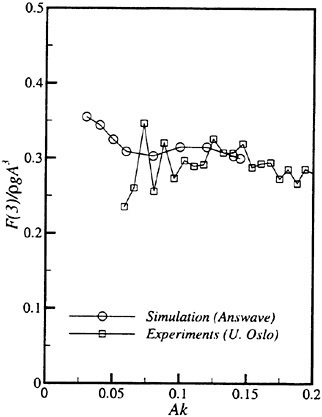
Figure 3-a: Inline force on a thin vertical cylinder in long waves: Amplitude of the 3rd harmonic.
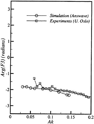
Figure 3-b: Inline force on a thin vertical cylinder in long waves: Phase of the 3rd harmonic.
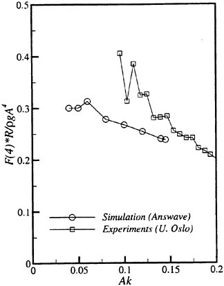
Figure 4-a: Inline force on a thin vertical cylinder in long waves: Amplitude of the 4th harmonic.

Figure 4-b: Inline force on a thin vertical cylinder in long waves: Phase of the 4th harmonic
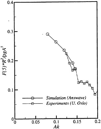
Figure 5-a: Inline force on a thin vertical cylinder in long waves: Amplitude of the 5th harmonic.
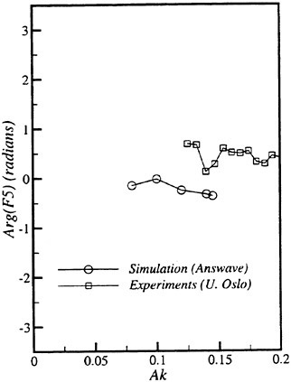
Figure 5-b: Inline force on a thin vertical cylinder in long waves: Phase of the 5th harmonic.
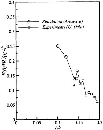
Figure 6-a: Inline force on a thin vertical cylinder in long waves: Amplitude of the 6th harmonic.
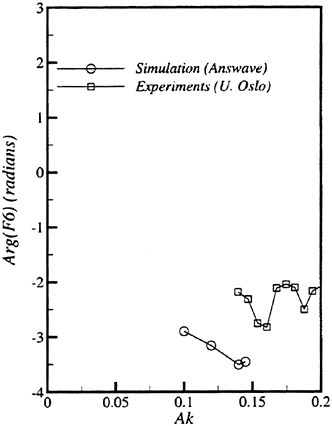
Figure 6-b: Inline force on a thin vertical cylinder in long waves: Phase of the 6th harmonic.
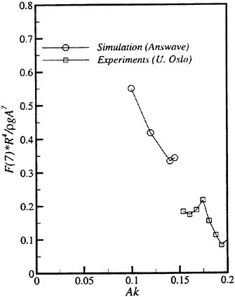
Figure 7-a: Inline force on a thin vertical cylinder in long waves: Amplitude of the 7th harmonic.
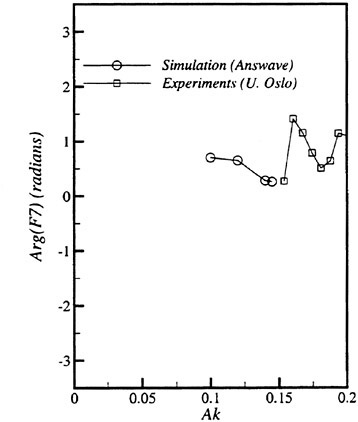
Figure 7-b: Inline force on a thin vertical cylinder in long waves: Phase of the 7th harmonic.
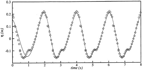
Figure 8: Vertical cylinder in waves and current. R=0.50 m; T=2.066 s; H=0.30 m; V=0.0 m/s. Runup Upwave. Solid line: Fully non linear simulation. Circles: Experiments Ifremer.
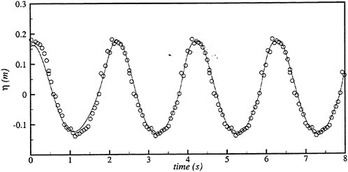
Figure 9: Vertical cylinder in waves and current. R=0.50 m; T=2.066 s; H=0.30 m; V=0.0 m/s. Runup Downwave. Solid line: Fully non linear simulation. Circles: Experiments Ifremer.
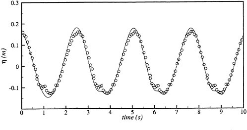
Figure 10: Vertical cylinder in waves and current. R=0.50 m; T=2.582 s; H=0.30 m; V=0.0 m/s. Runup Upwave. Solid line: Fully non linear simulation. Circles: Experiments Ifremer
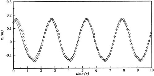
Figure 11: Vertical cylinder in waves and current. R=0.50 m; T=2.582 s; H=0.30 m; V=0.0 m/s. Runup Downwave. Solid line: Fully non linear simulation. Circles: Experiments Ifremer.
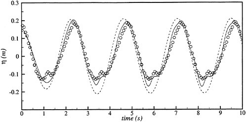
Figure 12: Vertical cylinder in waves and current. R=0.50 m; T=2.582 s; H=0.30 m; V=0.26 m/s. Runup Upwave. Solid line: Fully non linear simulation. Circles: Experiments Ifremer. Dashed line: linearized time domain wave+current model
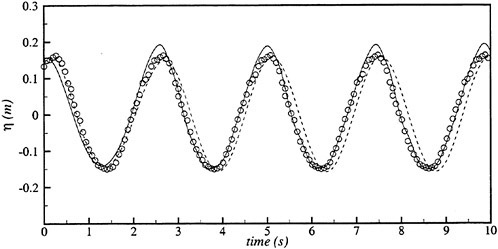
Figure 13: Vertical cylinder in waves and current. R=0.50 m; T=2.582 s; H=0.30 m; V=0.26 m/s. Runup Downwave. Solid line: Fully non linear simulation. Circles: Experiments Ifremer. Dashed line: linearized time domain wave+current model.
DISCUSSION
K.Thiagarajan
Australian Maritime Engineering, Australia
This discussion pertains to wave-current interaction experienced in a real environment. In the theoretical formulation current field and wave field are decoupled, and the only effect included is perhaps the Doppler shift in frequency. In the experiments, current is modeled by towing the cylinder in waves, and hence any interaction effects were not realized. The question is whether nonlinear interaction effects between waves and currents (e.g., change in wave height due to non-collinear currents) are important for the run-up problem presently considered, which is inherently nonlinear.
AUTHOR’S REPLY
The incident flow modeling used in the paper may seem simplistic, compared to what is needed when a depth-varying current is interacting with waves, possibly with different directions of propagation. However, this formulation is exact in the present case of symmetric non-linear regular waves superimposed to a uniform current. For a given wave number, accounting for a uniform current not only changes the frequency (Doppler shift effect), but also the mean mass flux. Both effects are included in the present formulation, and contribute to the non-linear interactions of waves and current with the fixed body. The only assumptions relate to potential flow and non-overturning waves. The model is continuously valid from the case of a uniform current without waves (equivalent to the non-linear wave resistance problem), to the case of regular waves without current (nonlinear diffraction problem). In the intermediate case of waves plus current, the problem treated is strictly equivalent to the case of a body with forward speed interacting with pure regular waves. This allowed us to compare our results with experiments with a model towed in waves, on the condition that the incoming frequency and wave number are the same in both the numerical and physical experiments.
Results show a sensible enhancement of the quality of runup estimations in waves plus current, compared to the most advanced Stokes expansion approaches. See for example reference [1] for a comparison of the present nonlinear formulation with a second order in wave steepness, first order in current speed, Stokes expansion formulation.
More complicated current configurations, such as the case of depth-varying currents common in coastal zones, are of course of interest, but in general lead to rotational flows for which the present potential flow theory is not valid.
DISCUSSION
U.Bulgarelli
Istituto Nazionale per Studi ed Esperienze di Architettura Navale, Italy
The free surface is allowed to move only vertically (z direction). Do you assume any regularity about the incident potential close to the free surface?
AUTHOR’S REPLY
In this paper, the fully nonlinear free surface conditions are formulated for markers with time-invariant horizontal coordinates. This simplifies the treatment of the body waterline, with the only well-known additional limitation that the free-surface has to remain single-valued. Other free-surface treatments may be, and in fact are, implemented in the code and may be used when necessary, for example in the case of a moving surface-piercing body.
Regarding the incident flow, what is required is an analytical continuation of the potential above the incident free surface, at least up to the instantaneous free-surface (including diffraction effects). This is necessary for the computation of the incident potential contributions to the right-hand sides of equations (17) and (18). This condition is fulfilled by the stream-function theory model, in which the velocity potential is analytical in the whole domain; see equation (14).
Reference
B.Buchmann, P.Ferrant, J.Skourup, “Runup on a body in waves and current: Finite order and fully nonlinear calculations,” Proc. 13th Workshop on Water Waves and Floating Bodies, Alphen aan den Rijn, The Netherlands, 1998.
Numerical Investigation of Steady Flow Effects in Three-Dimensional Seakeeping Computations
V.Bertram (Technical University of Hamburg-Harburg, Germany)
Abstract
A 3-d seakeeping code uses first-order Rankine elements to compute ship motions in regular waves of small wave height (linearised). The steady flow is captured without simplification by solving the fully nonlinear wave-resistance problem first. A special treatment of the surge motion considers the influence of periodic quantities on thrust and resistance. For antisymmetric motions, a Kutta condition is enforced using an additional dipole distribution. Radiation and open-boundary conditions are enforced by staggered grids. A new formula for added resistance is derived. Results are shown for a Series-60 and the S-175 ITTC containership. Neglecting the steady disturbance results in considerable changes in the results for motions near the resonance frequencies. This is explained by showing that local pressures in the bow region due to diffraction differ especially for long waves, due to radiation especially for short waves. The Kutta condition improves results only at resonancies. Further work is required, especially for following waves.
1. Introduction
The seakeeping property of principal interest for ship designers is the added resistance. Added resistance like many other seakeeping properties of a ship involves only modest nonlinearities. The seaway in which a ship operates is only known (at best) as a statistical distribution of amplitudes, directions, and frequencies of the waves. The general approach to compute seakeeping properties uses a Fourier decomposition of the seaway, calculates the ship motions and resulting added resistance individually (frequency-domain approach) for all considered sinusoidal waves assuming unit wave amplitude, and then adds all the contributions weighted by actual amplitude (and Fourier weight factor). This superposition of waves and reactions is only valid for waves of small amplitude. The problem is thus reduced to predicting the response of a ship in a harmonic wave of small amplitude.
Generally all practical methods still assume ideal flow, although this is only justified when the problem is dominated by gravity (wave) forces and only to a small degree by viscosity. The total velocity potential is decomposed into the steady potential due to forward motion of the ship in calm water, the incoming wave potential, the diffraction potential due to the interaction of the motionless ship with incoming waves and the radiation potentials due to forced motions of the ship. This decomposition is justified by the linearisation of the problem assuming small wave amplitudes.
The most commonly used tools to determine seakeeping properties are based on strip theory. The strip method approach is cheap, fast, and for most cases also quite accurate. However, strip methods do not perform so well for high-speed ships, full hullforms (tankers), ships with strong flare, and generally for low encounter frequencies which typically occur in following seas. They are also questionable with regard to local pressures at the bow, a topic of increasing interest for naval architects.
Approaches to improve predictions of seakeeping properties should capture
-
3-D effects of the flow
3-D effects are important for low encounter frequencies and full hull forms. 3-D diffraction at the bow region of tankers contributes considerably to added resistance, [1].
-
Forward-speed effects
Strip methods include forward speed by the change in encounter frequency. But forward speed enters the ship motion problem in additional ways: the local steady flow field, the steady wave pattern of the ship, and the change of the hull form and wetted surface due to squat (dynamic sinkage and trim).
I will present here a 3-d Rankine singularity method (RSM) which captures all forward-speed effects. As both steady and unsteady flow contributions are captured three-dimensionally, the method may be called ‘fully 3-d’. For a recent survey of Rankine singularity methods for forward-speed seakeeping, I refer to [2]. Since 1996, noteworthy contributions include [3]–[11].
2. Coordinate systems and general approach
All coordinate systems here are right-handed Cartesian systems. The inertial Oxyz system moves uniformly with velocity U. x points in the direction of the body’s mean velocity U. z now points vertically downwards. The Oxyz system is fixed at the body and follows its motions. When the body is at rest position, x, y, z coincide with x, y, z. The angle of encounter μ between body and incident wave is defined such that μ=180° denotes head sea and μ=90° sea from starboard.
The body has 6 degrees of freedom for rigid body motion. We denote corresponding to the degrees of freedom:
u1 surge motion of Ο in x-direction, relative to Ο
u2 heave motion of Ο in y-direction, relative to Ο
u3 heave motion of Ο in z-direction, relative to Ο
u4 angle of roll=angle of rotation around x-axis
u5 angle of pitch=angle of rotation around y-axis
u6 angle of yaw=angle of rotation around z-axis
The motion vector is ![]() and the rotational motion vector
and the rotational motion vector ![]() are given by:
are given by:
(1)
All motions are assumed to be small of order O(h). Then for the 3 angles αi, the following approximations are valid: sin(αi)=tan(αi)=αi, cos(αi)=1.
The relation between the inertial and the hull-bound coordinate system is given by the linearized transformation equations:
(2)
Let ![]() be any velocity relative to the Oxyz-system and
be any velocity relative to the Oxyz-system and ![]() the velocity relative to the Oxyz-system where
the velocity relative to the Oxyz-system where ![]() and
and ![]() describe the same point. Then the velocities transform:
describe the same point. Then the velocities transform:
(3)
The differential operators ∇x and ∇x transform:
(4)
Using a three-dimensional truncated Taylor expansion, a scalar function transforms from one coordinate system into the other:
(5)
Correspondingly we write:
(6)
We consider a ship moving with mean speed U in a harmonic wave of small amplitude h. We assume an ideal fluid, using a perturbation formulation for the potential:
(7)
![]() is the part of the potential which is independent of the wave amplitude h. It is the solution of the steady wave-resistance problem.
is the part of the potential which is independent of the wave amplitude h. It is the solution of the steady wave-resistance problem. ![]() is proportional to h,
is proportional to h, ![]() proportional to h2, etc. Within a theory of first order (linearized theory), terms proportional to h2 or higher powers of h will be neglected. For reasons of simplicity, the equality sign is used here to denote equality of low-order terms only, i.e. A=B means A=B+O(h2).
proportional to h2, etc. Within a theory of first order (linearized theory), terms proportional to h2 or higher powers of h will be neglected. For reasons of simplicity, the equality sign is used here to denote equality of low-order terms only, i.e. A=B means A=B+O(h2).
We describe both the z-component of the free surface ζ and the potential in a first-order formulation, ![]() and ζ(1) are time harmonic with ωe, the frequency of encounter:
and ζ(1) are time harmonic with ωe, the frequency of encounter:
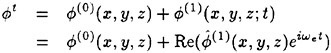
(8)
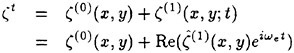
(9)
Correspondingly the symbol ^ is used for the complex amplitudes of all other first-order quantities, such as motions, forces, pressures, etc.
The superposition principle can be used within a linearized theory. Therefore the radiation problems for all 6 degrees of freedom of the rigid-body motions and the diffraction problem can be solved separately. The total solution is a linear combination of the solutions for each independent problem.
The harmonic potential ![]() is divided into the potential of the incident wave
is divided into the potential of the incident wave ![]() the diffraction potential
the diffraction potential ![]() and 6 radiation potentials:
and 6 radiation potentials:
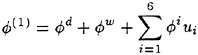
(10)
It is convenient to divide ![]() and
and ![]() into symmetrical and antisymmetrical parts to take advantage of the (usual) geometrical symmetry:
into symmetrical and antisymmetrical parts to take advantage of the (usual) geometrical symmetry:
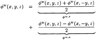
(11)
(12)
The linearized potential of the incident wave on water of infinite depth is expressed in the inertial system:
(13)
(14)
![]() is the frequency of the incident wave, ωe=|ω−kU cοs μ| the frequency of encounter, k is the wave number. The derivation of the expression for
is the frequency of the incident wave, ωe=|ω−kU cοs μ| the frequency of encounter, k is the wave number. The derivation of the expression for ![]() assumes a linearization around z=0. The same formula will be used now in the seakeeping computations, although the average boundary is at the steady wave elevation, i.e. different near the ship. This may be an inconsistency, but I believe that the introduced errors are small.
assumes a linearization around z=0. The same formula will be used now in the seakeeping computations, although the average boundary is at the steady wave elevation, i.e. different near the ship. This may be an inconsistency, but I believe that the introduced errors are small.
The steady flow contributions are determined in a ‘fully nonlinear’ wave-resistance code employing higher-order panels, [12]. The second derivatives of the potential in x-direction are limited to the maximum value at 80% of the ship length in the aft-body to avoid unrealistically high values at the stern reflecting to some extent the effect of viscosity in reality. This yields the steady dynamic trim and sinkage, the steady wave elevation and the first and second derivatives of ![]() . It is convenient to introduce the following abbreviations for steady flow contributions:
. It is convenient to introduce the following abbreviations for steady flow contributions:
(15)
(16)
(17)
3. Problem formulation
Consider a ship moving with mean speed U in a harmonic wave of small amplitude in an ideal fluid. The fundamental field equation is then Laplace’s equation. This equation has to be fulfilled in the whole fluid domain. In addition, we formulate the following boundary conditions:
-
Water does not penetrate the ship hull. (Hull condition)
-
Water does not penetrate the free water surface. (Kinematic free-surface condition)
-
There is atmospheric pressure on the free surface. (Dynamic free-surface condition)
-
There is undisturbed flow far away from the ship. (Decay condition)
-
Waves created by the ship propagate away from the ship. Depending on the frequency of these waves and the speed of the ship, waves may be limited to a sector, namely propagating only downstream. (Radiation condition)
-
At the trailing edge of the ship (stern), the pressures are equal on both sides. (Kutta condition)
-
Waves created by the ship must leave an artificial boundary of the computational domain without reflection. (Open-boundary condition)
-
The forces on the ship result in periodic motions. (Equilibrium)
We assume that the time-averaged added resistance is compensated by increased propulsion forces, i.e. the average speed remains constant.
Conditions [e], [f] and [g] deserve a more detailed discussion. The presented method is so far limited to cases with τ=ωeU/g>0.25. ωe is the encounter frequency, g=9.81 m/s2. Techniques to extend Rankine panel methods to arbitrary τ, [2], require considerably higher computational effort and shall be subject to future investigations. For the selected test cases here, as for most ships, a restriction to τ>0.25 excludes only following waves, Fig. 1. For
τ>0.25, the radiation condition is analogous to the steady wave resistance problem on shallow water for undercritical depth Froude numbers. The numerical ‘shifting’ technique developed originally for the steady wave-resistance case can be adapted without problem to the time-harmonic problem, [13], and fulfills also automatically the open-boundary condition [f].
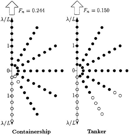
Fig. 1: τ>0.25 (●) and τ<0.25 (○) for two ships
The ship (especially including the rudder) can be considered as a vertical foil of extremely short span. For a steady yaw angle, i.e. a typical manoeuvring application, one would certainly enforce a Kutta condition in a potential flow computation. However, for the corresponding periodic motion in seakeeping, the Kutta condition is rarely even mentioned for 3-d methods. Wu [14] includes the Kutta condition to compute the radiation problem for an oscillating surface-piercing plate at forward speed using a Green function method. Zou [15] solves the same problem using a Rankine panel method. The only application to a ship at forward speed is an extended abstract by Zou [16]. However, Zou solves only the radiation problem and neglects the steady disturbance potential. For the related problem of fluttering vibrations of airfoils in aerospace engineering, enforcing a Kutta condition appears to be standard procedure. It is unclear if omitting the Kutta condition is based on some physical insight about the negligible effects or oversight. It is of no importance as long as the applications are limited to head or following waves, i.e. the most frequent test cases. But of course, for practical requirements a method must be applicable for all wave directions.
The boundary conditions are linearised with respect to h (and all other related time-harmonic quantities). Detailed derivations of the free-surface and hull conditions can be found in [4].
At the average free surface (z=ζ(0)) a combination of dynamic and kinematic free-surface conditions gives:
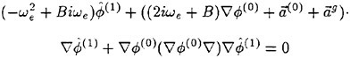
(18)
This equation corresponds to eq. 3–23 of Newman [17].
Let the ship hull be defined in the ship-fixed system by ![]() . Then after introducing the m-terms
. Then after introducing the m-terms ![]() the boundary condition at
the boundary condition at ![]() becomes:
becomes:
(19)
This equation corresponds to eq. 3–30 of Newman [17].
The unsteady pressure p(1) is decomposed into contributions from the incident wave, diffraction, and radiation:
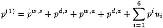
(20)
where each unsteady pressure component on the r.h.s. is computed in the linearised form:
(21)
The Kutta condition requires that at the trailing edge the pressures are equal on both sides. This requires zero complex amplitudes for the antisymmetric pressure:
(22)
i=1, 3 and 5 for the three antisymmetric radiation modes and i=d for the antisymmetric diffraction part.
The unknown diffraction and unit motion radiation potentials can be determined independently. Rankine elements fulfill automatically again Laplace’s equation and the decay condition. The hull is discretized with special first-order panels evaluated by numerical integration. Desingularized Rankine point singularity clusters are used on a layer above
the free surface. Details of these elements are described in [4], but the method should work with any first-order elements, e.g. regular Hess&Smith panels. Collocation points are located only on starboard. Mirror images of all Rankine elements account for the port side.
For the diffraction problem, all ui and αi are set to zero. For a radiation problem, the relevant motion amplitude is set to 1 and all other motion amplitudes, ![]() and
and ![]() to zero. Then free-surface condition (18) and the hull condition (19) are fulfilled in a collocation scheme. For the antisymmetric problems, also the Kutta condition (22) is fulfilled at the last column of collocation points at the ship stern. A corresponding number of Thiart elements (semi-infinite dipole strips on the plane y=0, see Appendix) is used. The dipole strips start amidships and have the same height as the corresponding last panel on the stern. Radiation and open-boundary condition are enforced by ‘staggering’ the Rankine sources for the free surface relative to the collocation points by one typical grid spacing downstream, [13]. (This technique is only applicable for τ>0.25; other cases cannot be covered so far.) The collocation scheme forms eight systems of linear equations in the unknown element strengths. The four symmetrical (likewise the four antisymmetrical) systems of equations share the same coefficient matrix with only the r.h.s. being different. All four cases are solved simultaneously using Gauss elimination. After solving the systems of equations, only the motions ui remain to be determined.
to zero. Then free-surface condition (18) and the hull condition (19) are fulfilled in a collocation scheme. For the antisymmetric problems, also the Kutta condition (22) is fulfilled at the last column of collocation points at the ship stern. A corresponding number of Thiart elements (semi-infinite dipole strips on the plane y=0, see Appendix) is used. The dipole strips start amidships and have the same height as the corresponding last panel on the stern. Radiation and open-boundary condition are enforced by ‘staggering’ the Rankine sources for the free surface relative to the collocation points by one typical grid spacing downstream, [13]. (This technique is only applicable for τ>0.25; other cases cannot be covered so far.) The collocation scheme forms eight systems of linear equations in the unknown element strengths. The four symmetrical (likewise the four antisymmetrical) systems of equations share the same coefficient matrix with only the r.h.s. being different. All four cases are solved simultaneously using Gauss elimination. After solving the systems of equations, only the motions ui remain to be determined.
The expressions to determine the motions are derived in principle from ‘force=mass · acceleration’ to:
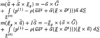
(23)
![]() is the ship’s weight, m the displacement mass,
is the ship’s weight, m the displacement mass, ![]() the center of gravity, I the matrix of mass inertia moments with respect to the origin of the ship-fixed system. Mass distribution symmetrical in y is assumed:
the center of gravity, I the matrix of mass inertia moments with respect to the origin of the ship-fixed system. Mass distribution symmetrical in y is assumed:
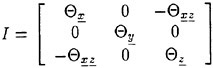
(24)
Θx, etc. are the moments of inertia and the centrifugal moments with respect to the origin of the body-fixed Oxyz-system:
(25)
The radii of inertia are defined as ![]() etc.
etc.
Thrust and resistance forces acting on the ship are affected by the motions. One could include thrust and resistance vectors similar to the weight vector ![]() to account for all motions. However, the main effect comes from surge motions in long waves and this allows a simpler treatment. Surge motions change the longitudinal velocity of the ship. Correspondingly changed resistance and propulsion characteristics of the ship will damp surge motions especially for long waves. Also the local orbital velocity of the waves may have some influence. If these effects are neglected, surge motions are overestimated by the computation. The thrust Th depends the instantaneous speed of advance of the propeller υa:
to account for all motions. However, the main effect comes from surge motions in long waves and this allows a simpler treatment. Surge motions change the longitudinal velocity of the ship. Correspondingly changed resistance and propulsion characteristics of the ship will damp surge motions especially for long waves. Also the local orbital velocity of the waves may have some influence. If these effects are neglected, surge motions are overestimated by the computation. The thrust Th depends the instantaneous speed of advance of the propeller υa:
(26)
υa,0=(1−w)U is the speed of advance of the propeller at steady speed U, w is the Taylor wake fraction, and the location of the propeller ![]() . For long waves, the contribution of the incident wave will dominate and the diffraction part may be neglected, [18]. Th is developed in a linear Taylor expansion around υa,0:
. For long waves, the contribution of the incident wave will dominate and the diffraction part may be neglected, [18]. Th is developed in a linear Taylor expansion around υa,0:
(27)
The calm-water resistance R at an instantaneous speed is similarly developed in a Taylor expansion around U:
(28)
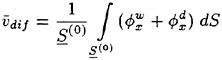
(29)
![]() approximates the influence of the orbital velocity averaging over the wetted surface of the ship. For short waves, this will lead automatically to negligible values, leaving contributions only for long waves. Thrust and resistance at calm-water speed cancel, yielding:
approximates the influence of the orbital velocity averaging over the wetted surface of the ship. For short waves, this will lead automatically to negligible values, leaving contributions only for long waves. Thrust and resistance at calm-water speed cancel, yielding:
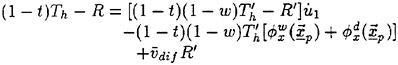
(30)
This expression is added as correction on the r.h.s. of the first component of vector eq. (23). The ![]() term can be interpreted as surge damping, the remaining terms contribute to the exciting surge force.
term can be interpreted as surge damping, the remaining terms contribute to the exciting surge force. ![]() R′, thrust deduction fraction t and w are taken
R′, thrust deduction fraction t and w are taken
from model tests or—if these are not available—approximated by empirical formulas. Numerical tests showed, however, that the the last two terms in (30) affect the results by less than 1% and may therefore be omitted, [11].
Surge-corrected Eqs. (23) yield a system of linear equations for ui (i=1, …, 6) which is quickly solved by Gauss elimination.
Following a similar approach as for the first-order forces, a formula for the added resistance can be derived that uses only quantities computed so far:
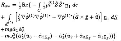
(31)
The asterisk indicates a conjugate complex. The formula assumes wall-sided hulls in the steady waterline. C is the vertical projection of the steady wave profile. This modified waterline contour accounts also for steady trim and sinkage and differs usually from the still waterline contour. Z is the first-order difference between average (steady) and instanteneous wave profile on the hull:
(32)
The term ∇p(1) involves again second derivatives of the potential on the hull:
(33)
However, as long as there is no panel element that computes both potential and second derivatives, the second derivatives of the harmonic potentials are neglected (‘desperation rather than physical insight’). It will have to be subject to further numerical investigations whether this introduces really any significant errors.
The integrals in Eqs. (31) (like the integrals in (23)) are evaluated numerically over the starboard half only and multiplied by 2 for symmetrical/symmetrical and antisymmetrical/antisymmetrical pressure-normal combinations only. (Antisymmetrical/symmetrical combinations yield zero contributions.)
4. Applications
4.1. Series-60 in head waves
The Series-60 with CB=0.60, Table I, was discretized with 594 elements. The steady problem was solved for Fn=0.2 with 1422 elements on the free surface. Trim and sinkage agreed well with experiments. The same hull grid was used for the seakeeping computations. For each investigated wave length, a new structured grid was generated on the free surface and the results of the steady computation were interpolated in this grid. The grids had between 1400 and 1700 elements.
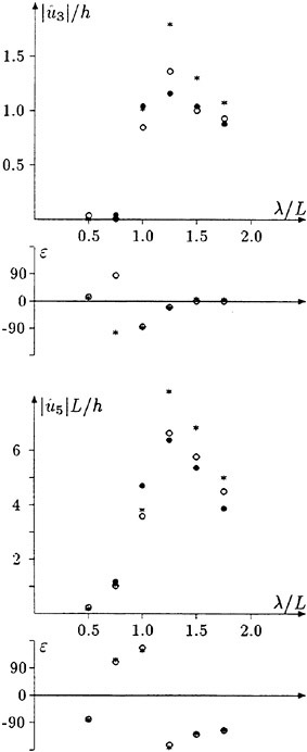
Fig. 2: RAOs for Series 60, μ=180°, Fn=0.2,
● experiment,
○ 3-d RSM (‘fully 3-d’),
* 3-d RSM (uniform flow approximation)
Fig. 2 shows the RAOs for heave and pitch. For comparison, also results with the same grids are shown, when the classical approximation (uniform flow, no dynamic trim and sinkage) is used. The fully 3-d method agrees much better with experiments. The classical approximation leads to overprediction by some 20%.
Table I: Series-60 ship
|
CB |
0.6 |
|
Lpp |
121.92 m |
|
Β |
16.25 m |
|
Τ |
6.50 m |
|
m |
7726 t |
|
xg before Lpp/2 |
−1.8 m |
|
zg below CWL |
0.9 m |
|
kx/L |
0.055 |
|
ky/L |
0.25 |
|
kz/L |
0.23 |
|
kxz/L |
0.0 |
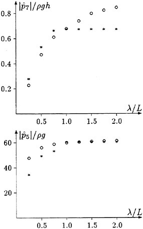
Fig. 3: Diffraction pressure and pressure due to unit pitch motion at a bow panel for Series 60, μ=180°, Fn=0.2, ○ 3-d RSM (‘fully 3-d’),
* 3-d RSM (uniform flow approximation)
Besides integral values like forces and motions, sometimes local pressures are of interest, especially in the bow region. Therefore, for a strip of panels in the forebody the computed pressures were compared between the fully 3-d method and the classical approximation for one wave length, [6]. For one point in the bow region (x/L=0.4753, y/B=0.00107, z/T=0.9488), Fig. 3 shows the diffraction pressure (without the contribution of the incident wave) and the radiation pressure due to unit pitch motion for various wave lengths. For the diffraction pressure, the differences increase for longer wave lengths. For the radiation pressure due to pitch unit motion, significant differences occur only for shorter waves. The diffraction pressure dominates for short waves (motions almost zero), but the radiation pressures for long waves. This explains probably why the motions are computed well for long and short waves. The large relative errors occur here in unimportant pressure parts. However, for medium wave lengths—where the maxima of the motions occur—errors apparently superpose to such an extent that the influence of the steady flow becomes considerable for the motion prediction.
4.2. S-175 in head waves and oblique waves
The S-175 containership, Table II, was computed for the design condition with Fn=0.275. The hull was discretized by 631 elements, [11]. For the nonlinear wave-resistance problem, the free-surface structured grid used 1430 elements. Sinkage was predicted at 0.0025 Lpp and trim 0.00045 aft.
Table II: S-175 containership data
|
CB |
0.5716 |
|
Lpp |
175.00 m |
|
B |
25.40 m |
|
T |
9.50 m |
|
m |
24742 t |
|
xg before Lpp/2 |
2.48 m |
|
zg below CWL |
−0.02 m |
|
kx/L |
0.0476 |
|
ky/L |
0.24 |
|
kz/L |
0.24 |
|
kxz/L |
0.0 |
The same discretized hull model was used for the seakeeping computations. Grids on the free surface had then in each case about 1300 elements. Fig. 4 shows the response amplitude operators for motions for head waves. The results of the presented panel method agree generally well with experiments for all motions and all frequencies. Only for higher frequencies, experimental and computed phases differ sometimes considerably. However, in these cases the absolute values are almost zero and in this case the phase is insignificant. The surge motions for low frequencies are computed somewhat higher than measured. The reason is unclear, but could lie in nonlinear effects or margins of errors in the experiments. For comparison, the classical approximation yields again overpredictions for heave and pitch motions of about 20% for medium wave lengths. There are several steady free-surface effects which in sum create the above differences. One of these effects can be incorporated relatively simply in all seakeeping methods: dynamic trim and sinkage. The dynamic trim and sinkage may be computed by any Rankine panel method or esti-
mated by simpler methods. Then for the resulting geometry a Green function method grid or a strip method grid may be created. To illustrate the influence of just the effect of trim and sinkage, the computations were repeated with trim and sinkage suppressed in the steady computations. The results are marked by + in Fig. 4. The influence on heave is negligible in this case. However, for pitch in medium to long waves, about half of the discrepancy between the results considering all forward-speed effects and the classical approximation apparently can be contributed to not capturing trim and sinkage.
Computations for oblique waves were compared to experiments for μ=120°, (Fig. 5), μ=60°, (Fig. 6). Results for heave and pitch agree well with experiments.
For μ=120° the Kutta condition has only significant effects in the region where resonance occurs. Here the Kutta condition simulates to some extent the effect of viscous damping and reduces drastically (by factors between 2 and 4) the antisymmetric motions. However, additional viscous effects (those that would be apparent also at zero speed) reduce for roll in reality the motions even more. For yaw and sway, no experimental data are here available, but I expect that autopilots in experiments will also prevent the large predicted motion amplitudes of the computations.
For μ=60° some short-comings of the present method become apparent. Yaw is predicted with good accuracy over most of the range of frequencies, but for low frequencies (long waves) the computations overpredict motions strongly, even if a Kutta condition is enforced. I suspect that this is due to an autopilot used in experiments which restores motions for low frequencies. But this assumption requires further investigation. Roll motions show only satisfactory agreement between computations and experiments. Sway shows strong scatter of results. Apparently the Kutta condition makes things worse here.
The results do not demonstrate a conclusive improvement due to the Kutta condition. The improvements for the narrow region of resonance are drastic, but ad hoc solutions limiting the response amplitude operators to maximum values taking from experiments for similar ships may work almost as well in practice, while being a lot simpler. Sway motions for low encounter frequencies (in following oblique waves) require special treatment. This will have to be subject to further research.
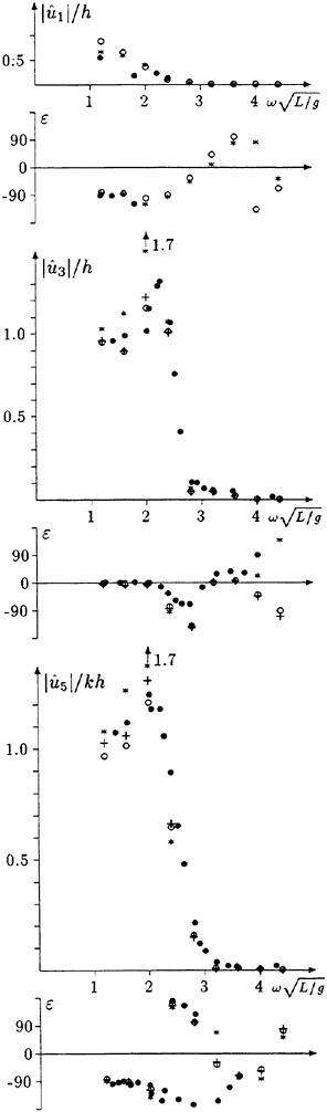
Fig. 4: RAOs for S-175, μ=180°, Fn=0.275; ● experiment, ○ RSM (‘fully 3-d’), * RSM (uniform flow approximation), + RSM (no trim and sinkage)
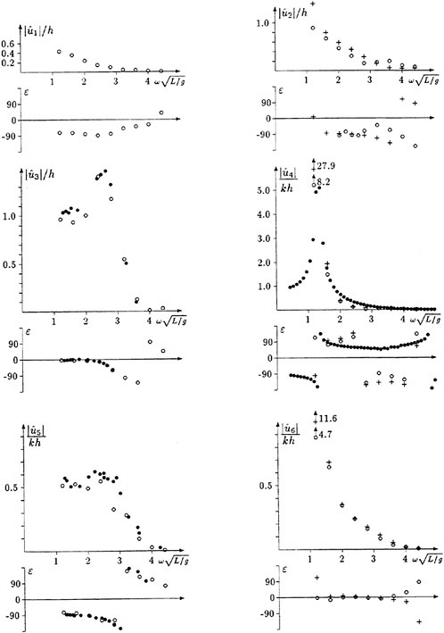
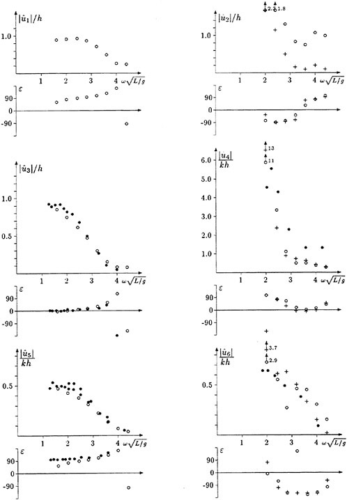
5. Conclusion
The ‘fully 3-d’ Rankine panel method to compute seakeeping of ships allows to investigate numerically the importance of capturing certain forward-speed effects, respectively to demonstrate that effects may indeed be neglected. I draw the following conclusions from the analysis of results obtained so far:
-
The effect of the steady flow is significant for motions. The classical approximation of uniform flow and calm-water sea and ship position introduces differences of about 20% for heave and pitch motions near the maxima of the motions.
-
Classical methods like strip methods or Green-function methods could relatively easily capture dynamic trim and sinkage and the dynamic wave profile. This should be done for high Froude numbers.
-
The Kutta condition failed to improve consistently results. Ad-hoc, semi-empirical corrections may rather be taken.
-
The surge correction proposed is easy to implement. However, only the first term is really significant.
-
The method requires considerable additional work to be become a practical alternative to existing seakeeping methods, foremost an extension to low τ values. But also further corrections for antisymmetric degrees of freedom, validation for full hulls, multihulls, transom stern ships, etc. are required.
-
The formula for added resistance has not yet been validated against experiments.
References
1. Fujii, H. and Takahashi, T., “Experimental study on the resistance increase of a ship in regular oblique waves,” 14th Int. Towing Tank Conf., 1975, pp. 351–360
2. Bertram, V. and Yasukawa, H., “Rankine source methods for seakeeping problems,” Jahrbuch der Schiffbautechnischen Gesellschaft, Springer, 1996, pp. 411–425
3. Hughes, M., “3-d Rankine panel computations for a ship in head waves”, 12th WWWFB, Hamburg, 1996
4. Bertram, V., “A 3-d Rankine panel method to compute added resistance of ships,” IfS Report 566, 1996, Univ. Hamburg
5. Kring, D.C., Huang, Y.F., Sclavounos, P.D., Vada, T. and Braathen, A., “Nonlinear ship motions and wave induced loads by a Rankine panel method,” 21th Symp. Naval Hydrodyn., Trondheim, 1996. pp. 45–63
6. Bertram, V., “Vergleich verschiedener 3D-Verfahren zur Berechnung des Seeverhaltens von Schiffen,” Jahrbuch der Schiffbautechnischen Gesellschaft, Springer, 1997
7. Bunnik, T. and Hermans, A., “A time-domain algorithm for motions of high speed vessels using a new free surface condition”, 13th WWWFB, Carry-le-Rouet, 1997, pp. 19–24
8. Iwashita, H. and Bertram, V., “Numerical study on the influence of the steady flow field in seakeeping,” 13th WWWFB, Carry-le-Rouet, 1997, pp. 119–122
9. Kring, D.C., Mantzaris, D.A., Tcheou, G.B. and Sclavounos, P.D., “A time-domain seakeeping simulation for fast ships,” FAST’97, Sydney, 1997. pp. 455–461
10. Van’t Veer, A.P., “Analysis of motions and loads on a catamaran vessel in waves,” FAST’97, Sydney, 1997, pp. 439–446
11. Bertram, V. and Thiart, G., “Fully three-dimensional ship seakeeping computations with a surge-corrected Rankine panel method,” to appear in J. Marine Science and Technology, 1998
12. Hughes, M. and Bertram, V., “A higher-order panel method for steady 3-d free-surface flows,” IfS Report 558, 1995, Univ. Hamburg
13. Bertram, V., “Fulfilling open-boundary and radiation condition in free-surface problems using Rankine sources”, Schiffstechnik 37/2, 1990, pp. 47–52
14. Wu, G.X., “Wave radiation by an oscillating surface-piercing plate at forward speed”, Int. Shipbuilding Progr. 41, 1994, pp. 179–190
15. Zou, Z.J., “A 3-d numerical solution for a surface-piercing plate oscillating at forward speed,” 10th WWWFB, 1995, Oxford
16. Zou, Z.J., “A 3-d panel method for the radiation problem with forward speed”, 9th WWWFB, 1994, Kuju
17. Newman, J.Ν., “The theory of ship motions,” Advances in Applied Mechanics 18, 1978, pp. 222–283
18. Zhou, Y., “Bestimmung der im Seegang zusätzlich erforderlichen Antriebsleistung von Schiffen,” IfS Report 490, 1989, Univ. Hamburg
19. Gerritsma, J., “Shipmotions in longitudinal waves,” 1960, ISP 7/66, pp. 49–71
20. Gerritsma, J. and Beukelman, W., “Analysis of the modified strip theory for the calculation of ship motions and wave bending moments,” 1967, ISP 14/156, pp. 319–337
21. Söding, H., “Springing of ships,” ESS-Report 7, 1975, Univ. of Hannover
Appendix: Velocity Potential for a Rectangular Vortex Panel with Harmonically Oscillating Strength
This element was developed by Dr Gerhart Thiart of Stellenbosch University.
The oscillating ship creates a vorticity. The problem is similar to that of an oscillating airfoil. The circulation is assumed constant within the ship. Behind the ship, vorticity is shed downstreams with ship speed U. Then:
(34)
γ is the vortex density, i.e. the strength distribution for a continuous vortex sheet. The following distribution fulfills condition (34) for x≤xα:
(35)
![]() is the vorticity density at the trailing edge xa (stern of the ship). We continue the vortex sheet inside the ship at the symmetry plane y=0, assuming like [16] a constant vorticity density. This yields for xa≤x≤xf:
is the vorticity density at the trailing edge xa (stern of the ship). We continue the vortex sheet inside the ship at the symmetry plane y=0, assuming like [16] a constant vorticity density. This yields for xa≤x≤xf:
(36)
xf is the leading edge (forward stem of the ship). This vorticity density is spatially constant within the ship.
A vortex distribution is equivalent to a dipole distribution if the vortex density γ and the dipole density m are coupled by:
(37)
The potential of an equivalent semi-infinite strip of dipoles is then obtained by integration. This potential is given (except for a so far arbitrary ‘strength’ constant) by:
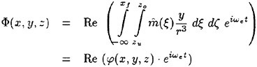
(38)
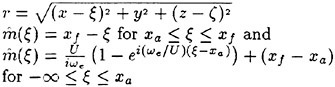
It is convenient to write φ as:
(39)
(40)
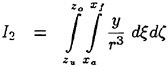
(41)
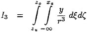
(42)
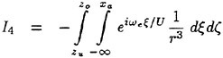
(43)
(44)
(45)
(46)
The velocity components and higher derivatives are then derived by differentiation of Φ, which can be reduced to differentiation of φ:
(47)
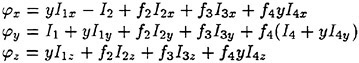
(48)
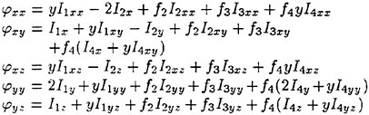
(49)
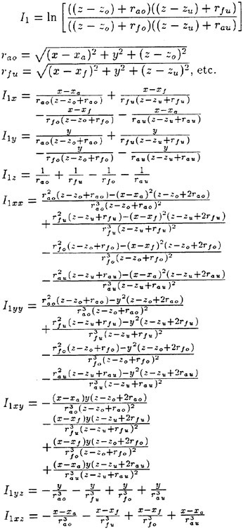
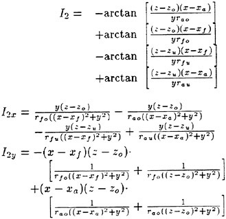
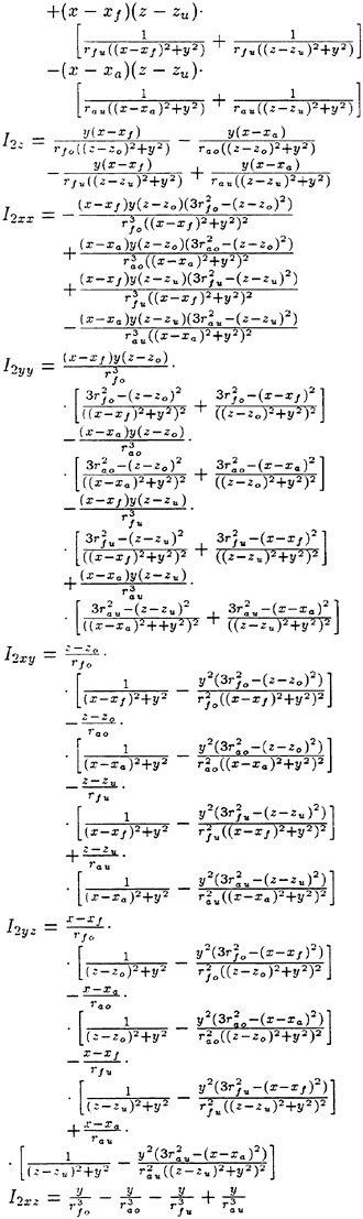
The integral I3 and its derivatives are:
(52)
The integral I4 and its derivatives are:
(53)
The integral with respect to ξ in the expressions for I4 and its derivatives are evaluated numerically following the modified Simpson’s method of [21]:
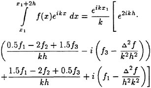
(54)
where f1=f(x1), f2=f(x1+h), f3=f(x1+2h), Δ2f=f1−2f2+f3.
The integration interval is truncated 0.1 · (xf−xa) up- and downstream of the the field point x. The wake “panel” is subdivided into a suitable number of “sub-panels” depending on the minimum distance of the field point to the wake.
DISCUSSION
Μ.Hughes
Analytical Methods, Inc., USA
I would like to congratulate the author on presenting an excellent paper describing a fully three-dimensional linearized seakeeping code based on Rankine panels. I was fortunate to have had the opportunity to work with the author in this area a few years ago while a post-doctoral research fellow at the IfS in Hamburg. At that time we developed a higher-order panel method for computing the steady flow contributions. Higher-order panels were used for that problem in order to compute the second derivatives of the velocity potential on the hull required for the m-terms. It is encouraging to see the progress that has been made since I have left, and I look forward to seeing comparisons for the added resistance predictions from this method.
It seems that the formulation of the Kutta condition requires that the condition be applied at the symmetry plane. As mentioned in the introduction to the paper, high-speed ships are one of the applications where the presented method is expected to have advantages over traditional strip theory methods. Such vessels are likely to be multi-hulled. Can the current procedure for satisfying the Kutta condition be extended to multi-hulled and other vessels where the Kutta condition must be satisfied away from the centerline? Also, have any convergence studies been performed to see if improved results may be obtained with a higher grid density on the hull?
AUTHOR’S REPLY
Thank you praising what really is still a fragment of academic interest. The extension of the method to multihulls (catamarans and trimarans) is the subject of our current research efforts in cooperation with INSEAN, Rome. The Kutta condition for the outriggers should then be applied also for the symmetrical modes. In essence, then equality of (linearized) total pressure both on the inside and outside of each outrigger would have to be enforced. This is no fundamental problem, but requires reprogramming and testing.
An Analysis of Second-Order Wave Forces on Floating Bodies by Using a Higher-Order Boundary Element Method
Y.-R.Choi, S.-Y.Hong (Korea Research Institute of Ships and Ocean Engineering, Korea), H.-S.Choi (Seoul National University, Korea)
Abstract
The wave diffraction and radiation problem is studied numerically by using a higher-order boundary element method. The convergence of the higher-order boundary element method is tested systematically for bodies of different shapes. For the second-order force, a particular attention is paid on the contribution of the second-order potential, following the line of Molin’s approach. For numerical evaluation, the free surface is divided into 3 subregions; inner, intermediate and outer ones. In the inner region, the integral is evaluated numerically by using higher-order boundary elements. In the intermediate region, semi-analytic form is constructed with the help of eigen functions. In the outer domain, the analytic solution is available. This subdivision scheme reduces the numerical burden remarkably.
1. Introduction
Recently nonlinear wave loads on ocean structures have been of central interest in marine hydrodynamics research. Although intensive efforts have been put in evaluating the wave load, this problem has not yet been completely solved. It is mainly due to the intrinsic complexity of nonlinear phenomena in the free surface, which demands a complicated formulation and an intensive computational effort.
The study on nonlinear wave loads was initiated by Havelock. He considered the second-order forces on a ship due to total reflection on one hand (1) and due to relative first-order motions on the other hand (2). Maruo (3) rigorously derived the second-order force in general form by using momentum theorems and Newman (4) extended it to second-order moment. These works are known as far-field method or momentum method. Pinkster computed the time mean steady drift force in Ref. (5), and also difference-frequency drift forces in Ref. (6) by directly integrating pressure over the body surface. The force due to the second-order potential was initially studied by Molin (7), whose work provided a clue for evaluating the sum-frequency excitation. After then, more general methods have been developed by Eatock Taylor & Chau (8) and Liu et al. (9), to name a few.
As a scheme for solving boundary-value problems, constant panel method (CPM) and higher-order boundary element method (HOBEM) can be utilized. The former is conventional after Hess and Smith (10). It assumes that the values of physical quantities and geometry on a panel are constant. Therefore it needs a huge amount of panels to obtain accurate numerical results. In contrast with CPM, HOBEM is based on the assumption that physical quantities and geometrical shape are continuously vary and they are regarded as the variables by using mathematical shape functions on each element. It is known that it provides more accurate results with less numerical calculation, compared with CPM. Liu, et al. (11) showed the efficiency of HOBEM in hydrodynamics. Boo (12) introduced discontinuous elements to HOBEM in the wave resistance problem and Hong (13) combined the spline scheme and HOBEM.
In this paper we tried to verify the efficiency of HOBEM, more systematically. Convergence tests for a smooth body and a sharp edged body are performed to the first- and second-order forces. And a scheme for removing irregular frequency is described.
In addition, the characteristics of the second-order force is briefly reviewed. And then an effective method for evaluating the force due to the second-order potential is derived, which reduces the computational effort significantly. As numerical examples, the second-order forces on a sphere and ISSC tension-leg platform are evaluated.
2. Formulation of Boundary-Value Problem
The fluid is assumed to be inviscid and incompressible, and the flow is irrational. The governing equation becomes the Laplace equation for the velocity potential.
(1)
In addition to this, following boundary and radiation conditions are imposed on boundary surfaces (see Fig. 1).
Free Surface Condition

(2)
Body Boundary Condition
(3)
Bottom Boundary Condition
(4)
Radiation Condition
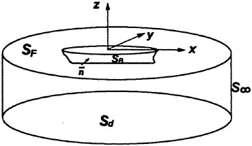
Fig. 1: Coordinate System
Based on the perturbation method for small amplitude waves, the velocity potential and other physical quantities are expanded with respect to the mean position of the body. Then the first-order boundary-value problem is well known, for example in Ref. (14). The first-order wave potential can be decomposed into incident, radiation and scattered parts.
(5)
(6)
The second-order boundary-value problem is complex due to nonlinear interaction terms in the free surface and body surface conditions as follow;
(7)
(8)
The right-hand side of eq. (7) consists of the products of first-order quantities like
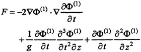
(9)
Its physical meaning is interpreted as imposing oscillatory pressures on the free surface with sum- and difference-frequencies of component waves. Eq. (8) looks similar to the first-order radiation potential problem except the second term in the right-hand side. This additional term is the correction part due to the first-order motion, which contains second-order derivatives of potential. A detail description is found in Ogilvie (15).
As shown in from eq. (7) to eq. (9), the second-order potential problem is too complicated to attack it directly. As an approximation, we decompose the potential into the incident, radiation and scattered parts, exactly the same as in the previous first-order problem (7).
(10)
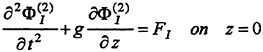
(11)
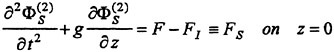
(12)
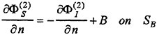
(13)
And the radiation part is expressed as the same manner as its first-order counterparts. Since we primarily concern with the second-order wave exciting force, we skip it.
3. Application of HOBEM
A particular characteristic of HOBEM compared to CPM is the introduction of shape functions. The geometric shape and physical variables are interpolated by shape functions in higher-order elements. Therefore boundary-value problem is solved more accurately by using a HOBEM (11).
3.1 8-node Boundary Element
In this paper, 8-node bi-quadratic elements are adapted. Fig. 2 illustrates this element and shape functions.
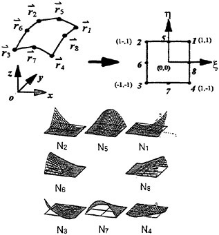
Fig. 2: 8-node bi-quadratic element and shape function
By using shape functions, the velocity potential and geometry are expressed as follows;
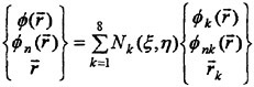
(14)
3.2 Integral Equation
The typical integral equation for velocity potential is well known. It contains dipole integral and solid angle, which cause numerical difficulties and require additional calculations. Eatock Taylor and Chau (8) derived an improved form of integral equation by adding an interior flow model, which removes dipole singularity and solid angle.
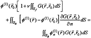
(15)
where,
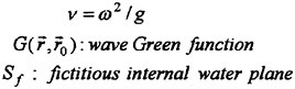
However, the wave Green function causes unfavorable interior resonant flow, known as irregular frequency problem. To prevent this difficulty, the condition for zero potential in the interior water plane is put into the eq. (15) (16). The resulting integral equation becomes
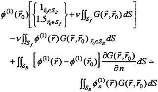
(16)
For the purpose of numerical evaluation, the body surface and interior water plane are discretized into higher-order elements. Then the integral equation turns to be algebraic equation.
(17)
In the above equation, NT is the number of nodes including that of interior surface. Detailed descriptions for influence matrix, Dji and Aji, are shown in Choi (17).
The source and dipole integrals on the singular element are performed with the help of polar-triangular transformation (11).
3.3 Derivatives by Using Higher-Order Element
The evaluation of the second-order force requires derivatives. In CPM, it is performed by differentiating given integral equation. However, its numerical work is awkward due to the increased strength of singularity on singular elements. On the contrary, it is simple in HOBEM, because the velocity potential and geometrical shape are expressed in terms of mathematical shape functions. Derivatives of them are also expressed in terms of the derivatives of the shape functions.
For first-order derivatives, the transformation of coordinates is to be
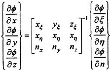
(18)
For second-order derivatives, 6 values of second-order derivatives must be known in the mapped coordinate system. But ![]() can not be defined. If the Laplace equation is satisfied on boundary surfaces, the unknown can be calculated. For example, transformed second-order derivatives are like below;
can not be defined. If the Laplace equation is satisfied on boundary surfaces, the unknown can be calculated. For example, transformed second-order derivatives are like below;
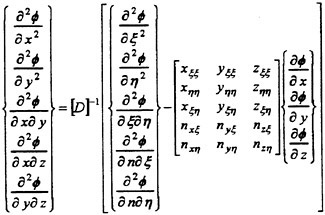
(19)
where,
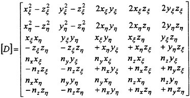
(20)
4. Second-Order Wave Forces
Nonlinear wave forces are attributed to the nonlinearity of the free surface and the body motion. To the second-order of wave amplitude, this effect is represented by mutual interaction of the first-order quantities. Thus characteristic frequency of the second-order force is either difference- or sum-frequency of component wave frequencies of ωk and ωl.
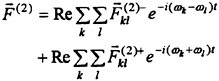
(21)
(22)
The difference part, denoted by Fkl(2)−, may cause large slowly-varying motions of a moored vessel, and the sum part, denoted by Fkl(2)+, may cause high-frequency vertical vibrations of a tension-leg platform, so called springing. In the light of physical origins, the second-order force can be divided into two parts; quadratic products of the first-order properties and the second-order potential. The former, denoted by Fqkl(2), was derived systematically by Pinkster (5), and it can be calculated by using the first-order solutions only. But the evaluation of the latter, denoted by Fpkl(2), is very difficult due to the complicated second-order potential.
Previous studies and experiments sofar clarify that the Fqkl(2)− part is dominant in the differnce-frequency components (18). However, in the sum-frequency component, the Fpkl(2)+ part can not be neglected in comparison with Fqkl(2)+. Recent studies on this force due to the second-order potential are activated in phase with the appearance of tension-leg platforms. The last component in eq. (22), Frkl(2)±, is the hydrostatic restoring force due to the second-order motions.
4.1 Second-Order Potential Force
The second-order potentials, which satisfy the Laplace equation and boundary conditions from eq. (11) to eq. (13), can be expressed as the sum of difference- and sum-frequency parts.
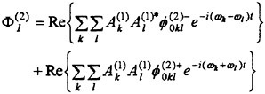
(23)
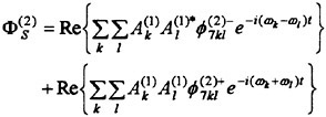
(24)
In the above equations, * denotes complex conjugate. The incident wave potential in eq. (23) is known by Bowers (19).
As stated previously, we concentrate herein on the second-order wave exciting force due to the incident and scattered waves. The formulation of the second-order excitation is quite similar for both differnce- and sum-frequency components. The wave exciting force is normalized by the square of wave amplitude to take
(25)
where the subscript j denotes the direction of the force and moment. The symmetry relation is well known so that one can evaluate it in the lower half region of the frequency the combination diagram.
(26)
To evaluate the force, the second-order scattered potential must be sought, as shown in eq. (12) and eq. (13). Molin (7) solved this problem by using the Haskind relation. His result contains the first-order quantities only.
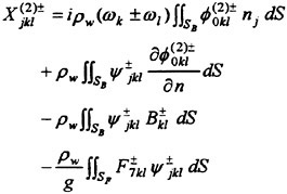
(27)
where F7kl± is the complex form of the free surface forcing term in eq. (12), corresponding to sum- and difference-frequencies. Auxiliary potential ψjkl± is exactly the same as the first-order radiation potential with sum- and difference-frequencies. The first and second terms in the right-hand side of eq. (27) are the contribution of incident waves and the third one comes from the first-order motions. These terms can be evaluated by using solutions of the first-order problem and the second-order incident waves. However, the last integral is to be performed over the entire free surface. Most previous researches on this topic have focussed on developing numerical schemes, in order to evaluate accurately over a finite region. This direct integration requires long computation time and huge computer memory. It was known that the convergence of the integral according to the size of region is rather poor (9). Another difficulty is that, as shown in eq. (8) and eq. (9), the kernel contains higher-order derivatives and accurate first-order quantities must be available. It can be tied over by using HOBEM.
To overcome the difficulty of integral over entire free surface, it is divided into 3 subregions; inner, intermediate and outer ones (See Fig. 3).
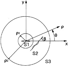
Fig. 3: Subdivision of Free Surface
4.2 Inner Region
In the inner region, the surface integral is evaluated accurately by using higher-order elements. This method requires less number of elements than CPM. The values of the potential in this region are calculated by using integral equation. Second-order
derivatives are evaluated by the scheme as explained previously, after some modifications.
4.3 Intermediate Region
In the intermediate region, all the integrands are expanded in terms of eigen functions in cylindrical coordinates.
(28)
En and Bem are eigen functions in the vertical and radial directions, which are expressed by hyperbolic functions and Bessel functions, respectively. kn are eigen values, called wave numbers. As shown in eq. (9) and eq. (27), the integrands consist of products of 3 first-order potentials. The integrals of the circumferential direction can be evaluated analytically with the help of the orthogonality of sinusoidal functions. The integrals in the radial direction are performed numerically. This semi-analytic approach saves numerical burden considerably. More detailed descriptions on eigen functions and coefficients are shown in Choi (17).
4.4 Outer Region
In the outer region, asymptotic expansions of integrands are utilized. After the integral is approximated in the circumferential direction by using the method of stationary phase, the integral from the radial distance ρ2 to infinity is carried out analytically. This yields to as follow;
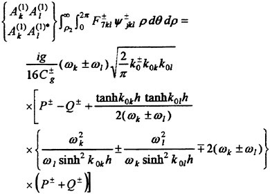
(29)
where
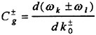
Ρ± and Q± are expressed in terms of Fresnel functions, which correspond to the stationary phase of β and β+π, respectively. Since the numerical domain can not cover the whole region, it serves as correction to numerical results. Its value oscillates rapidly and decays slowly as shown in Fig. 4. Therefore the convergence of the result as a function of the size of numerical region, S1 and S2, is poor. To obtain an accurate result, the contribution of the outer region should be considered.
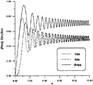
Fig. 4: Fresnel Functions
5. Numerical Results and Discussions
5.1 HOBEM vs. CPM
To demonstrate the advantage of HOBEM, a comparison study for HOBEM and CPM is made. For this purpose, hydrodynamic properties of a sphere and a rectangular barge are calculated.
■ Sphere
Since some analytic results are available, sphere is one of popular objects for validation study. To test the convergence, three different discretizations are adopted for CPM and HOBEM, respectively.
Heave added mass in deep water is shown in Fig. 5. Compared with the analytic result of Hulme (20), the convergence rate of HOBEM is faster than that of CPM. Hence, accurate results can be obtained with less number of elements by using HOBEM. Also, it can be seen that the scheme of eq. (16) guarantees
the successful removal of irregular frequencies in a wide frequency range.
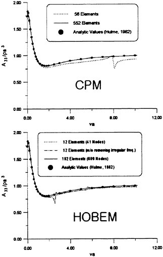
Fig. 5: Heave Added Mass of Floating Hemisphere
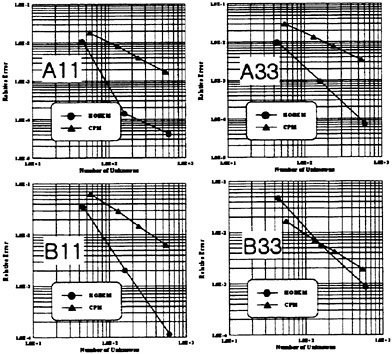
Fig. 6: Convergence diagram of Floating Hemisphere
A convergence diagram is represented in Fig. 6. In this figure, the number of unknowns means the number of elements for CPM and the number of nodes for HOBEM. The relative error is calculated by using analytic value at va=1.0, and the convergence rate is found as follow.
|
surge added mass |
∝ 1/N1.0 ∝ 1/N2.1 |
for CPM for HOBEM |
|
heave added mass |
∝ 1/N1.0 ∝ 1/N1.9 |
for CPM for HOBEM |
|
surge damping |
∝ 1/N1.0 ∝ 1/N2.2 |
for CPM for HOBEM |
|
heave damping |
∝ 1/N1.0 ∝ 1/N1.5 |
for CPM for HOBEM |
The convergence of HOBEM with quadratic-order is approximately double of CPM, except for heave damping. Therefore we can conclude that HOBEM is a very accurate and efficient scheme.
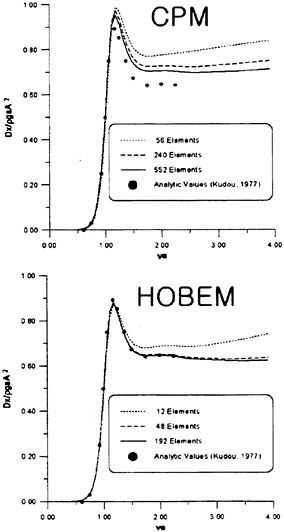
Fig. 7: Time Mean Surge Drift Force of Floating Hemisphere
The comparison is also earned out for the time mean drift force. The results are shown in Fig. 7, where analytic result of Kudoh (21) is included. Considering first-order quantities, the CPM gives the force overestimated and the convergence is very slow, especially in high frequency range. However, the accuracy and convergence of HOBEM is excellent. Only 48 elements are sufficient. To calculate the time mean drift force, first-order derivatives of the velocity potential should be evaluated. Hence, the derivative scheme, eq. (18), is highly recommended. It can be concluded that HOBEM is very useful for the evaluation of the second-order force.
■ Rectangular Barge
This geometry is chosen to understand the effect of shapes with sharp edges. The size of barge is 30 m(L)×22 m(B)×1.5 m(T), and displacement is 990 m3. It floats freely in water of depth 15 m. In order to test the convergence, four different discretizations are used for CPM and HOBEM, as shown in Fig. 8 and Fig. 9. Panel 4 and element 4 discretize the sharp edge densely.
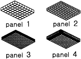
Fig. 8: Constant Panels (quadrant)
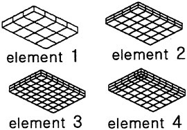
Fig. 9: Higher-Order Elements (quadrant)
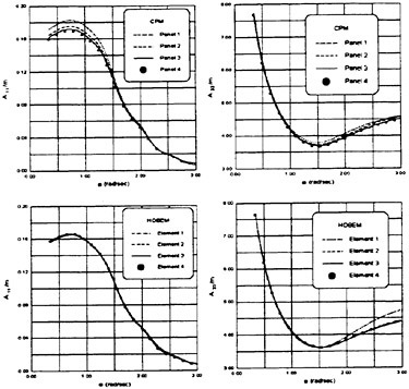
Fig. 10: Surge and Heave Added Mass of Barge
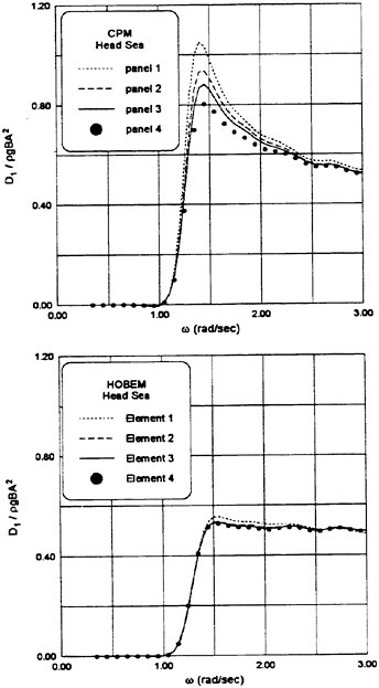
Fig. 11: Time Mean Surge Drift Force of Barge at Head Sea
It is seen from Fig. 10 that the convergence of HOBEM for hydrodynamic coefficients is faster than that of CPM. The added masses of surge and heave by CPM are larger than HOBEM. This is caused by neglecting solid angle at the edges. Since the solid angle is included in HOBEM, the effect of shape edge is taken into account more precisely.
In the case of the time mean drift force, noticeable differences are found between CPM and HOBEM. There exist apparent peaks in the CPM results and the peak magnitudes continue to decrease as the number of panels increases. In contrast, the convergence of the HOBEM results is very fast and the sharp peaks do not appear even for coarse discretizations. In the case of CPM, the result seems to be sensitive to the panel resolution near sharp edges. In the CPM results, the slightly negative drift is seen in the short range before the curve rises. This physically unacceptable result was reported in other works, especially for the drift of sharp edged bodies. However, the negative drift force is negligibly small in the result of HOBEM. It seems to be the effect of panel resolution near the sharp edge in CPM, also.
5.2 Second-Order Potential Force
The second-order potential force is known to be negligible in the difference-frequency excitation. Therefore only the sum-frequency excitation is considered. To verify the method developed herein, the second-order force on a sphere is calculated. And then, ISSC TLP is taken for a practical application.
■ Sphere
For sphere, the analytic values for the sum-frequency force are available in Ref. (22). They calculated it using the ring source integral equation method for water depth of 3×(radius of sphere).
Fig. 12 represents the discretization of the sphere and numerical free surface region, S1. The number of higher-order elements is 192 for the body and 256 for the free surface. The radius of S1 (=ρ1) is 3a.
In Fig. 13, surge and heave forces of double frequency are shown for a stationary sphere. The quadratic part of the force agrees with the analytic value. The evaluation of heave force is successful, also. However, some deviation in surge force is observed in the range of high frequencies. It seems to be caused by oscillations of auxiliary surge potential near the body surface in high frequency range. It can be seen that the second-order potential force makes a great contribution to the sum-frequency excitation.
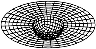
Fig. 12: Discretization of Sphere and Free Surface
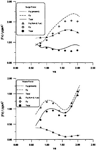
Fig. 13: Surge and Heave Force of Double Frequency on Stationary Sphere
In the case of a freely floating sphere, the results are shown in Fig. 14. In this figure, Fbb means the force due to the first-order motion as shown in eq. (27), which contains second-order derivatives. As shown in this figure, the second-order derivatives are performed accurately on the body surface. Hence, it can be concluded that the derivation scheme of eq. (19) and eq. (20) is very effective. The peak value near va=1 is induced by the heave motion at the natural frequency.
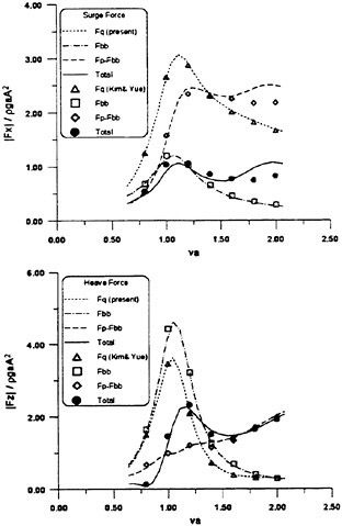
Fig. 14: Surge and Heave Force of Double Frequency on Freely Floating Sphere
In Fig. 15, the surge force caused by the free surface integral is illustrated. The results are compared with different size of inner and intermediate regions. The radius of the boundary between S2 and S3, is the same. It should be decided where the asymptotic expansion or the method of stationary phase are applied. In this paper, ρ2 is determined by the following equation.
In the above equation, k0 is the wave number of the longest wave among two component waves and auxiliary radiation wave. The value for small numerical region is the same as that for wider one. Therefore, it is demonstrated that the introduction of the intermediate region is successful. However, the results for a subregion (S1 or S2) are quite different dependent on the size. It implies that the integration is fluctuating largely according to the size of domain. The contribution from S3 is not negligible. It is mainly due to the interaction between the first-order incident wave and disturbed wave. Hence, one should take outer region integral into account.
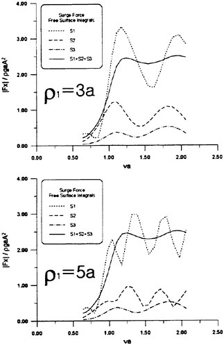
Fig. 15: Contribution of Free Surface Integrals on Freely Floating Sphere
■ ISSC TLP
As mentioned previously, high frequency forces like the sum-frequency excitation can excite the stiff vertical modes (heave, pitch and roll) of a tension-leg platform. For example, springing can cause the fatigue failure of tensioned tethers. Researches on the sum-frequency force are therefore focused on the application to the TLP. In this paper, the ISSC TLP is chosen as an example calculation. Its main dimensions are summarized as below;
Spacing between Column Centers (L): 86.25 m
Diameter of Column: 16.87 m
Breadth of Pontoon: 7.5 m
Height of Pontoons: 10.5 m
Draft: 35 m
Displacement: 54500 ton
Weight: 40500 ton
Water Depth: 450 m
More detail information is given in Eatock Taylor and Jefferys (23).
Fig. 16 represents the discretizations of the ISSC TLP and free surface region. The number of
higher-order elements is 140 and 512 for the body and free surface, respectively. The radius of S1 (=ρ1) is 90 m.
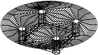
Fig. 16: Discretization of ISSC TLP and Free Surface
Double frequency heave and pitch excitations of the stationary TLP in head sea are shown in Fig. 17. The results are compared with the numerical results of Lee, et al. (24) and Liu, et al. (9) and also with the experimental result of Matsui, et al. (25). The qualitative trend of results is similar to each other. At high frequency, a good agreement with that of Lee, et al. (23) is found. They calculated with 4048 and 4928 constant panels for the body and free surface.
Fig. 18 shows the contributions of quadratic term and the second-order potential force in the pitch moment. It is seen that the contribution of quadratic term is small.
The results of the compliant TLP are represented in Fig. 19. They are very similar to the case of the stationary TLP. In the figure, Ff and Fb denote the component of free surface integral and body surface integral as given in eq. (27). The contribution of the free surface integral is dominant in the high frequency range. Hence, it should be noted that an accurate evaluation of the free surface integral is necessary to the sum-frequency excitation of TLP.
Fig. 20 shows the force due to the free surface integral and each subregion integral. The total value for small numerical region is the same as that with wide one. It means that an introduction of a wider intermediate region may save the numerical work for the inner region. In the pitch moment, the contribution from the outer region is remarkable.
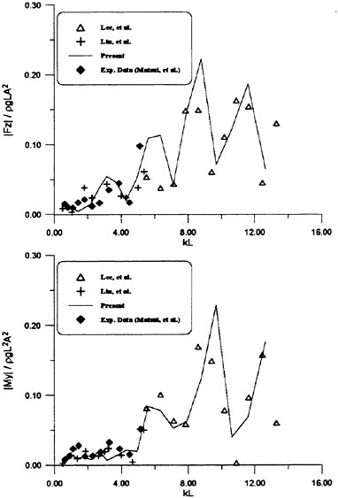
Fig. 17: Heave Force and Pitch Moment of Double Frequency on Stationary TLP
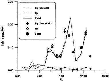
Fig. 18: The Components of Pitch Moment on Stationary TLP
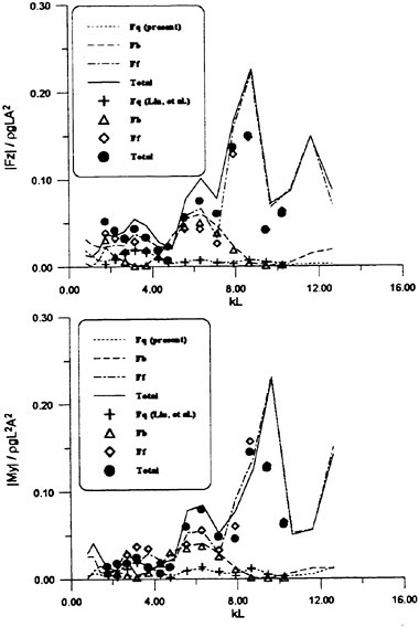
Fig. 19: Heave Force and Pitch Moment of Double Frequency on Compliant TLP
6. Conclusion
An accurate and efficient numerical scheme is constructed based on higher-order boundary elements. The convergence and accuracy are improved compared to the constant panel method. As shown in numerical examples, this scheme is particularly effective for the body with sharp edges.
The second-order potential force is formulated with the help of Molin’s approach. The difficulty of infinite free surface integral is overcome by introducing the intermediate and outer regions. It reduces the numerical burden remarkably. The wave force contribution from the far field is derived analytically in terms of Fresnel functions, which enhance the convergence of numerical results. Numerical examples shown herein clearly indicate the efficiency of the present method.
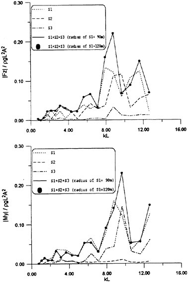
Fig. 20: Contribution of Free Surface Integrals on Compliant TLP
References
1. Havelock, Τ.Η., “The Pressure of Water Waves upon a Fixed Obstacle,” Proc. Royal Soc. London, Ser. A, Vol. 175, No. 963, 1940.
2. Havelock, T.H., “The Drifting Force on a Ship among Waves,” Phil. Magazine, Ser 7, Vol. 33, 1942.
3. Maruo, H., “The Drift of a Body Floating on Waves,” J. Ship Res., Vol. 4, No. 3, 1960.
4. Newman, J.N., “The Drift Force and Moment on Ships in Waves,” J. Ship Res., Vol. 11, 1967.
5. Pinkster, J.A., “Low Frequency Second Order Wave Forces on Vessels Moored at Sea,” Proc. 11th Symp. Naval Hydrodyn., 1976.
6. Pinkster. J.A., “Low Frequency Second Order Wave Exciting Forces on Floating Structures,” N.S.M.B., Pub. No. 650, 1980.
7. Molin, B., “Second Order Diffraction Loads upon Three-Dimensional Bodies,” Appl. Ocean Res., Vol. 1, 1979.
8. Eatock Taylor, R. and Chau, F.P., “Wave Diffraction—Some Development in Linear and Non-Linear Theory,” J. Offshore Mech. and Arctic Engng., No. 114, 1992.
9. Liu, Y.H., Kim, M.H. and Kim, C.H., “Double-Frequency Wave Loads on a Compliant TLP,” Proc. 3rd International Offshore and Polar Engng., 1993.
10. Hess, J.L. and Smith, A.M.O., “Calculation of Nonlifting Potential Flow about Arbitrary Three Dimensional Bodies,” J. Ship Res., Vol. 8, No. 3, 1964.
11. Liu, Y.H., Kim, C.H. and Lu, X.S., “Comparison of Higher-Order Boundary Element and Constant Panel Methods for Hydrodynamic Loadings,” J. Offshore and Polar Engng., Vol. 1, No. 1, 1990.
12. Boo, S.Y., “Application of Higher Order Boundary Element Method to Steady Ship Wave Problem and Time Domain Simulation of Nonlinear Gravity Waves,” Ph. D. dissertation, Texas A&M Univ., 1993.
13. Hong, S.Y., “Analysis of Steady and Unsteady Flow Around a Ship Using a Higher-Order Boundary Element Method,” Ph. D. Thesis, Seoul National Univ., 1994.
14. Newman, J.N., “Marine Hydrodynamics,” The ΜIT press, 1976.
15. Ogilvie, T.F., “Second-Order Hydrodynamic Effects on Ocean Platforms,” Proc. Intl. Workshop Ship and Platform Motions., 1983.
16. Hong, D.C., “On the Improved Green Integral Equation Applied to the Water Wave Radiation-Diffraction Problem,” J. Soc. of Naval Architects of Korea, Vol. 24, No. 1, 1987.
17. Choi, Y.R., “An Analysis of Second-Order Wave Forces by Using a Higher-Order Boundary Element Method,” Ph. D. Thesis, Seoul National Univ., 1997.
18. Choi. Y.R., Won, Y.S. and Choi, H.S., “The Motion Behavior of a Shuttle Tanker Connected to a Submerged Turret Loading System,” Proc. 4th International Offshore and Polar Engng., 1994.
19. Bowers, E.C., “Long Period Oscillations of Moored Ships Subject to Short Wave Seas,” Trans. R. Inst. Naval Archit., 1976.
20. Hulme, A., “The Wave Forces Acting on a Floating Hemisphere undergoing Forced Periodic Oscillations,” J. Fluid Mech., Vol. 121, 1982.
21. Kudoh, K., “The Drifting Force Acting on a Three-Dimensional Body in Waves,” J. of Soc. Nav. Arch. Japan, Vol. 141, 1977.
22. Kim, M.H. and Yue, D.K.P., “The Complete Second-Order Diffraction Solution for an Axisymmetric Body. Part 2. Bichromatic Incident Waves and Body Motions,” J. Fluid Mech., Vol. 211, 1990.
23. Eatock Taylor, R. and Jefferys, E.R., “Variability of Hydrodynamic Load Predictions for a Tension Leg Platform,” Ocean Engineering, Vol. 13, No. 5, 1986.
24. Lee, C.H., Newman, J.N., Kim, M.H. and Yue, D.K.P., “The Computation of Second-Order Wave Loads,” Proc. Offshore Mech. and Arctic Engng., 1991.
25. Matsui, T., Suzuki, T. and Sakoh, Y., “Second-Order Diffraction Forces on Floating Three-Dimensional Bodies in Regular Waves,” J. Offshore and Polar Engng., Vol. 2, No. 3, 1992.


