
Investigation of Waves Generated by Ships in Shallow Water
T.Jiang (Mercator University, Germany)
ABSTRACT
The shallow-water wave equations of Boussinesq type are used to simulate the ship waves at subcritical, transcritical, and supercritical speeds. An implicit difference method based on the Crank-Nicholson scheme is applied for the time and space discretization. The associated finite-difference equation system is then iteratively solved with controllable accuracy. To approximate the flow generated by a slender ship the technique of matched asymptotic expansions is used. Satisfactory agreement between calculations and model experiments is achieved for wave resistance, sinkage and trim as well as for wave profiles in the tank.
INTRODUCTION
Shallow-water ship-waves are characterized both by their dispersive nature as well as by their nonlinear nature. A ship moving in a shallow-water channel can shed so-called solitary waves when its speed is near the critical speed defined by depth Froude number Fnh=1.0. These solitary waves travel a bit faster in front of the ship and cause ship oscillations in the vertical plane. The wave pattern is thus unsteady relative to the ship. These nonlinear and unsteady phenomena were repeatedly observed in shallow-water towing tanks, e.g., Thews and Landweber (1935), Helm (1940), and Graff et al. (1964). In the theoretical investigation of ship waves at a near-critical speed in a channel considerable success has been recently achieved, e.g., Choi and Mei (1989) and Chen and Sharma (1995). The basic tool of these theoretical analyses is the technique of matched asymptotic expansions where the potential flow in the far field is approximated by a Kadomtsev-Petviashvili (KP) type of equation from the shallow-water wave-theory and the potential flow in the near field by using the slender-body theory. For practical application, this approximation technique has been refined by Chen and Sharma (1995) by using a modified KP equation, being valid in a broad range of speeds, and by improving the slender-body theory, considering the effects of longitudinal perturbation velocity and the dynamic submerged cross-section area. Satisfactory agreement between calculated and measured values of resistance and squat can be obtained, see Jiang et al. (1995) for a study of a catamaran passenger ferry in a shallow-water channel.
However, there is a fundamental restriction of the KP equation, namely, it is not valid for truly unsteady cases caused, for example, by the hydrodynamic interactions between passing ships, by the geographical changes of water bottom, by the wave-ship interactions near the coast, and so on. A theoretical approach for these unsteady cases is to solve the more general shallow-water wave equations of Boussinesq type, which are extensively used to simulate the one- and two-dimensional propagation of the nonlinear waves near a coast, e.g., Peregrine (1967), Madsen and Mei (1967), Madsen et al. (1991), Schröter (1995). In studying the shallow-water waves generated by a one-dimensional pressure distribution, the Boussinesq equations were applied by Wu and Wu (1982) and the Green-Naghdi equations by Ertekin et al. (1984), which are essentially of Boussinesq type and have been extended by Ertekin et al. (1986) to a two-dimensional pressure distribution moving in a narrow channel. In studying the shallow-water waves generated by a two-dimensional pressure distribution at transcritical speeds the Boussinesq equations were used by Pedersen (1988), where the pressure disturbance has been also approximated by an equivalent line-source distribution corresponding to the representation of the slender body in Mei and Choi (1987).
The present study focuses on the numerical implementation of the Boussinesq equations. The classical Boussinesq equations combine the nonlinear and dispersive effects of shallow-water waves so that waves with finite amplitude, such as solitary waves,
can propagate with unchanged shape. They should be valid for transcritical and supercritical speeds. In the subcritical speed range, not all wave components are long enough compared to the water depth. Therefore, the classical Boussinesq equations have to be modified. One established method for this is to improve the dispersion relation of the linearized Boussinesq equations by comparison with the linear wave theory. It can be theoretically shown that the modified Boussinesq equations used in the present study are valid for a ratio of wave length to water depth down to a value of 2, practically in the deep-water range. However, due to the influence of the high-oder terms the rapid upwind and high-resolution schemes for the Airy shallow-water wave equations, implemented by Jiang (1996), can not be applied for the Boussinesq equations. A new slow, but numerically more stable, implicit scheme is implemented to solve the initial/boundary value problem governed by the modified Boussinesq equations. It contains:
-
Crank-Nicholson scheme for the time and space discretizations
-
Approximation of the state values for the nonlinear terms by means of Taylor expansion
-
Iterative solution of the linear algebraic equation system
-
Overrelaxation to accelerate the convergence process
-
Local and global filtering to suppress the numerical oscillations
The newly developed computer programs are used to simulate the wave generation by a Series 60 hull moving uniformly in a shallow water channel. A slender-body theory along with the technique of asymptotic expansions is applied to approximate the flow generated by the hull. Both calculated integral quantities, such as wave resistance, sinkage and trim, as well as field quantities, such as wave profiles in the tank, are compared with those from recent measurements in the Duisburg Shallow Water Tank.
PROBLEM FORMULATION
General Description
For describing the flow generated by a ship at a uniform speed of V in a shallow water of constant water depth ho, a Cartesian coordinate system Oxyz is used, see Fig. 1. The plane Oxy is on the quiet free surface with the axes x in the direction of ship motion. The center O is on the intersection line of the midship section and the longitudinal centerplane, rendering the involved problem symmetric to the plane Ozx. The axis z is positive upward. The ship is free to heave and pitch; the midpoint sinkage is designated by s (positive downward) and the pitch angle by θ (positive bow-down).
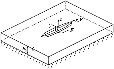
Fig. 1 Schematic of the problem and coordinate system
By virtue of this symmetry only the half fluid-domain on the starboard side of the ship is described in the following. On the assumption that the fluid is incompressible and inviscid, the irrotational flow generated by the moving ship can be described by a potential Φ governed by the Laplace equation,
(1)
in the whole fluid domain, and by the following boundary conditions: first, kinematic and dynamic conditions,
(2)
(3)
respectively, on the free surface z=ζ(x, y, t), where g is the acceleration due to gravity; second, no-flux condition,
(4)
on the hull-surface F(x, y, z, t)=0; third, no-flux condition,
(5)
on the water bottom z=−ho; fourth, no-flux condition,
(6)
on the centerplane y=0 as well as on the sidewall ![]() for the ship moving symmetrically in a straight horizontal rectangular channel of the width w; fifth, decay condition,
for the ship moving symmetrically in a straight horizontal rectangular channel of the width w; fifth, decay condition,
(7)
at infinity x → ±∞.
Shallow-Water Wave Approximation
Considering the wave generation by ships in a flow field with relatively small water depth, the well-established shallow-water wave-theory can be applied. The basic assumptions are that the waves are weakly nonlinear and long in comparison to water depth. The former implies that wave amplitude ζA is small compared with water depth ho, i.e., ε=ζA/ho≪O(1). The latter means that water depth is small compared with wave length λ. The combined result is a reasonable approximation of the potential Φ in terms of a locally depth-averaged potential φ defined as follows:
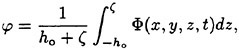
(8)
where ζ denotes the local wave elevation. Following standard shallow-water wave approximation (Taylor expansion in vertical direction) and disregarding all terms of order Ο[(μ=2πho/λ)4] or higher, the 3-D Laplace equation (1) and the water bottom condition (5) yield
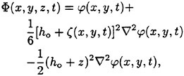
(9)
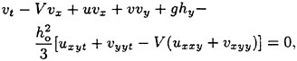
where the ∇-operator from now on takes its 2-D form, namely, ![]() . Substituting equation (9) into the kinematic and dynamic conditions (2) and (3) on the free surface, the Boussinesq equations are obtained for weakly nonlinear and moderately long waves of ε=μ2<1, see Mei (1989):
. Substituting equation (9) into the kinematic and dynamic conditions (2) and (3) on the free surface, the Boussinesq equations are obtained for weakly nonlinear and moderately long waves of ε=μ2<1, see Mei (1989):
(10)

(11)
(12)
where h=ho+ζ(x, y, t) is the local water depth and the depth-averaged horizontal velocity components are:
(13)
For the nonlinear long waves of μ → 0 and ε=O(1) the Airy equations are obtained:
(14)
(15)
(16)
which can be also directly derived from the 3-D Euler equations by assuming the pressure is proportional to the local submerged depth, i.e., p(x, y, z, t)=ρg[(ζ(x, y, t)+z], e.g., Wehausen and Laitone (1960).
The application of the above shallow-water wave equations to ship waves is some what restricted by the assumption of small ratio μ. Since all possible wave lengths are present in a ship wave pattern this assumption is not satisfied for wave components of small wave length, i.e., it violates the dispersion law of waves of small wave length. In recent years a considerable amount of research effort has been devoted to the improvement of the linear dispersion characteristics of Boussinesq equations, e.g., Witting (1984), Madsen et al. (1991), Nwogu (1993), Schröter (1995), and Dingemans (1997). The basic idea is to modify the Boussinesq equations by comparing their dispersion characteristics with those from the linear wave theory. One possibility is to add high-order linear terms to the dynamic equations (11) and (12). The modified Boussinesq equations read now:
(17)
(18)
(19)
with the coefficient CBQ needed to be specified. Its suitable value can be found by comparing the dispersion relation of the modified Boussinesq equations with that from the linear wave theory. For a stationary Kelvin ship-wave pattern governed by the modified Boussinesq equations the associated dispersion relation
(20)
can be obtained by inserting general solutions
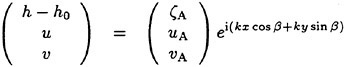
(21)
into the linearized stationary Boussinesq equations:
(22)
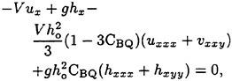
(23)
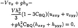
(24)
where ![]() is the wave number and β is the wave propagation angle relative to the ship.
is the wave number and β is the wave propagation angle relative to the ship.
The Taylor expansions of the dispersion relation from the linear wave theory can be given by:
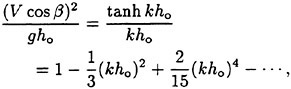
(25)
and of the dispersion relation of the linearized Boussinesq equations by:
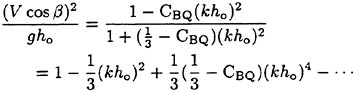
(26)
An approximation of order (kho)4 leads to ![]()
![]() . To demonstrate the influence of CBQ on the dispersion relation, Fig. 2 (a) shows the dispersion relations in graph (a) of the linearized classical (CBQ=0) and modified
. To demonstrate the influence of CBQ on the dispersion relation, Fig. 2 (a) shows the dispersion relations in graph (a) of the linearized classical (CBQ=0) and modified ![]() Boussinesq equations and compares them with that from the linear wave theory for finite depth water. It can be seen that the modified Boussinesq equations are valid for a ratio of wave length to water depth down to a value of 2, practically in the deep-water range. The error relative to the linear wave theory remains within 5%, as shown in graph (b).
Boussinesq equations and compares them with that from the linear wave theory for finite depth water. It can be seen that the modified Boussinesq equations are valid for a ratio of wave length to water depth down to a value of 2, practically in the deep-water range. The error relative to the linear wave theory remains within 5%, as shown in graph (b).

Fig. 2 Comparison of dispersion relations for linear ship waves
Approximation of the Near-Ship Flow
For studying shallow water waves generated by slender ships there exists a well-established method, namely the technique of matched asymptotic expansions, first introduced by Tuck (1966). The basic idea is that the flow field is divided into an outer region (far field) and an inner region (near field) relative to the ship. In each flow region a scale analysis is then performed by selecting suitable scales for all variables, and the resulting simplified forms of the
original governing equations are matched by means of asymptotic multiple-scale expansions in both regions. The asymptotic outer expansion of inner solution for the transverse velocity at ship location can be given by
(27)
disregarding the dynamic effects, see e.g. Mei and Choi (1986), and by
(28)
including the effects of the longitudinal perturbation velocity ![]() as well as of the instantaneous cross-section area S(x, t) which depends on sinkage, trim and local wave elevation
as well as of the instantaneous cross-section area S(x, t) which depends on sinkage, trim and local wave elevation ![]() see e.g. Chen and Sharma (1995).
see e.g. Chen and Sharma (1995).
Using now the Airy pressure to approximate the pressure on the hull surface z=−Τ(x, y):
(29)
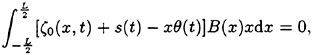
where T(x, y) is the local draft of the ship, the wave resistance can be obtained by a single-integral formulation
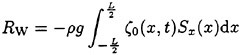
(30)
for still-water wetted surface S(x) and
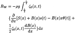
(31)
for instantaneously wetted surface with the local beam B(x).
Due to free heave and pitch, the resulting dynamic vertical force and pitch moment have to vanish. Disregarding inertial effects believed to be small, these equilibrium conditions lead to the following pair of linear algebraic equations:
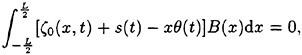
(32)
(33)
for determining the unknown squat, i.e., sinkage s(t) and trim θ(t).
NUMERICAL SOLUTION
Time and Space Discretization
According to the Crank-Nicholson scheme the governing Boussinesq equations are now discretized in time and space. Using the difference operators defined by
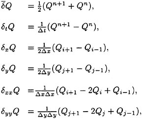
where Q represents any state variables of (h, u, v), the Boussinesq equations turn into a finite-difference formulation as follows:
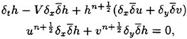
(34)
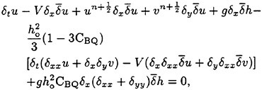
(35)
(36)
The required state values ![]() for the nonlinear terms may be approximated by the state values at the time step n. Based on the Taylor expansion and the linearized Airy equations high-order approximations of these state values can be obtained. Following this treatment the finite difference equations (34–36) in the whole calculation domain form together an algebraic linear equation system. One special feature of this linear equation system is that the associated system matrix is a so-called sparse matrix, i.e., only a small number of its matrix elements are nonzero. To reduce the memory requirement the coordinate storage technique (COO) is applied, i.e., only the nonzero elements and their addresses are stored.
for the nonlinear terms may be approximated by the state values at the time step n. Based on the Taylor expansion and the linearized Airy equations high-order approximations of these state values can be obtained. Following this treatment the finite difference equations (34–36) in the whole calculation domain form together an algebraic linear equation system. One special feature of this linear equation system is that the associated system matrix is a so-called sparse matrix, i.e., only a small number of its matrix elements are nonzero. To reduce the memory requirement the coordinate storage technique (COO) is applied, i.e., only the nonzero elements and their addresses are stored.
Boundary Conditions
In principle there are four kinds of boundaries in the flow problem considered here: (i) the symmetry conditions on the plane y=0; (ii) the no-flux condition v=0 on the channel walls; (iii) the flux condition at the ship location as defined by equations (27–28); and (iv) the no-reflex condition on the open boundary. For the unknown state variables in (i), (ii) and (iii) simple one-sided finite difference schemes from the inner calculation field can be used. For the unknown state variables in (iv) only the outgoing characteristics of the governing equations lead to stable numerical solution. Considering one-dimensional Boussineq equations and disregarding their high-order terms the suitable condition is given by the well-known Sommerfeld condition:
(37)
or
(38)
where σ denotes the outgoing characteristic of the governing equations on the boundary. The associated space difference has to be formed from the inner calculation field. In the present study the eigenvalues of the linearized Airy equations, i.e., Boussinesq equations without high-order terms, are used, i.e., ![]() for the down-stream boundary,
for the down-stream boundary, ![]() for the up-stream boundary,
for the up-stream boundary, ![]() for the open boundary at y=constant>0, and for the
for the open boundary at y=constant>0, and for the ![]() open boundary at y=constant<0, see Jiang (1996).
open boundary at y=constant<0, see Jiang (1996).
Solution Procedure
For given initial conditions (h=ho, u=0, v=0) and numerical towing speed (V* acceleration factor) the resulting linear equation system is iteratively solved by means of a standard Gauß-Seidel method with controllable accuracy. To accelerate the convergence process the overrelaxation method is used. To suppress the numerical oscillations of the solution local and global filtering techniques are implemented in the computer programme.
RESULTS AND DISCUSSION
Model Experiments
The experimental results reported here are from the model experiments conducted in the main towing tank (200 m×9.81 m×1 m) of the Duisburg Shallow Water Towing Tank (VBD). Its water depth can be adjusted to any value from zero to one meter. A Series 60 hull with a block coefficient CB=0.594 and a total weight W=4271 Ν was chosen for the model tests. The model has a length between perpendiculars L=4.689 m, a beam B=0.6252 m, and a draft T=0.25 m. The water depth in the tank was 0.5 m, which leads to a ratio of water depth to ship draft h0/T=2.0, being representative of shallow water dynamics. The wetted hull-surface in quiet water is S=3.77 m2. The towing speeds covered the subcritical, transcritical and supercritical speed range of Fnh from 0.5 to 1.7. The model towed was free to heave and pitch. Due to the non-stationary nature of flow near the transcritical speeds, long time histories of total resistance, sinkage and trim were recorded. The wave profiles on the hull surface were photographically documented. The wave profiles in the tank were obtained by means of wave gauges fixed in the towing tank. All quantities reported here are either at model-scale or non-dimensional.
Trial Computations
A large number of trial computations were performed to find suitable values of time step-size Δt for the given space step-sizes Δx and Δy. In most cases the computation is stable and convergent for the choice of ![]() . For Δx≈Δy used in present study this leads to
. For Δx≈Δy used in present study this leads to ![]() . After test runs in the speed range Fnh from 0.5 to 1.8 a time step size
. After test runs in the speed range Fnh from 0.5 to 1.8 a time step size ![]() was used in the computations reported here. Δx takes the value of
was used in the computations reported here. Δx takes the value of ![]() and
and ![]() . The length of the calculation domain is 10 times the ship length, namely,
. The length of the calculation domain is 10 times the ship length, namely, ![]() ahead of the ship and
ahead of the ship and ![]() behind the ship. For 2000 time steps it runs ca. 3 CPU hours for one speed in a HP Workstation.
behind the ship. For 2000 time steps it runs ca. 3 CPU hours for one speed in a HP Workstation.
Wave Resistance and Wave Patterns
The calculated specific wave resistance of the Series 60 hull in the configuration identical to the model tests is shown in Fig. 3, as a function of the depth Froude number. The wave resistance curve is characterized by a slow increase in the subcritical range, then by a strong rise accompanied by oscillations of steeply increasing amplitude (shown by error bars) at the transcritical speed range, and finally by a slow drop in the supercritical range. Representative wave patterns in these three speed ranges are visualized as density plots in Fig. 4. At subcritical speeds, here for Fnh=0.8 in graph (a), the steady wave system is close to a Havelock wave pattern. At
transcrical speeds, here for Fnh=1.0 in graph (b), the wave system is characterized by an unsteady wave pattern with solitons propagating ahead of the ship and responsible for the oscillations of the ship as well as of the resistance. At supercritical speed, here for Fnh=1.5 in graph (c), the wave system is again steady but comprises only divergent waves within the angle of ± arcsin ![]() corresponding to the Mach angle at hypersonic flow in gas dynamics.
corresponding to the Mach angle at hypersonic flow in gas dynamics.
Comparison of the Integral Quantities
Fig. 5 compares the calculated (○) versus measured (+) mean values of specific total resistance (a), sinkage (b), and trim (c). The calculated total resistance is the sum of the calculated wave resistance and the estimated viscous resistance being equal to the frictional resistance according to the ITTC 1957 correlation line multiplied by a form factor 1+k=1.175, which is derived from resistance measurements at low speeds using the standard Hughes-Prohaska technique. The general observation is that a good agreement between calculations and model measurements was achieved in the whole speed range for all quantities compared. Looking more closely, one can observe: (i) The agreement of the resistance (a) near bifurcation points, i.e., the transition from steady solution to unsteady one at Fnh≈0.9 or vice-versa at Fnh≈1.2 is not so good as elsewhere. Time histories of measurements showed that the asymptotic state can not be achieved within the limited tank length near these points. Numerical simulations showed that the calculations depended on the time step-size. To get more accurate explanations further experimental as well as numerical effort is required, (ii) The agreement for sinkage in the supercritical range is not so good as well. It also needs further examination.
Comparison of the Wave Records in the Tank
To validate the calculated wave patterns four wave gauges were fixed in the tank at y=0.5, 1.0, 2.45, and 4.41 m, respectively. The recorded time histories of the wave elevation are then transformed to the relative coordinate system moving with the ship. Due to the unsteady nature of the wave pattern in the transcritical speed range the longitudinal wave cuts are not equivalent to the time histories at the wave gauges. Therefore, the wave elevation at the corresponding wave gauges is restored as a function of xWG=xWG(nMΔt)−(n−nM)ΔtV, where nΜΔt is the starting time for measurements. Unfortunately, due to the different acceleration in model test and numerical calculation nMΔt cannot be used in the numerical towing tank. In the present study the prominent event of the first soliton peak passing the wave gauges is used to reconstruct the suitable time-space transformation. Fig. 6 compares the calculated wave records with those measured at the critical speed Fnh=1.0. The main observations are: (i) The agreement is remarkable not only near the ship (responsible for the good agreement of the integral quantities) but also ahead of the ship as well as in the wake upto ![]() ship length, validating the computer program developed in the present study, (ii) The small phase shift could be caused by different accelerations in model tests and calculations, (iii) The relatively large difference beyond two ship lengths behind the ship may be due to viscous effects or a hydraulic jump in the tank not simulated in the computation.
ship length, validating the computer program developed in the present study, (ii) The small phase shift could be caused by different accelerations in model tests and calculations, (iii) The relatively large difference beyond two ship lengths behind the ship may be due to viscous effects or a hydraulic jump in the tank not simulated in the computation.
To show the effect of the different representations of the near-ship flow, Fig. 7 compares the wave records calculated by using the classical slender-body theory in equation (27) (solid lines) and by using the modified slender-body theory in equation (28) (dashed lines). No noticeable influence on the solitary waves and on the wake waves far behind the ship can be observed. The difference alongside the ship can also be neglected. Fig. 8 demonstrates the effect of coefficient CBQ on the wave pattern. As expected, in comparison to the classical Boussinesq equations of CBQ=0 (solid line) the modified Boussinesq equations of ![]() allow small wave lengths in the wake. But it has no influence on the long solitary waves. Based on the comparisons in Fig. 7 and 8 the numerical results reported in Fig. 3, 4, 5 and 6 were all calculated in the computer module using the classical Boussinesq equations in the far field and the classical slender-body theory in the near field.
allow small wave lengths in the wake. But it has no influence on the long solitary waves. Based on the comparisons in Fig. 7 and 8 the numerical results reported in Fig. 3, 4, 5 and 6 were all calculated in the computer module using the classical Boussinesq equations in the far field and the classical slender-body theory in the near field.
CONCLUSIONS
An implicit difference method based on the Crank-Nicholson scheme was implemented to approximate the shallow-water wave equations of Boussinesq type. To simulate the wave generation by a slender ship in a shallow-water channel the technique of matched asymptotic expansions was applied. Calculations showed that the modifications of the Boussinesq equations by improving the dispersion relation and of the slender-body theory by means of taking account of the high-order dynamic effects have no significant influences on the numerical results reported here. Satisfactory agreement between calculations and model experiments was achieved not only for the integral quantities, such
as wave resistance, sinkage and trim, but also for field quantities, such as wave profiles in the tank.
ACKNOWLEDGMENTS
The author is grateful to Dipl.-Ing. H.Nguyen Duc, cand. arch. nav. R.Henn, and Dipl.-Ing. N.Stuntz of the Institute of Ship Technology at the Mercator University Duisburg for their assistance in computer programming and in conducting the model experiments, respectively. He is also grateful to Professor Dr.-Ing. Sharma for his continuous support.
REFERENCES
Chen, X.-N. and Sharma, S.D., “A Slender Ship Moving at a Near-critical Speed in a Shallow Channel,” Journal of Fluid Mechanics, 1995, Vol. 291, pp. 263–285.
Choi, H.S. and Mei, C.C., “Wave Resistance and Squat of a Slender Ship Moving Near the Critical Speed in Restricted Water,” Proceedings of the 5th International Conference on Numerical Ship Hydrodynamics, 1989, pp. 439–454.
Dingemans, M.W., “Water Wave Propagation over Uneven Bottoms,” Advanced Series on Ocean Engineering, Vol. 13, World Scientific Publishing Co. Pte. Ltd, 1997.
Graff, W., Kracht, A. and Weinblum, G., “Some Extensions of D.W.Taylor’s Standard Series”, Transactions of Society of Naval Architects and Marine Engineers, Vol. 72, 1964, pp. 374–401.
Helm, K., “Effects of Channel Depth and Width on Ship Resistance (in German),” Hydrodynamische Probleme des Schiffsantriebs, Part 2, ed. G.Kempf, Verlag Oldenburg, Munich and Berlin, 1940, pp. 144–171.
Jiang, T., “Simulation of Shallow Water Waves Generated by Ships Using Boussinesq Equations Solved by a Flux-Difference-Splitting Method,” Proceedings of the 11th Int. Workshop on Water Waves and Floating Bodies, Hamburg, 1996.
Jiang, T., Sharma, S.D., and Chen, X.-N. 1995, “On the Wavemaking, Resistance and Squat of a Catamaran Moving at High Speed in a Shallow Water Channel,” Proceedings of the 3rd International Conference on Fast Sea Transportation FAST’95, Lübeck, Travemünde, 1995, pp. 1313–1325.
Mei, C.C., “The Applied Dynamics of Ocean Surface Waves,” Advanced Series on Ocean Engineering, Vol. 1, World Scientific Publishing Co. Pte. Ltd, 1989.
Mei, C.C. and Choi, H.S., “Forces on a Slender Ship Advancing near Critical Speed in a Wide Canal,” Journal of Fluid Mechanics, Vol. 179, 1987, pp. 59–76.
Madsen, O.S. and Mei, C.C., “The Transformation of a Solitary Wave over an Uneven Bottom,”, Journal of Fluid Mechanics, Vol. 39, 1969, pp. 781–791.
Madsen, P.A., Murray, R., and Sørensen, O.R., “A New Form of the Boussinesq Equations with Improved Linear Dispersion Characteristics, Part 1,” Coastal Engineering, Vol. 15, 1991, pp. 371–388.
Nwogu, O., “Alternative Form of Boussinesq Equations for Nearshore Wave Propagation,”, Journal of Waterway, Port, Coastal Engineering, Vol. 119, No. 6, 1993, pp. 618–638.
Pedersen, G., “Three-Dimensional Wave Patterns Generated by Moving Disturbances at Transcritical Speeds,”, Journal of Fluid Mechanics, Vol. 196, 1988, pp. 39–63.
Schröter, A., “Nichtlineare Zeitdiskrete See-gangssimulation im Flachen und Tieferen Wasser (in German),” Institut für Strömumngsmechanik and Elektronisches Rechnen im Bauwesen der Universität Hannover, Report No. 42, 1995.
Tuck, E.O., “Shallow Water Flows Past Slender Bodies,” Journal of Fluid Mechanics, Vol. 26, 1966, pp. 81–95.
Thews, J.G. and Landweber, L. 1935, “The Influence of Shallow Water on the Resistance of a Cruiser Model,” US Experimental Model Basin, Navy Yard, Washington, DC, Report No. 408.
Wehausen, J.V. and Laitone, E.V., “Surface Waves,” Handbuch der Physik, Springer, Vol. 9, 1960.
Witting, J.M., “A Unified Model for the Evolution of Nonlinear Water Waves,” Journal of Computational Physics, Vol. 56, 1984, pp. 203–236.
Wu, D.-M., and Wu, T.Y., “Three-Dimensional Nonlinear Long Waves Due to Moving Surface Pressure,” Proceedings of the 14th Symposium on the Naval Hydrodynamics, Ann Arbor, 1982, pp. 103–129.
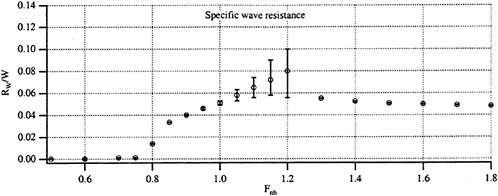
Fig. 3 Calculated wave resistance of a Series 60 hull moving along the centerline of a shallow-water channel at water-depth ![]() and channel-width
and channel-width ![]()
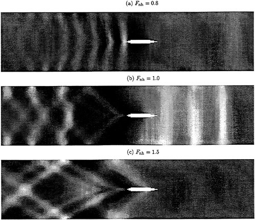
Fig. 4 Calculated wave patterns of a Series 60 hull at subcritical (a), critical (b), and supercritical (c) speeds in a shallow-water channel at water-depth ![]() and channel-width
and channel-width ![]() visualized as density plots
visualized as density plots
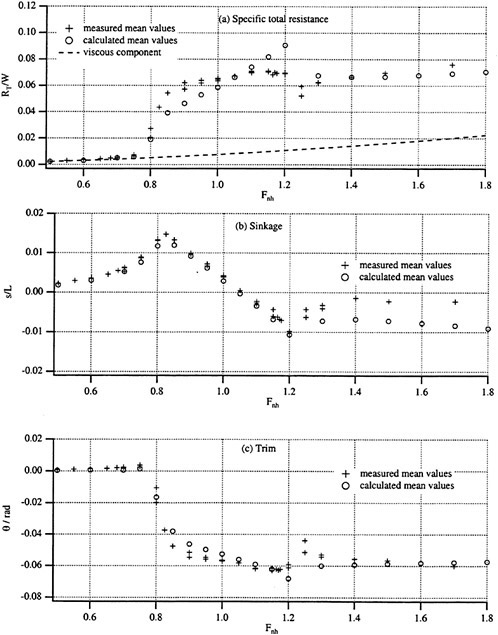
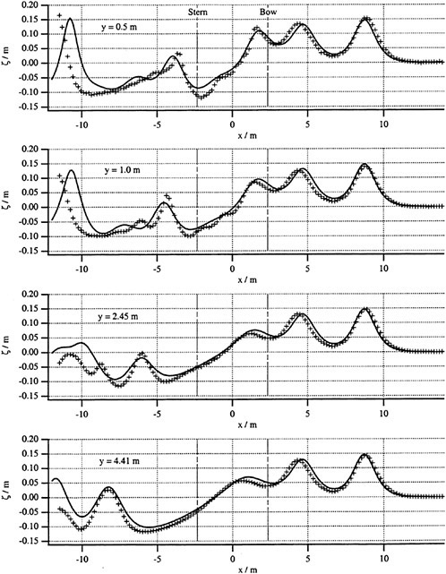
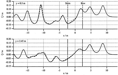
Fig. 7 Comparison of wave profiles calculated by using classical (solid line) and modified (dashed line) slender-body theory in the near field at the critical speed
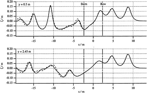
Fig. 8 Comparison of wave profiles calculated by using classical (solid line) and modified (dashed line) Boussinesq equations at the critical speed
Case Studies of Hurricane and Winter Storms Using a New Coastal Wave Model
R.Lin (Naval Surface Warfare Center, Carderock, USA),
W.Perrie (Bedford Institute of Oceanography, Canada)
Abstract
The most critical factor for Naval operations in the nearshore domain is the correct estimation of environmental factors such as winds, waves, currents and storm surge events. Moreover, ship motions are strongly impacted by the inhomogeneity of the sea surface. In finite depth water or shallow water, the mechanisms that influence the sea surface, including its homogeneity or inhomogeneity, become more complex than the associated deep water mechanisms. In the former case, water depth becomes important, and is not only functionally related to spatial gradients, per se, but water depth is also functionally related to temporal changes, which are dictated by appropriate formulations for the nonlinear source function and wave breaking dissipation. These “appropriate” formulations are not presently incorporated in wave modeling technologies. In addition, the influence of surface driven currents, which is very important for many littoral warfare applications, will effectively refract directional wave spectra, promote local breaking, alter the momentum transfers both in the air-sea boundary and also internally within the spectral frequencies. Thus, to accurately estimate the appropriate wave characteristics, needed for naval operations, the spectral wave model must include all physical mechanisms in temporal and spatial scales necessary to accurately resolve these effects [1,2,3,4]. Our new coastal wave model achieves this objective by incorporating all the recent advances:
-
We apply the action conservation equation instead of an energy transfer equation. Moreover, the model simulates the divergence which causes physical dispersion and easily incorporates wave-current interactions [1,2,3,4].
-
To solve the action conservation equation, we developed a semi-implicit scheme with a directional filter which not only overcomes the Gibbs instability, but runs twice as fast as previously published wave models [1,3].
-
We incorporated the Phillips’ resonant wind-wave generation mechanism, resulting in more realistic representation of growing wind-seas at off-wind angles.
-
We use a more well posed formulation for the nonlinear wave-wave interaction source function that:
-
whereas Phillips’ mechanism [5] breaks down over shallow water, and wave models often continue to use this mechanism, we found a new mechanism—the wide band instability—which we implement in our model [6,7];
-
whereas WAM and other wave models parameterize the nonlinear source function Snl, we explicitly calculate Snl by extending [8,9]’s Hamiltonian formulation to shallow water, which gives a simple formulation and allows an efficient accurate quasi-one dimensional representation of Snl [10].
-
whereas WAM and other wave models consider only 4-wave interactions, we also consider higher-order 5-wave interactions for large amplitude three-dimensional waves [11].
-
In this study, we apply our new coastal wave model to finite depth water to simulate the spectral wave transformations occurring during well documented hurricane and winter storm events occurring during the DUCK90 field experiment. Our wave model is also coupled to a coastal current model [12]. The input functions for the coupled wave-current model are wind and bottom distributions. The outputs are current distributions and energy spectra distributions (wave height and propagating directional distributions). For the storms considered here, we show that the model is not only highly accurate, but also very efficient. This model can provide real-time forecasts.
1 INTRODUCTION
In shallow water depths, the wavelengths of the wind—generated waves cannot become extremely long because 4-wave interactions involve the four approximately equivalent waves (Phillips mechanics) which decrease with water depth [6,13]. However, if long waves were generated in deep ocean and subsequently propagate to shallow water, one may be able to observe them in shallow water, although bottom dissipation and wave—breaking will normally quickly eliminate them. Moreover, the presence of short waves in shallow water and their interactions with the long waves, may allow the long waves to extract energy from the short waves and therefore maintain themselves for some period of time and even longer wavelengths may result [6,10]. Furthermore, another cause of long waves in shallow water is through wave-current interactions. In strong current conditions, frequency shifts due to wave-current interactions [2,4], may result in lengthening of wavelengths, beyond what one expects to observe in shallow water.
Observed wave data can indeed show that, during hurricanes, winter storms, very long waves can be found in very shallow water, provided the shallow water is connected with deep water and swell propagates from the open ocean to the shallow water continuously, with the wind is blowing onshore, from the open ocean to the land. An example is the hurricane storm occurring during 10–12 October 1990 off North Carolina. Measured spectra were recorded in 13 m depth water, 2 km offshore from Duck, North Carolina at 20:25 PM on 12 October 1990. The peak frequency is about 0.076 Hz, which corresponds to a wavelength of about 150 m, with a waveheight of 2.40 m, as shown in Fig. 1 and reported in [14]. This wavelength can strongly resonate with naval ships.
To predict surface waves accurately in shallow water, especially during winter storms or hurricanes is a very great challenge because in shallow water, the mechanics are entirely different to those of deep water. Although 4-wave interactions (2-dimensional wave-wave interactions) dominate in deep ocean, they decrease with water depth [6,13]. In shallow water, wave-current interactions [2], the 5-wave interactions (3-dimensional wave-wave interactions) of [6,11], and long wave—short wave interactions of [6,10] become more important. The present state-of-the-art model WAM, as described by [15], is based on deep water theory, as is a variation of the WAM model, the WAVE-WATCH model of [16]. The latter has additional problems due to its unconditional numerical instabilities, as noted by [1,2,3,4].
Recently, [17] developed a shallow water wave model, which is based on 3-wave interactions, the so—called ‘quasi-resonant interactions’. They claim that 3-wave interactions dominate in shallow water. However, they assume the shallow water dispersion relation,
(1)
where ω is frequency, ![]() is wave number, k is absolute value of
is wave number, k is absolute value of ![]() and d is water depth. The resonant condition for 3-wave interactions is:
and d is water depth. The resonant condition for 3-wave interactions is:
(2)
From simple mathematics, these quasi-resonant conditions request that the 3-wave interactions are parallel. However, parallel wave-wave interactions are identically zero because the coefficients of interactions exactly cancel [18]. Thus the model of [17] is based on nonexistent theory.
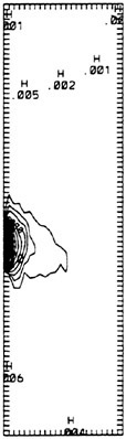
Fig. 1. Energy spectrum observed at 20:25 PM on 12 October 1990 during the DUCK90 Experiment [14]. The vertical coordinate is the wave propagation angle, which varies from 2.7273° to 358.6363°. The horizontal coordinate is frequency, varying from 0.0659 Hz to 0.2344 Hz. The offshore direction is at 0°, which is about 70° relative to true north.
By comparison our new model is based on
-
not only the four roughly equivalent waves involved in 4-wave interactions (Phillips’s mechanics), but also long wave and short wave [6,7], and three-dimensional 5-wave interactions [11,19].
Our new model also considers the interaction of wind input Sin and wave breaking Sds with the nonlinear source function Snl [20]. Therefore, our new wave model is suitable for both deep ocean and coastal regions.
2 The New Coastal Wave Model
(A) The Basic Equation (Action Conservation Equation):
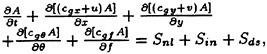
(3)
where A is action density spectrum; t is time, x, y are the horizontal coordinates, θ is the propagation angle; f is the frequency; Snl is the nonlinear source function; Sin is the wind input function; Sds is the wave dissipation function; cgx+u, cgy+v, cθ, cf are the propagation velocities of action density spectrum components in x, y, θ and f space, respectively.
(B) Nonlinear Kinematics:
As [2,4] described, the nonlinear kinematics is very important in shallow water, especially when there is current. For nonlinear kinematics, the dispersion relation is [21]; [2]:
(4)
and the space velocities are:
(5)
(6)
(7)
(8)
where ![]() .
.
(C) Nonlinear source function (Snl):
To calculate the Snl, we use an explicit computation of the integral, the so—call RIA formulation [22], which is based on the Hamiltonian variational principle. Because the resonant solution is highly nonlinearly distributed, we are able to reduce the original six-dimensional integration to a quasi-line integration. The latter is 1000 times faster than the ‘EΧΑCΤ-NL’ formulation of [23], and 100 times faster than [24,25], but still 20 times slower than DIA [26,27], as implemented in WAM. However, unlike DIA, the RIA obtains a highly accurate solution, with an error of less than 5%. The nonlinear action transfer rate by RIA, as given in [22], is the following:
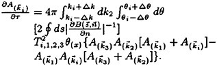
(9)
where coefficient Ti,1,2,3 is defined in [6].
The DIA formulation is valid only for deep water, and even there it ignores much of the complexity of nonlinear wave—wave interactions. Alternately, the RIA formulation for Snl is suitable for both shallow and deep water. Moreover, when the water becomes shallow, 4-wave interactions due to roughly equivalent gravity waves become less dominant, whereas 4-wave interactions involving 3 gravity waves and one one long wave become dominate. The long waves can be swell, bottom topography waves, or edge waves [6,13]. When waves are very steep, the higher-order three-dimensional waves may dominate [28,29,30,11], such as 5-waves. Finally, when the 4-wave interactions become coupled with 5-wave interactions and when the waves are very steep and the angular propagation spread is very narrow, the three-dimensional wave-wave interactions may dominate even in deep water [31,19]. In conclusion, shallow water Snl is far more complicated than deep water Snl. Therefore a parameterization method, such as DIA, cannot possibly simulate Snl. An explicit detailed integration is necessary to calculate Snl.
(D) Wind Input and Wave Breaking (Sin+Sds):
Typical formulations for wind input Sin and wave breaking dissipation Sds assume a form such as E(f)fm where m is about 2. By contrast, our model allows m to vary with spectral maturity, where m is associated with direct and inverse cascades in the spectrum, following [9]. Direct cas-
cades consist of energy fluxes from low to high frequencies, whereas inverse cascades consist of energy fluxes from high frequencies to low frequencies [20].
3 The Model Results and Observed Data
In this section, we simulate a hurricane storm and a typical winter storm, as observed during DUCK90 Experiment [14]. The wind data was measured at the end of the pier at the Duck experimental site. All wave spectra were measured by bottom pressure transducers, as described by [14], at the Duck site, 2 km offshore, in 13 m depth. The experimental site is shown in Fig. 2 from [14]. True North is 70° from offshore, which is taken as 0° in the wave spectra coordinates.
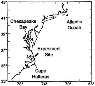
Fig. 2 Experiment site from [14]
(A) Hurricane Case:
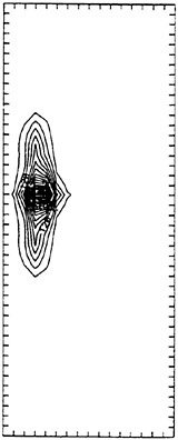
Time series for the wind speeds and directions are shown in [14]. For the period beginning 36 hours before the spectrum of Fig. 1, local winds are light, first 10 m/s to the southeast (SE), then 5 m/s to the northeast (NE) and finally 6 m/s to east-southeast (ESE). Except for very short time-periods during this interval, when low 5 m/s winds blow from land to ocean, most winds are onshore, from open ocean to the land. Effectively, this storm qualifies as a hurricane case because wave generation occurs in the deep waters of the open ocean, and the waves of Fig. 1 represents only small old swell remnant spectrum, slowly decaying as it propagates through the shallow water of Duck, North Carolina, far from the position of its original generation. The observed wave spectrum at 20:25 on 12 October 1990 is shown in Fig. 1. The swell waves have propagated from the deep water to shallow water, each interacting with three local short wind waves. A simulation of this case, using our new coastal wave model, is shown in Fig. 3. The peak frequency of the initial spectrum is 0.2 Hz at deep water is showed in Fig. 3a. After 36 hours, using the wind time series reported by [14], we obtained the final spectrum, which is showed in Fig. 3b. Its peak frequency of the spectrum has decreased to about 0.075 Hz and the wave height is 2.65 m. Therefore, our model results agree well with the observation data in Fig. 1, in peak frequency and wave height.
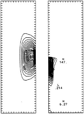
Fig. 3. Results from our new coastal wave model, assuming the frequency and angle domains as in Fig. 1: peak frequency evolves from an assumed initial value of 0.2 Hz in Fig. 3a at 08:25 on 11 October 1990 to a final value of 0.076 Hz at 20:25 on 12 October 1990, in Fig. 3b.
However, Fig. 1 is the only observed data for this hurricane event available to us. A detailed modeling of this storm must involve high-quality gridded wind fields for the northwest Atlantic, time-series of observed wave spectra for the entire storm, from sites in shallow water as well as deep water, and implementation of the wave model for a reasonably fine-mesh grid (20 km or better, for a mesoscale event such as this hurricane) for the northwest Atlantic. As our simulation has not
had this detail, it is impossible to differentiate between the two opposite theories: [6,14] if we only simulated this hurricane case. We expect that both may obtain results somewhat comparable to measured data in Fig. 1. Implicit in the simulation based on [6] is the claim that the long waves are due to the 3-wave interacting with swell. By contrast, [14] implicitly claim that this is an extremely shallow water effect, and that the 3-wave interactions generate the long waves.
However, we must note that the waves of this so-called hurricane are much too low to be associated with real hurricane conditions. For example, Hurricane Luis propagated across the Grand Banks of Newfoundland in September 1995, with maximum wave heights in excess of 30.0 m and maximum winds in the 25–30 m/s range. Therefore, the so-called hurricane case of this study is really only the small old swell remnant spectra from a distant hurricane storm in deep ocean, as noted above. This is not local shallow water wind generated waves.
(B) Winter Storm:
The winter storm case occurred during the DUCK90 experiment (specifically 09:04 25 to 00:04 26 October 1990) in the same location as the hurricane event described above. As presented in [14], local winds were strong, as measured from the Duck pier. They were initially 15 m/s to the NNE, then 20 m/s to the NNW, from the land to ocean. For such high wind storm events, persisting for a long time, the waves should feel the bottom and thus should be considered shallow water waves. Our model allows an automatic consideration of possible shallow water effects in this storm. Observed wave spectra are presented in Figs. 4a–d.
The peak frequency of the spectrum in Fig. 4b is a lot higher than that of in Fig. 4a. Furthermore, the propagation direction of Fig. 4a is different from that of Fig. 4b. Obviously the spectrum in Fig. 4a consists of very weak old swell, whereas the spectrum in Fig. 4b is newly generated wind-waves. Moreover, the peak frequency of the spectrum in Fig. 4c is lower than that of Fig. 4b, but the wave height in Fig. 4c is greater than that of Fig. 4b. This is repeated in Fig. 4d, which reports lower peak frequency and higher wave height than the spectrum of Fig. 4c. As the dominant wave propagation direction in Figs. 4b–d corresponds approximately to the wind direction, the wave spectra is wind-generated and wind-driven in these figures.
According to [6], 4-wave interactions decrease with decreasing water depth. Therefore, the wavelength of these shallow water waves, in case 2, should be shorter than that of the hurricane case, in case 1. This is consistent with the observed data, as reported here and in the previous section. We note that this contradicts alternate theories, suggesting the opposite, that 4-wave interactions increase as water depth decreases.
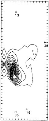
Fig. 4a Observed spectrum at 01:34 on 25 October 1990. Peak frequency is 0.12 Hz, and wave height is 0.70 m.
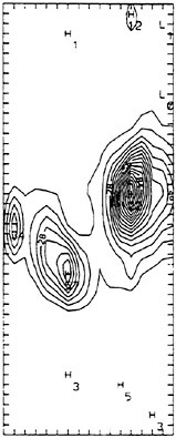
Fig. 4b Observed spectrum at 09:04 on 25 October 1990. Peak frequency is 0.23 Hz and wave height is 1.06 m.
In the following discussion, we compare the model results with the observed data quantitatively and qualitatively. The results of our new coastal wave model are shown in Fig. 5, starting with the spectra of Fig. 4b as our initial spectrum. We achieve good agreement between model results in Figs. 5a–b and the corresponding observed data in Figs. 4c–d, in terms of peak frequencies and wave heights.
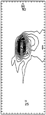
Fig. 4c Observed spectrum at 16:34 on 25 October 1990. Peak frequency is 0.16 Hz and wave height is 2.12 m.
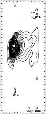
Fig. 4d Observed spectrum at 00:04 on 26 October 1990. Peak frequency is 0.12 Hz and wave height is 3.83 m.
As noted above, very long waves present in Fig. 1 from the hurricane storm are not generated locally in the shallow water of the duck site. These swell waves propagate from deep water in the open ocean, far from Duck, where they are generated during the active hurricane growth and evolution stages. In shallow waters near Duck, these swell spectra interact with local wind—generated waves, which may provide them with energy from wind waves, and slight down—shifting in frequency.
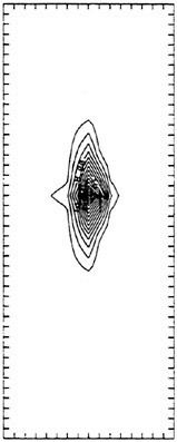
Fig. 5a Wave model spectrum, corresponding with Fig. 4(c), with peak frequency is 0.16 Hz and the wave height, 2.27 m.
Unlike the hurricane storm of case 1, the winter storm of case 2 is basically wind—generated waves. The wind speed of case 2 is more than twice as large as that of case 1. In case 2, the wind is offshore, from the land to open ocean, but the wind is strong and continuous, which should be reflect a shallow water effect. The peak frequency in case 2 is much higher than that of case 1. In any case, the alternate theory, which suggests that 4-wave interactions increase rapidly with decreasing water depth, cannot tune to both cases.
4 Conclusions
Our new coastal wave model was shown to agree well with the observed data for both the hurricane storm and the winter storm cases of this study, with respect to peak frequency and wave height.
Long waves were observed in very shallow water with very light local winds, blowing from the open ocean to the land, in the hurricane storm of case 1. The generation of these long waves occurs in deep water. These swell waves are generated in the open ocean and then propagate into shallow water, where they interact with the locally generated wind—waves. Much shorter waves were observed at the same location in case 2, with strong offshore winds from the land to the open ocean. These short waves were generated locally and reflect shallow water effects.
Comparing these two cases, it is easy to see that 4-wave interactions (4 roughly equivalent waves) decrease with water depth [6,13]. In addition, the interactions of three gravity waves and one long wave dominate when the water is shallow and the slope of the long wave is steep. It is important to note that our conclusion is in contrast to previous studies, which claim that 4-wave interactions increase with decreasing water depth, e.g., [14].
Acknowledgements. This research is funded by Base Enhancement Wave Prediction Program of the Office of Naval Research. The wave modeling program at BIO is funded by the Federal Panel on Energy Research and Development (Canada) under Project 534201. We thank Dr. Herbers for making the observed data from Duck90 available to us.
References
[1] Lin, R.Q. and N.E.Huang, 1996a: A New Coast Wave Model: Part I: Numerical Method. J. of Phys. Oceanogr. Vol. 26, 833–847.
[2] Lin and N.Huang, 1996b: The Goddard Coastal Wave Model. Part II. Kinematics. J. of Physical Oceanography, Vol. 26, No. 6, 848–862.
[3] Lin, R.Q., 1998a: Reply Comments on Part I by Tolman et al. J. of Phys. Oceanogr. In press.
[4] Lin, R.Q., 1998b: Reply Comments on Part II by Tolman et al. J. of Phys. Oceanogr. In press.
[5] Phillips, O.M., 1960: On the dynamics of unsteady gravity waves of finite amplitude. J. Fluid Mech., 9, 193–217.
[6] Lin, R.Q. and W.Perrie, 1997a: A New Coastal Wave Model, Part III. Nonlinear Wave-wave Interactions. J. of Physical Oceanography, Vol. 27, No. 9, 1813–1826.
[7] Lin, R.Q. and W.Perrie, 1997c: On the Mathematics and Approximation of the Nonlinear Wave-wave interactions. In Vol. 17, Advances in Fluid Mechanics, Ed. W.Perrie. Computational Fluid Mechanics, Southampton. 27 pp.
[8] Zakharov, V.E., 1968: Stability of periodic waves and finite amplitude on the surface of deep fluid. Zhurnal Prikladnoi Mekhaniki Tekhnicheskoi Fiziki, 3, No. 2, 80–94.
[9] Zakharov, V.E., 1991: Inverse and direct cascade in wind-driven surface wave turbulent and wave-breaking. In Breaking Waves IUTAM Symposium, M.L.Banner and R.H.J.Grimshaw (Editors), Sydney, Australia. 69–91.
[10] Lin, R.Q. and W.Perrie, 1998b: A New Coastal Wave Model. Edge Wave. Submitted to Phys. Fluid
[11] Lin, R.Q. and Perrie, 1997b: A New Coastal Wave Model. Part V. Five-Wave Interactions. J. of Physical Oceanography, Vol. 27, No. 10, 2169–2186.
[12] Huang, R.X. and R.Q.Lin, 1997: A free surface ocean circulation model with fresh water. Documentation.
[13] Zakharov, V.E., 1998: Weak nonlinear Waves on the Surface of an Ideal Finite Depth Fluid. Amer. Math. Soc. Transl. Vol 182, 167–197.
[14] Herbers, T.H.C. and R.T.Guza, 1994: Nonlinear wave interactions and high-frequency seafloor pressure, J. of Geophy. Res. Vol. 99, 10035–10048.
[15] Günther, H., Hasselman, S., P.A.E.M.Janssen, 1993: The WAM model cycle4. DKRZ WAM Model Documentation.
[16] Tolman, H.L., 1992: Effects of Numerics on the physics in a third-generation wind-wave model. J. Physical Oceanography, Vol. 22, 1095–1111.
[17] Herbers, T.H.C., S.Elgar, and T.Guza, 1993: Infragravity-Frequency (0.005–0.05 Hz) Motions on the Shelf. Part I. forced Waves. J. of Physical Oceanography, Vol. 24, 919–927.
[18] Zakharov, V.E. and E.Shulman, 1980: Degenerative Dispersion law, motion invariants and kinetic equation, Physica D, 192–202.
[19] Lin, R.Q. and M.Y.Su, 1998: Three-dimensional Wave-wave Interactions in Deep Water. Submitted to J. Fluid Mech.
[20] Perrie, W. and R.Q.Lin, 1998: On Parameterizations Wind and Wave-Breaking Dissipation. Submitted to J. of Physical Oceanography.
[21] Whitham, G.B., 1974: Linear and nonlinear Waves, John Wiley & Sons, New York, 628 pp.
[22] Lin, R.Q. and W.Perrie, 1998a: A New Coastal Wave Model. Part IV. Nonlinear Source Function. Submitted to J. of Geophys. Res.
[23] Hasselman, S. and K.Hasselman, 1981: A symmetrical method of computing the nonlinear transfer in a gravity—wave spectrum. Hamb. Geophys. Einzelschriften Reihe A: Wiss. Abhand., 52, 138 pp.
[24] Tracy, B.A. and D.T.Resio, 1982: Theory and calculation of the nonlinear energy transfer between sea waves in deep water. WIS REP. 11, US Army Engineering Waterways Experiment Station, Vicksburg, MS. 50 pp.
[25] Resio, D. and W.Perrie, 1991: A numerical study of nonlinear energy fluxes due to wave-wave interactions. Part I. Methodology and basic results. J. Fluid Mech., 223, 603–629.
[26] Hasselman, S., K.Hasselman, J.H.Allender, T.P.Barmett, 1985: Computations and parameterizations of nonlinear energy transfer in gravity-wave spectrum. Part II: Parameterizations of the nonlinear energy transfer for application in wave models. J. of Physical Oceanography, 15, 1378–1391.
[27] Hasselman, S. and K.Hasselman, 1985: Computation and parameterizations of the nonlinear energy transfer in a gravity-wave spectrum. Part I: A new method for efficient computations of the exact nonlinear transfer integral. J. Physical Oceanography, 15, 1369–1377.
[28] McLean, J.W., 1982: Instabilities of finite-amplitude gravity waves on water of finite depth. J. Fluid mech., Vol. 114, 331–341.
[29] Su, M.Y., 1982a: Three dimensional deep-water waves part I, Experimental measurement of skew and symmetric wave patterns, J. Fluid Mech., Vol. 124, 73–108.
[30] Su, M.Y., 1982b: Evolution of groups of gravity waves with moderate to high steepness, Phys. Fluids, Vol. 25, 2167–2174.
[31] Su, M.Y. and W.Green, 1984: Coupling two-and three-dimensional instabilities of surface gravity waves. Phys. Fluids, Vol. 27, 2595–2597.
DISCUSSION
M.Ohkusu
Kyushu University, Japan
We are interested in predicting waves caused by storms in a specified bay. Is your new model able to account for refraction and reflection of waves to predict the storm waves in a bay whose shape and bottom topography are specified?
AUTHORS’ REPLY
Our new model includes refraction and reflection. These two effects are calculated through:
-
Action fluxes, which include wave-current interactions, through the action conservation equation (Lin and Huang, 1996, Lin, 1998). These action fluxes depend on the bottom topography, and spectrum.
-
Nonlinear wave-wave interactions, as presented in Lin and Perrie (1997). The refraction and reflection of waves therefore also depend on the shape of the waves, the frequency domain, wave amplitude, and bottom topography, because these are important factors in estimating nonlinear wave-wave interactions.
-
Coastal boundaries, which define the character of the boundaries. For example, if the boundary is smooth, then refraction is strong. If the boundary is rough, then the waves will be absorbed by the boundary. Reflection also depends on the angle of incidence: whether the boundary is straight, or tilted.
References
[1] Lin, R.-Q. and N.Huang, 1996: The Goddard Coastal Wave Model. Part II. Kinematics. J. of Physical Oceanography, Vol. 26, No. 6, 848–862.
[2] Lin, R.-Q., 1998: Reply Comments on Part II by Tolman et al., J. of Phys. Oceanogr., Vol. 28, No. 6, 1309–1318.
[3] Lin, R.-Q. and W.Perrie, 1997: A New Coastal Wave Model, Part III. Nonlinear Wave-wave Interactions. J. of Physical Oceanogr., Vol. 27, No. 9, 1813–1826.


