
Advancements of the Large-Eddy Simulation for Turbulent Flow Over Complex Bluff Bodies
S.Jordan (Naval Undersea Warfare Center, USA)
ABSTRACT
The present investigation discusses the resolution of the turbulent vortical motion behind two bluff bodies. The LES results of the cylinder wake at Reynolds number of 5,600 showed good comparisons to the published experimental data in terms of the global and local wake characteristics such as the drag and base pressure coefficients, shedding frequencies, near wake structure, and the Reynolds stresses. Qualitatively, the time-averaged Reynolds stresses of the formation region revealed similar symmetric characteristics over the range 525 ≤Re≤140,000. The NACA 0018 hydrofoil simulation was performed at a Reynolds number of 35,000 and a zero angle-of-attack. Although the instantaneous flow is massively separated over most of the trailing edge (by evidence of the formed large-scale vortical structures), it does not transition to turbulence until near the tip.
1. INTRODUCTION
Most fluid dynamic problems in the Navy involve very complex behaviors that cannot be accurately simulated using simple computational methods. Generally, the geometric topologies are quite arbitrary and require special consideration when attempting to predict the associated flow. The flow itself is commonly unsteady, incompressible and very turbulent. An excellent example of these characteristics is the turbulent wake behind a complex bluff body. Comprehensive studies of the vortical formations and the subsequent transport of the structures downstream can provide many important contributions related directly to Naval applications.
Numerical predictions of the turbulent wake characteristics poses an excellent challenge for the large-eddy simulation (LES). Unlike the full-scale modeling inherent in a Reynolds-Averaged Navier-Stokes (RANS) technique, the LES method requires resolution of the dominate energy-bearing scales of the turbulent field while modeling only the remaining finer eddies which tend toward homogeneous and isotropic characteristics. Separation of the resolved and modeled scales is established by spatially filtering the basic governing equations of the full fluid motion. In most computations however, this filter is actually treated implicitly through the spatial resolution of the implemented grid. Those physics lying beneath the grid’s resolution represent the subgrid scales (SGS) of the turbulent field. By design, the SGS model usually encompasses most of the equilibrium range of the turbulent kinetic energy field. Consequently, these models are much simpler in form than those developed for RANS computations and better delineate the turbulent physics of their assigned scales.
In the following paper, results from a LES computation will be presented that will describe the organized vortex motion in the near wake of the circular cylinder (see Fig. 1). Previous studies have shown that the primary Strouhal vortices derive most of their large-scale vorticity from the separated shear layers, and that they organize downstream to form the well-known Karman vortex street. Except for
only minor dispersion, the large scale motion remains strongly coherent for many characteristic lengths downstream of the cylinder. Closer to the cylinder, the upper and lower separated shear layers constitute the transverse outer regions of the formation regime. These layers define the transition activity between the point of laminar separation and the initial formation of the turbulent vortices. Besides these shear layers, the fluctuating base pressure near the downstream stagnant region, directly behind the cylinder, strongly influences the large-scale vortex characteristics.
The near wake remains fully turbulent over a many diameters downstream. Our experimental evidence suggests that the shed vorticies of the Karmon street display little variation in their cross-sectional area. Zhou and Antonia (1993) found for moderate Reynolds numbers (Re) that the convection velocity slowly increased downstream to over 90% of the freestream velocity after 50 diameters. While the peak vorticity as well as the magnitudes of the Reynolds stresses gradual decay downstream, the respective statistical distributions remain essentially unchanged. The peak horizontal stress components occur at the vortex center, but the circumferential intensities closely mimic that of an Oseen vortex.
Three LES investigations of the cylinder near wake flow have been formally published above the low-Re regime. The first was a study by Kato et al. (1993) who concentrated on predicting the aerodynamic noise in the near wake using the finite element method. Due to their highly dissipative subgrid-scale turbulence model and their relatively coarse mesh of the wake region, agreement with the experimental data in terms of the spectral physics was obtained only at the very low frequency levels. A study by Mittal and Moin (1997) focused on contrasting the predictive accuracy of second-order central and fifth-order upwind-biased schemes for the convective terms of the governing equations. Both schemes gave similar results provided a 20–30 percent finer grid was generated when selecting the lower order scheme. Using a curvilinear coordinate form of the basic LES formulation and dynamic SGS model, Jordan and Ragab (1998) showed excellent comparisons to the published experimental data in terms of both the global and local wake characteristics; such as the drag and base pressure coefficients, shedding and detection frequencies, peak vorticity, and the downstream mean velocity-defect and Reynolds stresses.
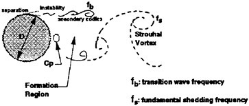
Figure 1: Large-Scale Physics of the Cylinder Near Wake.
The present paper will also discuss LES results of the turbulent wake motion resulting from trailing edge separation of the boundary layer of a NACA 0018 hydrofoil. The US Navy began utilizing the symmetric NACA 0018 section in 1970 to serve as their submarine control surfaces. This particular section as well as other symmetric thick sections can deliver high lift and low drag while maintaining strong structural integrity during complicated maneuvers. Thus, understanding both the instantaneous and mean character of the associated flow at various upstream conditions is crucial for effective use of these sections.
This material is the first in-depth numerical investigation of the fine-scale physics of the NACA 0018 section. The results were generated for upstream velocities at zero angle-of-attack. Previous numerical studies, notably by Hodge et al. (1978) and Sugavanam and Wu, (1980) (among others), used various phenomenological models to represent all the turbulent scales, thus their results can not provide useful details of the fine-scale physics.
To adequately resolve the turbulent wake flow of the cylinder and hydrofoil geometries, nonorthogonal O-type and C-type grid topologies were generated to facilitate control over the spatial resolution. The corresponding LES governing equations were solved in a generalized curvilinear coordinate framework. The dynamic SGS model of Germano et al. (1991) was reformulated for application to the curvilinear space. Since nonorthogonal topologies are often necessary to properly resolve the flow characteristics in many complex domains like these wake flows, the present formulation has extensive applicability.
2. FORMULATION AND NUMERICAL METHOD
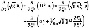
To derive a LES system applicable for complex domains, we begin with the Cartesian form comprised of the continuity and the Navier-Stokes equations. Extension of this coupled system to nonorthogonal grid topologies requires two operations; the transformation phase and the filtering phase. In the following approach, the initial system will be transformed prior to its filtering. This order-of-operations is chosen to facilitate the filter operation which should be administered along the curvilinear grid lines. The filter operates on both the flow quantity and the metric coefficient. Depicting the metric coefficients as filtered is justified herein because the finite-difference expressions used for approximating each metric coefficient are themselves separate mechanisms of spatial filtering. For the present, we will assume that the filter width and local grid spacing are equal; thus, the resolved and filtered turbulent fields are mathematically the same. The LES governing equations appear as
(1)
(2)
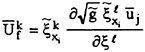
where each term is shown in its non-dimensional strong conservation-law form. The convective term is defined in terms of the resolvable contravariant velocity components ![]()
![]() . The coefficients
. The coefficients ![]() and
and ![]() denote the filtered metrics and the filtered Jacobian of the transformation, respectively. Under this derivation, the subgrid scale (SGS) stress tensor
denote the filtered metrics and the filtered Jacobian of the transformation, respectively. Under this derivation, the subgrid scale (SGS) stress tensor ![]() is defined as
is defined as ![]() .
.
To resolve the cylinder and hydrofoil wake flows, the above LES system was time-advanced by a variant of the fractional-step method (Jordan and Ragab, 1996). Third-order upwind-biased differences approximate the convective derivatives in the wake streamwise and transverse directions. The periodic spanwise components are approximated by a fourth-order accurate compact scheme. A Runge-Kutta procedure is used to time-advance the flow because of its strong numerical stability even under inviscid conditions. The viscous terms are time-split by the Crank-Nicolson scheme and spatially approximated by conservative finite-volume differences. The overall accuracy of the solutions are second order in both space and time. Through extensive testing of this fractional-step method for the wake flows, an error tolerance (residual) of 10−4 was found to be acceptable for terminating convergence of the pressure-Poisson equation. Under this criteria, incompressibility was reached usually in less than 100 iterations at each time increment. Further details of the solution methodology, along with several test cases, can be found in Jordan (1996) or Jordan and Ragab (1996).
3. DYNAMIC SUBGRID SCALE MODEL
The SGS field was modeled by Smagorinsky’s eddy viscosity relationship (Smagorinsky, 1963) and subsequently modified according to Germano et al. (1991) for dynamic computation of the model coefficient. This model gives the correct asymptotic behavior of the turbulent stresses when approaching solid walls and can suitably distinguish between laminar and turbulent flow regimes. For the present application, the SGS model was transformed to the computational space. The curvilinear form of the dynamic model appears as (Jordan and Ragab, 1998)
(3)
where C is considered as Smagorinsky’s coefficient and the filtered metric term ![]() is defined as
is defined as ![]() . In this model, the turbulent eddy viscosity is defined as
. In this model, the turbulent eddy viscosity is defined as ![]() where
where ![]()
![]() and
and ![]() is the grid-filter width. The filtered strain-rate tensor
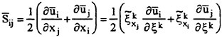
is the grid-filter width. The filtered strain-rate tensor ![]() is defined by
is defined by
(4)
The contravariant form of the resolvable strain-rate field ![]() can be expressed as
can be expressed as ![]() . By combining this transformation with equation (4), the complete definition of the tensor
. By combining this transformation with equation (4), the complete definition of the tensor ![]() is
is
(5a)
(5b)
The first term in equation (5a) is a direct contribution of the CDM to the transformed molecular diffusion term in equation (1), whereas the second term represents the contravariant components of the cell flux vector gradients. To maintain second-order accuracy in time, the Crank-Nicolson and Adams-Bashforth schemes were applied to the first and second components of the total viscous term, respectively.
4. MODEL COEFFICIENT
Smagorinsky’s coefficient in the CDM was acquired by implementing the procedures of Germano et al. (1991) and Lilly (1992). The governing LES equations in curvilinear coordinates were filtered a second time (by a test filter). This third operation gave two resolvable tensors; a modified Reynolds stress tensor ![]()
(6)
and a modified Leonard tensor ![]()
(7)
The second overbar indicates the test filter operation. In both these tensors, the components are computed by test filtering the Cartesian and the contravariant velocity components of the resolved field. As a result, an identity for the Leonard term arises that is defined as ![]() . Modeling the Reynolds stress tensor
. Modeling the Reynolds stress tensor ![]() as
as
(8)
and subsequently using the identity for the Leonard term,
(9a)
(9b)
completes the SGS model definition in curvilinear coordinates. The filter width ratio is defined ![]() . Following the procedure of Lilly (1992), the CDM coefficient can be computed uniquely as
. Following the procedure of Lilly (1992), the CDM coefficient can be computed uniquely as
(10)
This model coefficient can yield both positive and negative values which depict forward and back scatter along the energy cascade, respectively. To inhibit the potential for diverging solutions, backscatter effects of the CDM were truncated to zero in the present applications. Also, a filter width ratio of α=2 was used based on the numerical testing reported by Jordan (1996). Finally, all explicit filtering in the wake simulations were conducted in the computational space using a box-type filter.
5. RESULTS AND DISCUSSION
The present LES investigations focus on the turbulent wake statistics of a circular cylinder and a NACA 0018 hydrofoil. Reynolds numbers for the cylinder and hydrofoil were Re=5,600 and Re=35,000 based on the diameter and cord length, respectively. In both simulations, the flow was impulsively started with unit velocity, zero reference pressure and a fixed non-dimensional time step. Once the lift and drag profiles indicated initiation of the shedding process,new velocity and pressure conditions were imposed along the exit flow boundary. The formulated exit conditions were transformed forms of the continuity and Euler equations, which were found to be satisfactory to exit the shed vortices. An associated exit pressure gradient was computed via the velocity update equation of the fractional-step method to serve as a Neuman boundary condition for the pressure field solution.
5.1 Circular Cylinder
The structured grid for the cylinder test case, shown in Fig. 2, was 241×241×32 (x,y,z directions). While the inflow and outflow outer boundaries were established at 10 and 20 diameters, respectively, the inner no-slip boundary represented the cylinder periphery (s). Along the periphery, the distribution of points was ![]() within the upstream
within the upstream
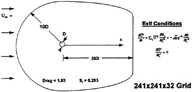
Figure 2: Geometric and Flow Conditions of the Cylinder Near Wake at Re=5,600.
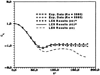
Figure 3. Comparison of the Computed Mean Pressure Coefficient to the Experimental Results of Norberg (1992); (3D)16 Depicts 16 Spanwise Points over Length π and (3D)32 Denotes 32 Points over Spanwise Length 2/3π.
laminar boundary layer and ![]() in the immediate formation region. To insure adequate resolution of the turbulent wall layers (
in the immediate formation region. To insure adequate resolution of the turbulent wall layers (![]() for the first point), all circumferential lines were clustered toward the cylinder surface. The spanwise spacing was
for the first point), all circumferential lines were clustered toward the cylinder surface. The spanwise spacing was ![]() based on the empirical relationship λz/D~20Re−1/2 for the scale (λz) of the large eddies. Finally, the spanwise end conditions were treated as periodic.
based on the empirical relationship λz/D~20Re−1/2 for the scale (λz) of the large eddies. Finally, the spanwise end conditions were treated as periodic.
The base pressure coefficient ![]() is an important parameter to properly resolve because it correlates strongly with the formation length, Strouhal number and strength of the primary vortices. Evidence indicating its numerical accuracy in the present simulation is illustrated in Fig. 3; (Cp)b was time-averaged over six shedding cycles.
is an important parameter to properly resolve because it correlates strongly with the formation length, Strouhal number and strength of the primary vortices. Evidence indicating its numerical accuracy in the present simulation is illustrated in Fig. 3; (Cp)b was time-averaged over six shedding cycles.
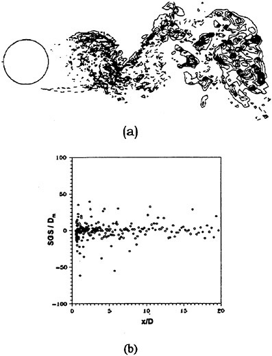
Figure 4. Phase-averaged SGS Model Results; (a) νT/ν Contours, Max. 0.2, Min. −0.2, and Incr. 0.02, (b) SGS/Dm through Wake Centerline.
LES results using only 16 points over spanwise length π as well as a 2D computation clearly illustrate the gross errors attained after separation when the three-dimensionality of the wake flow is ignored or the grid contains a poor spanwise resolution. With 32 points, the drag coefficient averaged to approximately <CD>=1.01 which is within 2 percent of the experimental value found in White (1974)
Before presenting the LES results of the near wake region, questions regarding significant contributions from SGS model must be addressed relative to the inherent artificial dissipation produced when using third-order upwind-biased differences. To appreciate the model’s quality, the investigation should be local. Figure 4 shows phase-averaged results with homogeneity assumed in the spanwise direction. The νT contours (scaled by ν) illustrate negligible contributions in the laminar flow regions and in the wake formation region where the grid
resolution is the highest. Throughout the near wake, nearly 10 percent of the values are greater than 0.1 with approximately 6 percent being positive. Streamwise contributions (SGS)u along the wake centerline (scaled by Dm) suggest a dominant role played by the model locally in regions of high strain-rate activity. Like the vT contours, only slightly more than one-half of these scaled terms were positive.
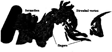
Figure 5. Typical Snapshot of the Three-dimensionality of the Cylinder Near Wake; Iso-surfaces of Vorticity Magnitude (ω=2) Revealing Streamwise “Fingers”.
The snapshot in Fig. 5 of the near wake, in terms of the magnitude of vorticity (ω), clearly displays the formation region structure, Strouhal vortices, and the large-scale streamwise structures connecting the alternating shed vortices. The latter elongated filaments have been experimentally viewed and termed as “fingers” (Gerrard, 1978). These intermediate structures of the near wake persist downstream and posses a high degree of streamwise vorticity, but low streamwise velocity. Thus, in terms of the helicity quantity ![]() they are on the same local scale as the adjacent Strouhal vortices which by comparison contain a high degree of spanwise vorticity, but low spanwise velocity. Each finger is comprised of a pair of counter-rotating vortices with spanwise separation lengths of approximately one diameter (Bays-Muchmore and Ahmed, 1993).
they are on the same local scale as the adjacent Strouhal vortices which by comparison contain a high degree of spanwise vorticity, but low spanwise velocity. Each finger is comprised of a pair of counter-rotating vortices with spanwise separation lengths of approximately one diameter (Bays-Muchmore and Ahmed, 1993).
Past experimental observations and measurements conclude that the most fundamental physics of Strouhal vortices originate from the formation region. The turbulent statistics of that region (time-averaged over six shedding cycles and spatially averaged in the spanwise direction) are plotted in Fig. 6 in terms of the normalized total
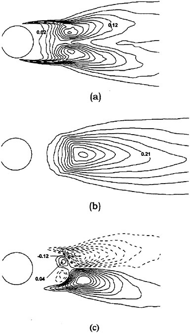
Figure 6. Reynolds Stress Statistics within the Formation Region; (a) ![]() Contour Max. 0.2. Incr. 0.02, (b)
Contour Max. 0.2. Incr. 0.02, (b) ![]() Contour Max. 0.42, Incr. 0.042 and (c)
Contour Max. 0.42, Incr. 0.042 and (c) ![]() Contour Max. 0.12, Min. −0.12, Incr. 0.012. Contours Time-averaged over Six Shedding Cycles.
Contour Max. 0.12, Min. −0.12, Incr. 0.012. Contours Time-averaged over Six Shedding Cycles.
Reynolds stresses ![]() and
and ![]() are the periodic and random components, respectively. The figure shows negligible levels of total stress within the upstream laminar regimes and along the cylinder periphery. Within the separated shear layers, the sharp streamwise contours trace the path leading to final formation of the Strouhal vortices. All three stress components share similar orders of magnitude with their maximums reached near the
are the periodic and random components, respectively. The figure shows negligible levels of total stress within the upstream laminar regimes and along the cylinder periphery. Within the separated shear layers, the sharp streamwise contours trace the path leading to final formation of the Strouhal vortices. All three stress components share similar orders of magnitude with their maximums reached near the
downstream closure limit of the formation region. However, their regional distributions distinctly differ.
Quantitatively, the present total Reynolds stress results agree with the summed periodic and random data reported in Cantwell and Coles (1983) for Re=140,000. Moreover, these results agree with the numerical data at Re=525 (Mittal and Balachandar, 1995), Re=2,600 (Prasad and Williamson, 1997), Re=3,400 (Jordan, 1996) and Re=3,900 (Beaudan and Moin, 1994) which extends similarity of the turbulent stress statistics over the sub-critical range 525≤Re≤140,000. Although the peak magnitudes of each stress at the various Reynolds numbers (listed in Table 1) share similar orders, their respective downstream locations vary. Most importantly, their peak locations correlate well with (Cp)b like the global wake properties discussed earlier (see Fig. 7).
Table 1. Peak Normal and Shear Reynolds Total Stresses within the Formation Region.
|
Total Stress |
Reynolds Number |
||||
|
5251 |
34002 |
39003 |
56004 |
1400005 |
|
|
|
0.21 |
0.17 |
0.18 |
0.20 |
0.22 |
|
|
0.60 |
0.35 |
0.40 |
0.42 |
0.43 |
|
|
0.15 |
0.10 |
0.12 |
0.12 |
0.19 |
|
1Mittal and Balachandar (1995) 2Jordan (1996), 3Beaudan and Moin (1994) 4Present Simulation 5Cantwell and Coles, (1983). |
|||||
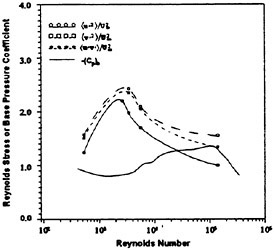
Figure 7. Downstream Location (referenced to cylinder centerline) of Peak Reynolds Stresses and Base Pressure Coefficient as a Function of Reynolds Number (refer to Table 1 for the reference source of the data points).
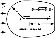
Figure 8. Final Grid Used for the ΝACA 0018 Hydrofoil Simulation.
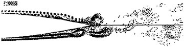
Figure 9. Typical Snapshot of the Vortex Shedding Near the Trailing Edge Tip.
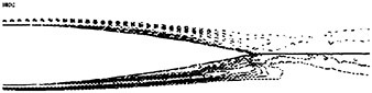
Figure 10. Time-Averaged Vorticity Contours Near the Trailing Edge Tip.
5.2 NACA 0018 Hydrofoil
The grid structure generated for the hydrofoil section was 449×101×16 in the streamwise, transverse and spanwise directions, respectively (see Fig. 8). The inflow and outflow boundaries were set at 4 and 7 cord lengths, respectively. This outflow boundary was established through comparisons to the potential flow solution of the pressure variable along the section surface. Like the cylinder test case, the field lines were cluster towards the hydrofoil section to insure a minimum boundary condition in wall units of Δy+<4 normal to the surface. The spanwise length was set at π units with periodic end conditions.
The periodic shedding of vortex structures off the trailing edge of the NACA 0018 hydrofoil are shown in Fig. 9. The contours depict instantaneous
vorticity with homogeneity assumed in the spanwise direction. The vortical structures rapidly traverse the trailing edge of the hydrofoil with subsequent shedding near the tip. In the immediate wake region, successive vortices closely interact such that their mutual interference causes breakdown or pairing. These observations were also detected in the flow visualization tests reported by Hayashi et al. (1995). Notably, this behavior is particularly unlike the vortex shedding process of a cylinder discussed above where the shed vortices are a several diameters apart and remain strongly coherent for many diameters downstream of formation.
The spanwise vortical structures traverse along the trailing edge and their associated shedding statistics are not as well-understood as the vortex formation process behind a circular cylinder. The time-averaged vorticity contours shown in Fig. 10 suggest a fully attached boundary layer. Only extremely close to the hydrofoil surface (over a few grid spaces) does the mean vorticity contours indicate pockets of minor circulation. Since the instantaneous separation point strongly oscillates near the maximum hydrofoil thickness, its defined time-averaged location appears absent.
Spanwise-averaged profiles of the total lift (CL) and total drag (CD) are plotted in Fig. 11 over approximately eight shedding cycles. The lift profile depicts minor fine-scale oscillations which suggests little sign of turbulent activity or even transition to turbulence along the trailing edge. While the mean drag coefficient is approximately 0.035, the net lift coefficient is 0.18. Based on the hydrofoil thickness (t), the lift profile gives a Strouhal number (St=f·t/U∞) of 0.18 which compares favorably with 0.19 as measured by Hayashi et al. (1995) and 0.21 as numerically predicted by Hodge et al. (1978) at zero angle-of-attack..
The time-averaged pressure coefficient (Cp) in Fig. 12 is compared to the computational results at Re=41,400 as reported by Thompson et al. (1976) for a fully-attached steady laminar boundary layer. The disparity between the pressure and suction sides agrees with the net lift coefficient given above by the total lift profile. The dash line in the figure depicts results obtained if the flow is assumed to be inviscid.
Discernible turbulent activity of the NACA 0018 hydrofoil at Re=35,000 is confined primarily to the trailing edge tip as illustrated in Fig. 13. Contours
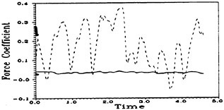
Figure 11. Profiles of Total Lift and Drag Coefficient Over 7 Shedding Cycles.
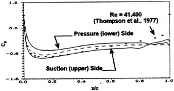
Figure 12. Profiles of the Pressure Coefficient Over 7 Shedding Cycles.
of the horizontal turbulent intensities ![]() are shown in Fig. 13a while the shear components
are shown in Fig. 13a while the shear components ![]() are depicted in Fig. 13b. Further downstream in the near wake region as well as along the trailing edge, some turbulent activity is indicated but their levels are extremely low. Thus, although the trailing flow has massively separated it remains essentially laminar over a majority of the trailing edge at this Re.
are depicted in Fig. 13b. Further downstream in the near wake region as well as along the trailing edge, some turbulent activity is indicated but their levels are extremely low. Thus, although the trailing flow has massively separated it remains essentially laminar over a majority of the trailing edge at this Re.
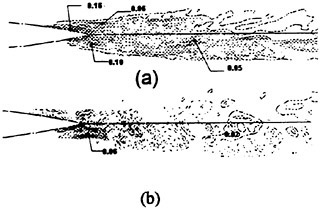
Figure 13. Contours of Reynolds Stresses; (a) Streamwise, (b) Shear
6. FINAL REMARKS
The impetus of the present large-eddy simulations was to investigate the turbulent physics of the near wake behind a circular cylinder and a NACA 0018 hydrofoil. The governing LES equations and subgrid-scale (SGS) turbulence model were formulated in curvilinear coordinates by performing the transformation operation of the full-scale resolution equations prior to their filtering.
The LES investigation of the circular cylinder extends our understanding of the wake physics and provides useful analyses for engineering design. We know that the streamwise “fingered” structures and spanwise vortical structures appear to scale according to the helicity. Also, the Reynolds stress statistics share equivalent orders-of-magnitude and similar distributions over the entire range of sub-critical Reynolds numbers. Finally, the location of the peak Reynolds stresses within the formation region scale according to the magnitude of the downstream base pressure coefficient.
With the exception of the trailing edge tip region, the flow is primarily laminar at this Re. The flow separates just after the maximum thickness of the section thereby generating large-scale separation bubbles which transverse the trailing edge. Within the near wake, these large-scale structures interact and eventually pair or apparently breakdown. They do not remain coherent far downstream. Significant turbulent characteristics are confined to a region surrounding the trailing edge tip. Relative to the mean flow, peak intensities are generally under 10 percent.
ACKNOWLEDGMENTS
The author gratefully acknowledges the support of the Office of Naval Research (Dr. L.P. Purtell, Scientific Officer), Contract No. N0001497-WX20346 and the In-house Laboratory Independent Research Program (Dr. S.Dickinson, Coordinator) at the Naval Undersea Warfare Center Division Newport.
REFERENCES
1. Bays-Muchmore, B. and Ahmed, A., (1993), “On Streamwise Vortices in Turbulent Wakes of Cylinders,” Physics of Fluids, A. 5, pp. 387–392.
2. Beaudan, P. and Moin, P., (1994), “Numerical Experiments on the Flow Past a Circular Cylinder a Sub-Critical Reynolds Number,” Report No. TF-62, Stanford University, Stanford, CA.
3. Cantwell, B. and Coles, D., (1983), “An Experimental Study of Entrainment and Transport in the Turbulent Near Wake of a Circular Cylinder,” Journal of Fluid Mechanics, Vol. 136, pp. 321–374.
4. Germano, M., Piomelli, U., Moin, P., and Cabot W.H., (1991), “A Dynamic Subgrid-Scale Eddy Viscosity Model,” Physics of Fluids, A. 3, pp. 1760–1765.
5. Gerrard, J.H., “The Wakes of Cylindrical Bluff Bodies at Low Reynolds Number,” Phil. Transactions Royal Society of London, Vol. 288, pp. 351–382.
6. Hayashi, H., Kodama, Y., Fukano, T. and Ikeda, M., (1995), ‘Relation between Wake Vortex Formation and Discrete Frequency Noise,’ Separated and Complex Flows, FED-Vol. 217, pp. 107–114.
7. Hodge, J.K., Stone, A.L. and Miller, T.E., (1978), “Numerical Solution for Airfoils Near Stall in Optimized Boundary-fitted Curvilinear Coordinates,” AIAA, Vol. 17, No. 5, pp. 458–464.
8. Jordan, S.A., (1996), ‘A Large-Eddy Simulation Methodology for Incompressible Flows in Complex Domains,’ NUWC-NPT Technical Report 10, 592.
9. Jordan, S.A. and Ragab, S.A., (1996), “An Efficient Fractional-Step Technique for Unsteady Three-Dimensional Flows,” Journal of Computational Physics, Vol. 127, pp. 218–225.
10. Jordan, S.A. and Ragab, S.A., (1998), “A Large-Eddy Simulation of the Near Wake of a Circular Cylinder,” Journal of Fluids Engineering, (to appear).
11. Kato, C., Iida, A., Takano, Y. Fujita, H. and Ikegawa, M., (1993), “Numerical Prediction of Aerodynamic Noise Radiated from Low Mach Number Turbulent Wake,” AIAA 93–0145.
12. Lilly, D.K., (1992), “A Proposed Modification of the Germano Subgrid-Scale Closure Method,” Physics of Fluids, A. 4, pp. 633–635.
13. Mittal, R. and Moin, P. (1997), “Suitability of Upwind-Biased Finite Difference Schemes for Large-Eddy Simulation of Turbulent Flows”, AIAA Journal, Vol 35, No. 8, pp. 1415–1417.
14. Mittal, R. and Balachandar, S. (1996), “Effect of Three-dimensionality on the Lift and Drag of Nominally Two-dimensional Cylinders”, Physics of Fluids, Vol 7, No. 8, pp. 1841–1865.
15. Prasad, A. and Williamson, C.H.K., (1997), “Three-Dimensional Effects in Turbulent Bluff-Body Wakes,” Journal of Fluid Mechanics, Vol. 343, pp. 235–265.
16. Smagorinsky, J., (1963), “General Circulation Experiments with the Primitive Equations, I. The Basic Experiment,” Monthy Weather Review, Vol. 91, pp. 99–164.
17. Sugavanam A. and Wu, J.C., (1980), “Numerical Study of Separated Turbulent Flow over Airfoils,” AIAA, Vol. 20, No. 4, pp. 464–470.
18. Thompson, J.F., Thames, F.C., Hodge, S., Shanks, S.P., Reddy, R.N. and Mastin, C.W., (1976), ‘Solutions of the Navier-Stokes Equations in Various Flow Regimes on Fields Containing and Number of Arbitrary Bodies Using Boundary-fitted Coordinates Systems, 5th International conference on Numerical Methods in Fluid Dynamics, Euschede, Netherlands
19. White, F.W., (1974), Viscous Fluid Flow, McGraw-Hill, NY.
20. Zhou Y. and Antonia, R.A., (1993), “A Study of Turbulent Vortices in the Near Wake of a Cylinder,” Journal of Fluid Mechanics, Vol. 253, pp. 643–661.
DISCUSSION
J.Grant
Naval Undersea Warfare Center, USA
This paper is an important contribution to the computation of complex flows. The author begins by providing a clear description of the form of the filtered equations in the context of a body-fitted coordinate system, including the formulation of the dynamic subgrid scale model. The two cases presented, flow past a right circular cylinder (Re=5600) and flow past a NACA 0018 hydrofoil (Re=35000), are among the most complex yet reported in the literature.
The computed pressure distribution for the former case compares well with measurements made at similar Reynolds numbers, indicating that the separation point was accurately depicted by the computations. The computed pressure distribution for the hydrofoil displays a similarly good agreement with relevant experimental results.
The spatial distributions shown in Figure 6 of the phase-averaged Reynolds stresses will be useful for understanding the momentum budget for the cylinder wake vortices in the formation region. The results reported in Table 1 and Figure 7 concerning the magnitude and location of maxima suggest that the spatial distribution plots are reasonably quantitatively accurate; comparison of cross-wake profiles of the stresses with observed data would strengthen this point. Although the stated focus of this paper is on the turbulent statistics, a plot of computed and measured cross-wake variation of the mean flow would be a useful supplement to the displayed results.
There is quite a bit of ongoing discussion in the literature concerning the impact of numerical error on the results of LES calculations, and the author could have used this paper as an opportunity for contribution to this subject. First, a plot in the format of Figure 4 (a) showing contours of the ratio of truncation error for the advection term to the magnitude of the viscous term would be very helpful in understanding the relative roles of the subgrid scale model and numerical viscosity, especially as the grid spacing increases away from the cylinder. (Truncation error could be estimated by computing the leading term.) Second, a plot of the spectrum of the kinetic energy showing the roll-off—or lack of roll-off—at the higher resolved wavenumbers would further comment on this issue.
Overall, this paper displays the impressive potential for subgrid scale modeling to compute complex unsteady flows at relevant Reynolds numbers.
AUTHOR’S REPLY
First of all, I would like to thank Dr. Grant for expressing his appreciation of the paper. It does indeed present useful information regarding the Reynolds stress fields downstream of a circular cylinder and a NACA 0018 hydrofoil. I am currently focused on the cross-wake statistics downstream of these shapes, as recommended by Dr. Grant, and hope to publish the respective LES results at the next Navy symposium.
As noted by Dr. Grant, the accuracy of the convective term and its instantaneous as well as statistical interaction with the SGS term is crucial to any LES computation. The associated
metric coefficients which accompany the transformation operation should be evaluated numerically to at least fourth-order. Choice for evaluating the derivative itself, however, depends largely on treatment of the GS stress field.
For example, contributions of a Leonard-type term are negligible at the higher resolved wavenumbers if one chooses to discretize the convective term to the second-order. One can understand this fact by comparing the energy spectrum of a box-filtered field to that of the corresponding Leonard-term. In the present paper, a third-order upwind biased scheme was combined with the dynamic model which represented the turbulent scales unresolved by the grid spacing. Although previously shown by others, severe damping, or even dumping, of turbulent energy at the higher resolved scales did not occur under the present grid resolution. This observation is evident by the close comparisons attained between the LES and experimental data (see Jordan and Ragab, 1998).
To address the truncation error issue, Table 1 lists the relative contributions of the convective, diffusive, SGS, truncation error and artificial dissipative terms in the computations of the cylinder wake. These values depict time-averages taken within the turbulent wake region over approximately 8 shedding cycles. Clearly the wake dynamics are dominated by convection. For the present spatial resolution, the SGS term contributes on the order of the diffusion term. This fact is further emphasized in Figure 1, which shows the instantaneous scaled turbulent eddy viscosity along the wake centerline taken at a particular instant in time.
Table 1: Phase-averaged Terms (Re=5,600); Convection (Cv), Molecular Diffusion (Dm), Subgrid Scale Stress (SGS), Truncation Error (TE) and Artificial Dissipation (Da)
|
Cv |
Dm |
SGS |
TE |
Da |
|
O(1) |
O(10−1) |
O(10−1) |
O(10−2) |
O(10–2) |
|
|
||||
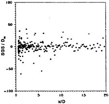
Figure 1. Phase-averaged SGS Model Results; SGS/Dm through Wake Centerline.
One can conclude from these results that the SGS term does indeed participate in the LES computations of the cylinder wake flow, but generally on the order of the diffusion term. Under-prediction of the Reynolds stress statistics in the coarse-grid regions is directly attributed to the inability of the SGS model to accurately account for the turbulent scales that encompass the inertial sub-range and dissipative range of the energy spectrum.
Reference
Jordan, S.A. and Ragab, S.A. (1998), “A Large-Eddy Simulation of the Near Wake of a Circular Cylinder,” Journal of Fluids Engineering, V120, No. 2, pp. 243–252.
Resistance in Unsteady Flow: Search for a Physics-Based Model
T.Sarpkaya (Naval Postgraduate School, USA)
ABSTRACT
This paper addresses the old and difficult problem of devising a physics-based model for the prediction of flow-induced unsteady forces acting on bluff bodies immersed in relatively more manageable time-dependent flows. The modification proposed herein to the existing MOJS (1) equation through the addition of a third term is expected to offer greater universality and higher engineering reliability, particularly in the so-called drag-inertia regime.
INTRODUCTION
Unsteady flows over bluff bodies arise in many engineering situations and the prediction of the fluid/structure interaction (forces and dynamic response) presents monumental mathematical, numerical and experimental challenges (2–7).
Numerous formulations of the force exerted on a rigid body moving in translational motion in a viscous fluid have been derived which require either the velocity or the vorticity field to be known throughout the whole fluid space [see, e.g., Howe (8) and Lighthill (9)]. Howe (8) has shown that the force Fi exerted by the fluid on a rigid body in the i-direction is given by
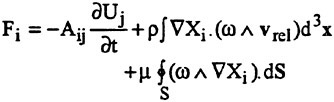
(1)
in which Aij is the added mass tensor of the body for translational motion, vrel (=v−U) is the relative velocity, Xi is the velocity potential of the irrotational flow about the body, dS is the elemental surface area, and w is the vorticity. It is seen that Fi is represented as the sum of its three constituent components: An inviscid inertial force, vector sum of the normal surface stresses induced by vorticity in the fluid, and the shear force or skin friction. Neither the above decomposition nor the interpretation of the resulting elements is unique. In fact, Fi could have been decomposed into a smaller or larger number of components, with each term acquiring a new meaning. For example, Lighthill (9) expressed the force F in terms of the moment of the vorticity distribution over the entire space, as
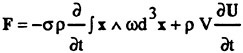
(2)
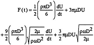
where s=1/2 for three-dimensional flows and V is the volume of the body. According to Eq, (2), the first term represents the total contribution of vorticity and the second term the inviscid inertial force. Unfortunately, only under rare circumstances that the velocity or the vorticity field is known throughout the whole fluid space. Two canonical laminar flow examples are given by Stokes (10). He presented the solutions for both a cylinder and a sphere oscillating in a liquid with the velocity U=−Aωcosωt, assuming that the amplitude A of oscillations is small and the flow about the bodies is laminar, unseparated, and stable. For a sphere, his solution may be written as,
(3)
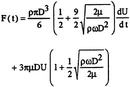
in which the first term on the right-hand side represents the added-mass (its ideal value) times acceleration; second term, the linear viscous resistance to the steady motion of a sphere at very low Reynolds numbers (say, Re<1); the third term, either the effect of history of the motion on the inertial force or simply the viscous effects in harmonic motion on the acceleration-dependent forces; and the last term, the history effect on the linear drag. Also, one may combine the last two terms and regard them as history-dependent modifications to the ideal values of the inertia and drag forces. Equation (3) may be further rearranged as,
(4)
where the force is composed of two parts: an inertial force and a drag force, linearly dependent on acceleration and velocity and modified by the bracketed coefficients, dependent on (πβ)−1 and (πβ), respectively, where β=fD2/v with f=ω/2π. In other words, one may state that the generation, convection and diffusion of vorticity affect not only the skin friction and form drag, but also the inertial force. In fact, it will be shown later that the rate of change of the kinetic energy associated with the motion of the shed vorticity modifies both the drag and the inviscid inertial force.
Stokes solution (10) for a circular cylinder may be written as
(5)
in which Ca is the added mass coefficient, expressed in terms of the displaced mass M'=(πρR2), and C' is a damping coefficient, since the second part of the equation, namely −C'M'Uoω coswt, is out of phase with the acceleration and opposes the motion of the body. Both of these coefficients depend on β since the motion is controlled by the viscous as well as the pressure forces. In inviscid fluids, only the latter is present and Ca=1 for a circular cylinder and Ca=0.5 for a sphere.
The coefficients Ca and C' decrease with increasing β. In fact, for a cylinder, for large values of β, one has
(6)
and
(7)
Wang (11) extended Stokes analysis to Ο[(πβ)−3/2] using the method of inner and outer expansions. His solution, valid for A/D≪1 and b ≫1, for stable, unseparated laminar flow oscillating sinusoidally about a cylinder, may be reduced to
(8a)
and
(8b)
which may be compared with Eqs. (6) and (7). The results differ only in the last terms and yield virtually identical results in the range of their validity. Once again it is clear that both the inertia and damping coefficients are modified by β, at least in sinusoidally oscillating unseparated flow.
Stokes classical solutions (10) formed the basis of many subsequent models where the oscillations are presumed to be small enough to allow convective accelerations to be ignored. An extensive review of the existing force models has shown that the degree of empiricism increases with increasing Reynolds number and some measure of the unsteadiness of the motion. The practice of expressing the time-dependent fluid force as a function of the prevailing velocities and accelerations has been extended to nonlinear motions where convective accelerations, separation, and three-dimensional wakes are important. Some of these efforts expressed the force as a sum of the quasi-steady component (a function of the body shape and the instantaneous Reynolds number), an ideal inertia component, and a history expression [first noted by Basset (12)]. These efforts, reaching to recent times, often produced awkward expressions, applicable to a very narrow class of motions (13). This was due to the complexity of the problem rather than due to the lack of imagination of the model makers. Even in a sinusoidally oscillating flow (a relatively more manageable unsteady flow), every Re (Reynolds number=UmD/v), Kc (Keulegan-Carpenter number=UmT/D=2πΑ/D), and k/D (relative sand roughness) combination represents a unique flow situation. As yet a theoretical analysis of the problem for separated flow is difficult and much of the desired information
must be obtained experimentally and, if possible, numerically.
The computational representation of a turbulent motion, without proper physics, is a major roadblock to the ultimate promises of the CFD. Equally important is the fact that in highly complex, separated, time-dependent turbulent flows with large-scale unsteadiness about small bodies (with negligible diffraction effects), such as those considered herein, the Reynolds number varies between zero and a desired maximum during a given cycle and the flow is three dimensional (2-D flows and 2-D turbulence exist only in thought experiments). Even if one were to develop validated, rationally-constructed, two- or higher-order-equation turbulence models, there is no assurance that they will yield reliable results for time-dependent flows. Therein lies the difficulty of the numerical simulation of unsteady non-equilibrium turbulent flows, with or without separation. As it stands, the state of the art is less than satisfactory not only because of the limitations of computational resources and the lack of understanding of the physics of turbulence, but also because the real-time control applications (remotely operated vehicles; multiple-link, multi-degree-of-freedom, underwater manipulators) demand hydrodynamic forces and torques in real time as a function of the state and state derivatives of the system.
The control of unsteady vehicle motions cannot, by their very nature, wait for day-long computer solutions or for the improvement of the current state of the computational an through the use of quantum computers. To make matters worse, the motions of underwater manipulators are often short enough to occur in transient, rather than in quasi-steady states. Thus, the intelligent control of such vehicles requires the determination of the forces and torques predominantly during these transient states. This is a very demanding challenge to experimental and computational fluid dynamics communities and points out the necessity of parallel studies, in the years to come, for the pursuit of demonstrably sound semi-empirical approaches [perhaps something better than the MOJS1 (1) equation] for the prediction and execution of minimum-time or minimum-energy trajectories in complex environments. In this respect, the experimental studies of Morison, O’Brien, Johnson, and Schaaf (MOJS) on the forces on piles due to the action of progressive waves have provided a useful, somewhat heuristic, and so far irreplaceable approximation.
THE MOJS EQUATION
In a paper submitted to the Petroleum Transactions of AIME on 23 October 1949, Morison, O’Brien, Johnson, and Schaaf (1950) (referred to hereafter as MOJS) wrote: “The force exerted by unbroken surface waves on a cylindrical object, such as a pile, which extends from the bottom upward above the wave crest, is made up of two components, namely: (1) A drag force proportional to the square of the velocity which may be represented by a drag coefficient having substantially the same value as for steady flow, and (2) A virtual mass force proportional to the horizontal component of the accelerative force exerted on the mass of water displaced by the pile. These relationships follow directly from wave theory and have been confirmed by measurements…” Thus was born the MOJS equation:
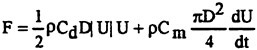
(9)
where F is the force per unit length experienced by a cylinder, D is the characteristic dimension, U and dU/dt represent the undisturbed velocity and the acceleration of the fluid at the axis of the small body, and Cd and Cm are the Fourier- or Least-Squares-Averaged drag and inertia coefficients.
Equation (9) does not deal with the transverse force. Its numerous limitations and inadequacies, partly associated with the wake reversal and partly with the creation, convection, and transverse arrangement of vortices, have been repeated almost ad nauseum (see, e.g., 3, 5, 14–15). However, The experience of the past 50 years has also shown that the MOJS equation still represents the best two-coefficient fit to the measured force. In the so-called drag/inertia regime, it produces relatively poor results where the error (defined, e.g., as the RMS value of
the difference between the measured and predicted forces, normalized by the RMS value of the measured force) may be as large as 50%. The addition of two more terms (a four-term Morison equation) through the introduction of two additional coefficients (dependent on Kc only2), as proposed by Keulegan and Carpenter (16) in their seminal work, does not always improve the predictions of the extended MOJS equation. In fact, in many cases it makes them even worse! Furthermore, it is clear after 50 years of experience with the MOJS equation that the engineering community is not interested with equations with four empirically-determined coefficients (14–15). In fact, if there are no better alternatives to an approximate model whose predictions are correct some of the time and not too far from the truth (measurements) at other times, then one becomes dependent to that approximate model for all times. We are also well aware of the fact that all other alternatives to the MOJS equation may not spark a new storm! In either case, we are reminded by Paul Adrien Maurice Dirac that “A theory with mathematical beauty is more likely to be correct than an ugly one that fits some experimental data.”
In view of the foregoing, at least three additional approaches may be pursued: (i) a full numerical analysis of the problem through the use of DNS, LES, RANS, or FANS, (ii) calculation of forces from the measured vorticity distributions through the use of PIV and/or LDV), and (iii) additional efforts to devise a new force model and/or to improve the MOJS equation. It is becoming increasingly clear that Direct Numerical Simulations (DNS) and/or large Eddy Simulations (LES) only offer a few data points, do not yet deal with high-enough Reynolds numbers and technologically-significant problems, and do not provide real-time information. The prediction of force from vorticity distribution, obtained through the use of the Digital Particle Image Velocimetry (DPIV), (an equally expensive and specialized technique) does not lead to a predictive model, only to the verification of the well-known integral expressions [e.g., Eq. (2)] at a few prescribed times. Thus, one is left with the art of devising relatively simple models with accuracy better than that of the MOJS equation.
The inertia and drag coefficients in the MOJS-model are forced to share the contributions of the vorticity field. Thus, the question naturally arises as to why one should not express the resistance in time dependent flows as a sum of the contributions of (a) an inviscid inertial force (with a precisely determinate inertia coefficient, unlike that in Morison’s equation) and (b) a vorticity-drag (in-line components of skin friction and form drag) due to concentrated and distributed vorticity shed during the entire history of the motion (expressed, if at all possible, in terms of a single coefficient, dependent on Re, Kc, and k/D). In fact, Lighthill (9) asserted that the viscous drag force and the inviscid inertia force operate independently and therefore it is possible to divide the measured time-dependent force into two distinct components: an inviscid inertial force, either corrected or uncorrected for a weakly non linear flow field (19), and a viscous drag force. Lighthilľs assertion is based on Kelvin’s Minimum Energy Theorem which assumes that the motion of the unbounded external fluid may be expressed as a linear sum of (a) the potential flow that satisfies the boundary conditions; and (b) a residual vortex motion which satisfies the zero boundary conditions (at the interface and at infinity).
This led Lighthill (9) to suggest that “…the irrotational part (a) of the fluid motion depends only upon those boundary conditions which it satisfies instantaneously.” “This is the part [unlike (b), the vortex motion] which is devoid of any ‘memory’ for earlier values taken by U(t); rather, it is proportional simply to the current value of U, and its kinetic energy is proportional to U2,…so that 1/2 MaU2 can be thought of as if it were the kinetic energy of an added mass Ma of fluid which the body’s motion effectively drags along with it.” Then he goes on to state that “Simultaneously, the kinetic energy of part (b), the vortex motion, is increasing as more and more vorticity is shed into the wake, where the vortex lines are subsequently convected and diffused. The rate of working by the thrust with which the body acts upon the fluid is necessarily equal to the rate of increase of the total energy of the fluid; including (it must be emphasized) both the kinetic energy of part (b) and any thermal energy into which viscous dissipation may progressively convert that kinetic energy.” However, Lighthill does not associate the increase in kinetic energy of part (b) with any added mass as he has done so with that of part (a) as if the fluid ‘knew’ how to differentiate the two increases in kinetic energy (one due to U and the other due to dU2/dt. In fact he goes on to state that “An estimate of the rate of
increase of energy in part (b) may be derived from the rate, proportional to ρAU (where A is the body’s frontal area), at which the mass of wake fluid is growing. Velocities of the vortex motion are proportional to U, giving a rate of increase of energy (1/2)ρAU2Cd, where Cd is a coefficient. The corresponding thrust required to yield this rate of working, and to overcome the equal and opposite vortex-flow drag of the fluid on the body, is (1/2)ρAU2Cd.” This implies that the drag force is proportional to the square of the instantaneous velocity only, with no effect of the time rate of change of the kinetic energy as if the vorticity field were comprised of inviscid line vortices of constant strength [a detailed discussion of this is given in (4, 20)].
Lighthill (9) re-wrote the MOJS equation as
(10)
which for an ambient flow defined by U(t)=−Umcosωt it reduces to
(11)
where ![]() now is the ideal value of the added mass coefficient and A and V are the projected area and the volume of the body, respectively. Lighthill’s version of the MOJS equation requires only one experimentally determined coefficient: Cd, presumably dependent on such parameters as the Reynolds number, Keulegan-Carpenter number, relative roughness, direction of the body motion. We will now show that it is impossible to find a suitable Cd value which enables Eq. (11) to represent the measured force even for a circular cylinder.
now is the ideal value of the added mass coefficient and A and V are the projected area and the volume of the body, respectively. Lighthill’s version of the MOJS equation requires only one experimentally determined coefficient: Cd, presumably dependent on such parameters as the Reynolds number, Keulegan-Carpenter number, relative roughness, direction of the body motion. We will now show that it is impossible to find a suitable Cd value which enables Eq. (11) to represent the measured force even for a circular cylinder.
Figures 1 and 2 show representative measured forces for a sinusoidally oscillating flow about a circular cylinder. Also shown in these figures are the traces of force calculated using Eq. (11), with a Cd value that makes the maximum measured and calculated forces nearly agree, and the difference between the measured and calculated forces (the residue). These figures as well as several thousand others have shown conclusively that it is impossible to represent the measured force with Eq. (11) regardless of what value one assigns to Cd, as long as ![]() (here equal to 2.0) is used. The form of the residue immediately suggests, as verified by a proper Fourier analysis, that Eq. (11) must be augmented by a term involving sinωt (proportional to the acceleration of the flow). Using the Cd value deduced from a Fourier analysis of the measured force as the most appropriate drag coefficient, one has
(here equal to 2.0) is used. The form of the residue immediately suggests, as verified by a proper Fourier analysis, that Eq. (11) must be augmented by a term involving sinωt (proportional to the acceleration of the flow). Using the Cd value deduced from a Fourier analysis of the measured force as the most appropriate drag coefficient, one has
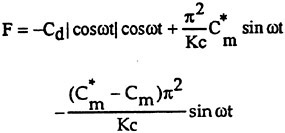
(12)
which is obviously identical to MOJS equation. Here Cm is identical to the inertia coefficient Cm in the original MOJS equation and is obtained in exactly the same manner as before. It must be emphasized that the use of a smaller or larger Cd could not have provided a better fit to the measured force. Furthermore, it would have required additional coefficients resulting from the expansion of Cd into a suitable series.
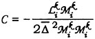
Two additional pieces of information that may be gleaned from Eq. (12). The first is that the coefficient of the last term is indeed an important parameter, designated here by,
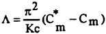
(13)
which has a clear physical meaning. It reflects the modification of the inertial force by the creation, convection, and diffusion of vorticity, as in Eq. (4) of Stokes (10). The second is that the corrections to the MOJS equation are primarily of inertial nature due to the rapid motion of the concentrated vorticity and, to a lesser extent, due to the alterations in the skin-friction and form drag. Thus, the nature of an additional term in the MOJS equation must necessarily involve sin3ωt, with a functional dependence at least on Λ. Previously, as part of a similar effort, Sarpkaya (14–15) used a slightly different parameter, defined by,
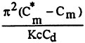
(14)
partly because it approached zero for both small and large values of Kc and partly because it represented the ratio of the deviation of the maximum inertial force from its ideal value to the maximum drag force (for a circular cylinder). The representation of the residue
resulted in a four-term MOJS equation which was rather cumbersome.
The search for a simpler model needed additional inspiration and rules for thought experiments because the form of the next term is not known a priori and is not intuitively obvious. Furthermore, a mere series representation of as many of the remainder terms as possible is not fluid-mechanically satisfying and will serve no useful purpose. The problem is further compounded by the difficulty of accurately measuring the velocities and accelerations and of deciding what values of the two coefficients should be used in the MOJS equation or in its modified version. In general, the nature of the equation rather than the lack of precision of measurements or the difficulty of calculating the kinematic characteristics of the flow from the existing wave theories has been criticized. This may be true in the drag-inertia regime, but certainly not in the region where Kc is larger than about 20. Even in its restricted form the modified MOJS equation may be very useful in design of structures subjected to regular waves and in the analysis of the dynamic response of small bodies for which the diffraction effects are negligible.
Obviously, the purpose of the model maker cannot be to devise a model that covers all circumstances, be that a modified MOJS equation or another turbulence model. That would tantamount to the understanding of the physics of turbulence and having the power to compute any flow situation. We consider neither within the realm of possibility. Thus, a model is based largely on heuristic reasoning, mathematical simplicity, intuition, empirical correlations, constraints imposed by physical realizability, and experimental justification of the predictions. Hopefully, a model having these features should also have the following characteristics: (a) it should address to the most important shortcomings of the MOJS equation; (b) It should apply equally well over all ranges of Kc, Re, and k/D (within the small body constraint); (c) it should have distinct advantages over the MOJS equation; (d) It should not require additional empirical coefficients beyond those already in use (i.e., Cd, Cm, and, of course the lift coefficient); (e) it should be extrapolatable to more complex flow situations (with some poetic license!).
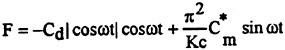
With the following thoughts on mind, extensive efforts during the past eighteen years to find a much simpler parameter, dependent only on the new Λ, as defined by Eq. (13), and Cd have shown that Λ|Λ|/Cd does indeed serve the intended purpose well. We write the modified version of the MOJS equation simply as
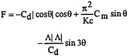
(15)
It has the following attributes: (a) It preserves the simplicity of the original MOJS equation; (b) it reproduces the measured force with remarkable accuracy (the rms value of the residue, normalized by the rms value of the measured force remains less than 10 percent for all smooth and rough cylinder data within the range of Re, Kc, and k/D values encountered in Sarpkaya’s experiments (17–18,21–27), (c) it does not require the evaluation of any new coefficients or look-up tables, and (d) it holds true not only for circular cylinders but also for flat plates.
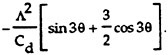
If one wishes even higher accuracy, it can easily be achieved by adding a cos5θ term, as follows
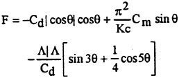
(16)
The additional correction brought about by the cos5q term is negligible as evidenced by sample plots shown in Figs. 3 and 4. We will therefore refer to Eg. (15) as the modified MOJS equation. We will not consider here higher order harmonics partly because they make the model less attractive and partly because their contribution is often negligibly small as seen in our calculations with over 2000 measurements in a broad range of Reynolds numbers, Keulegan-Carpenter numbers, and relative roughnesses. Furthermore, in technological applications, the accuracy of the kinematical input is not, for understandable reasons, commensurate with the additional refinement brought about by the fourth term.3
 The difference between this and the one for a circular cylinder [Eq. (16)] is due to difference in the Strouhal numbers of the two bodies (about 0.21 for the cylinder and about 0.14 for the bluff plate)
RESULTS AND CONCLUSIONS
Extensive calculations for all values of Kc and β (previously encountered by this investigator) have shown that the new model predicts the measured force with an error (noted above) less than 10% in all ranges of the governing parameters. Eight randomly selected force plots are shown in Figs. 5 through 12 for four smooth and four rough cylinders. Each figure contains four curves representing the measured force, the prediction of the MOJS equation, the prediction of the modified MOJS equation (i.e., Eq. 15), and the residue (the predicted force minus the measured force)4
It is clear that Eq. (15) with three terms and only two experimentally determined coefficients (Cd and Cm) predicts the measured force accurately enough even in the so-called drag/inertia dominated regime. At Kc values smaller than about 7 and larger than about 20, the MOJS equation and its modified version predict the measured force with equal accuracy and, in fact, the force traces become indistinguishable. Figures 13 and 16 show four sample plots for a bluff plate. Suffice it to note that Eq. (15) makes a satisfactory representation of the measured force relative to the original MOJS equation.
It may be concluded on the basis of our observations and measurements that the MOJS equation can be suitably modified through the use of a new parameter, defined by (Λ|Λ|/Cd), with 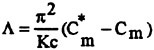 . It has been adopted here primarily for three reasons: Heuristic reasoning when applied to relevant conditions, mathematical simplicity, and the experimental justification of the model.
It has been shown that the viscous drag force and the inviscid inertia force do not operate independently and it is not possible to divide the measured time-dependent force into an inviscid inertial force and a viscous drag force. Our results have shown convincingly that both components of the force are affected by the creation, convection, and diffusion of vorticity. However, the justification of the predictions of a model by one particular set of experimental data is never sufficient. A model is ultimately judged by its prediction of measurements from as many sources as possible. We, therefore, hope that other researchers with reliable experimental data will compare their measurements with the modified MOJS model.
The application of Eq. (15) to the prediction of the in-line response of cylinders, particularly in the drag-inertia dominated regime, will be the subject of another paper.
|
4 |
The sign of the residue helps one to quickly identify which of the two solid curves is the predicted force. |
ACKNOWLEDGMENTS
This investigation has been supported by the Office of Naval Research under contract N0001497WR30013. I am particularly indebted to Dr. Thomas F.Swean, Jr., Code 3201E, Team Leader of the Ocean Engineering and Marine Systems S&T Area, for his continuous guidance and encouragement.
REFERENCES
1. Morison, J.R., O’Brien, M.P., Johnson, J.W., and Schaaf, S.A., “The Forces Exerted by Surface Waves on Piles,” Petroleum Trans., AIME, Vol. 189, 1950, pp. 149–157.
2. Sarpkaya, T., “Brief Reviews of Some Time-Dependent Flows,” J. Fluids Engng. Trans. ASME, Vol. 114, No. 3, 1992, pp. 283–298.
3. Sarpkaya, T., “Forty Years of Fluid Loading—The Past and Beyond,” Proceedings of the International Conference on the Behavior of Offshore Structures, Vol. 1, 1992, pp. 283–293.
4. Sarpkaya, T., “Unsteady Flows,” Chapter 12, in Handbook of Fluid Dynamics and Fluid Machinery, (Eds: J.A.Schetz & A.E.Fuhs), Vol. 1, 1996, pp. 697–732, John Wiley & Sons.
5. Sarpkaya, T., “Past Progress and Outstanding Problems in Time-Dependent Flow About Ocean Structures,” in Proc. of Separated Flow Around Marine Structures, 1985, pp. 1–36, The Norwegian Institute of Technology, Trondheim, Norway.
6. Sarpkaya, T., “Vortex Element Methods for Flow Simulation,” in Advances in Applied Mechanics, Eds: Τ.Υ.Wu and J.Hutchinson, Vol. 31 , 1994, pp. 113–247, Acad. Press, NY.
7. Sarpkaya, T., and Isaacson, M., Mechanics of Wave Forces on Offshore Structures, Van Nostrand Reinhold, New York, 1981.
8. Howe, M.S., “On Unsteady Surface Forces, and Sound Produced by the Normal Chopping of a Rectilinear Vortex,” J. Fluid Mech., Vol. 206, 1989, pp. 131–153.
9. Lighthill, M.J., “Fundamentals Concerning Wave Loading on Offshore Structures,” J. Fluid Mech., Vol. 173, 1986, pp. 667–681.
10. Stokes, G.G., “On the Effect of the Internal Friction of Fluids on the Motion of Pendulums,” Trans. Camb. Phil. Soc., Vol. 9, 1851, pp. 8–106.
11. Wang, C.-Y., “On High-Frequency Oscillating Viscous Flows,” J. Fluid Mech., Vol. 32, 1968, pp. 55–68.
12. Basset, A.B., A Treatise on Hydrodynamics, Vol. 2, 1888, Dover.
13. Mei, R., “Flow Due to an Oscillating Sphere and an Expression for Unsteady Drag on the Sphere at Finite Reynolds Number,” J. Fluid Mech., Vol. 270, 1994, pp. 133–174.
14. Sarpkaya, T., “A Critical Assessment of Morison’s Equation and Its Applications,” in Proc. of the International Conference on Hydro-dynamics in Ocean Engineering, 1981, pp. 447–467, The Norwegian Institute of Technology, Norway.
15. Sarpkaya, T., “Morison’s Equation and the Wave Forces on Offshore Structures,” Technical Report No: CR 82.008, Naval Civil Engineering Laboratory, 1981.
16. Keulegan, G.H., and Carpenter, L.H., “Forces on Cylinders and Plates in an Oscillating Fluid,” J. of Research, National Bureau of Standards, Vol. 60, 1958, pp. 423–440.
17. Sarpkaya, T., “Vortex Shedding and Resistance in Harmonic Flow About Smooth and Rough Circular Cylinders at High Reynolds Numbers,” Technical Report No. NPS-59SL76021, Naval Postgraduate School, Monterey, CA, 1976.
18. Sarpkaya, T., “In-Line and Transverse Forces on Smooth and Sand-Roughened Circular Cylinders in Oscillating Flow at High Reynolds Numbers,” Technical Report No. NPS-69SL76062, Naval Postgraduate School, Monterey, CA, 1976.
19. Madsen, O.S., Hydrodynamic Force on Circular Cylinders,’ Applied Ocean Res., Vol. 8, 1986, pp. 151–155.
20. Sarpkaya, T., “Lift, Drag, and Added-Mass Coefficients for a Circular Cylinder Immersed ina Time-Dependent Flow,” J. Appl. Mech., Vol. 30, No. 1, Trans. ASME, Vol. 85, Series E, 1963, pp. 13–15.
21. Sarpkaya, T., “In-Line and Transverse Forces on Cylinders in Oscillatory Flow at High Reynolds Numbers,” J. Ship Res., Vol. 21, No. 4, 1977, pp. 200–216.
22. Sarpkaya, T., “In-line and Transverse Forces on Smooth and Rough Cylinders in Oscillatory Flow at High Reynolds Numbers,” Technical Report No. NPS69–86–003, Naval Postgraduate School, Monterey, CA, 1986.
23. Sarpkaya, T., “Wave Forces on Cylindrical Piles,” in The Sea (Ocean Engineering Science), Eds. B. Le Mehaute & D.M. Hanes, Wiley Interscience Pub., New York, Vol. 9, Part A, pp. 169–195.
24. Sarpkaya, T., “Oscillating Flow Over Bluff Bodies in a U-Shaped Water Tunnel,” AGARD-CP-413, 1986, pp. 6.1–6.6.15.
25. Sarpkaya, T., “Oscillating Flow About Smooth and Rough Cylinders,” J. Offshore Mechanics and Arctic Engineering, ASME, Vol. 109, 1987, pp. 307–313.
26. Sarpkaya, T., “Force on a Circular Cylinder in Viscous Oscillating Flow at Low Keulegan-Carpenter Numbers,” Journal of Fluid Mechanics, Vol. 165, 1986, pp. 61–71.
27. Sarpkaya, T., “Force on a Circular Cylinder in Viscous Oscillating Flow at Low Keulegan-Carpenter Numbers,” J. Fluid Mech., Vol. 165, 1986, pp. 61–71.
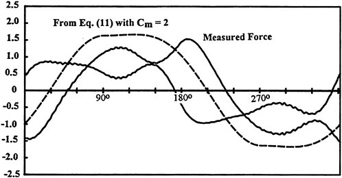
Fig. 1 Normalized measured force, force calculated from Eq. (11), and the residue (calculated—measured) force.
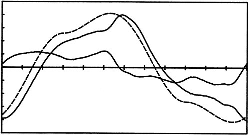
Fig. 2 Another example similar to that shown in Fig. 1. Normalized measured force, force calculated from Eq. (11), and the residue (calculated—measured) force.
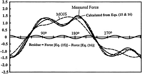
Fig. 3 Comparison of the predictions of Eqs. (15) and (16) with each other, with the measured force, and with the prediction of the MOJS equation. The residue is the difference between the predictions of Eq. (15) and (16).
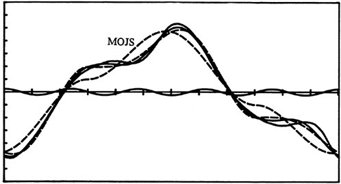
Fig. 4 Another example depicting the comparisons shown in Fig. 3.
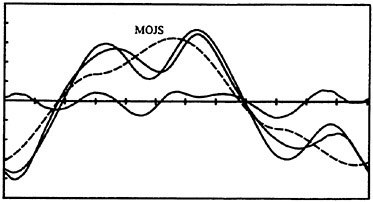
Fig. 5 Normalized force versus time for Kc=11.3, Re=53,200, and k/D=0. See Fig. 1 for scales.
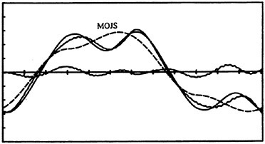
Fig. 6 Normalized force versus time for Kc=12.1, Re=54,500, and k/D=0.
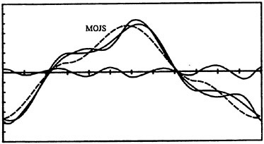
Fig. 7 Normalized force versus time for Kc=13.4, Re=37,500, k/D=0.0.
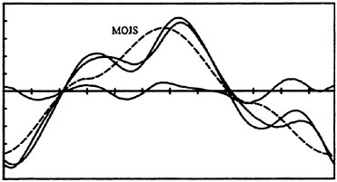
Fig. 8 Normalized force versus time for Kc=13.9, Re=31,500, k/D=0.0.
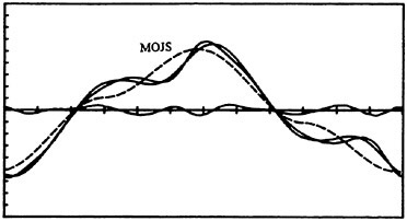
Fig. 9 Normalized force versus time for Kc=11.1, Re=72,450, k/D=1/50.
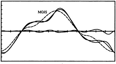
Fig. 10 Normalized force versus time for Kc=12.7, Re=62,380, k/D=1/50. See Fig. 1 for scales.
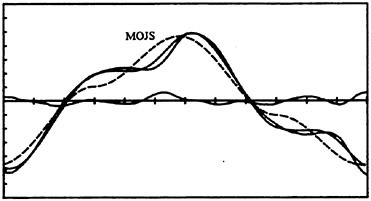
Fig. 11 Normalized force versus time for Kc=12.9, Re=84,072, k/D=1/50.
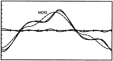
Fig. 12 Normalized force versus time for Kc=13, Re=64,072, k/D=1/50.
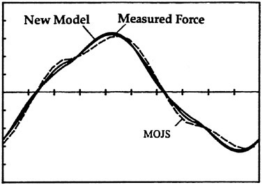
Fig. 13 Normalized force versus time for a bluff plate with Kc=2, and Re=16,000.
See Fig. 1 for scales.
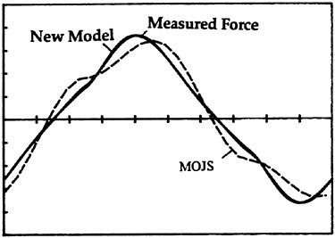
Fig. 14 Normalized force versus time for a bluff plate with Kc=5.5 and Re=16,000.
DISCUSSION
G.Hearn
University of Newcastle Upon Tyne, United Kingdom
Prof. Yeung’s question regarding the physical basis of the sin(30) term, allowed the explanation of your physics-based model to be completed during the paper presentation. Thank you both for ensuring that this happened. Fourier series arguments on their own could prevent adoption by some engineers (not all)! The explanation of how Lighthill’s modification of the MOJS equations is incomplete was nicely put. It is with sadness that we note Lighthill’s death a few weeks ago.
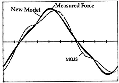
Fig. 15 Normalized force versus time for a bluff plate with Kc=6.5 and Re=192,000.
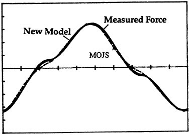
Fig. 16 Normalized force versus time for a bluff plate with Kc=24 and Re=52,000.
DISCUSSION
R.Longoria
University of Texas at Austin, USA
The plot in Figure 1 presents estimates of measured inline force induced on a fixed circular cylinder by a periodic, reversing flow. This test case, chosen from among many in this discusser’s database (1,2), demonstrates an improved predictive capability using the modified MOJS equation proposed by Prof. Sarpkaya. The drag and inertia coefficients used were found through standard Fourier-averaging, and equation 15 was applied directly. The additional term enhances the MOJS equation without introducing any auxiliary analysis or data. The reader should not judge this enhancement as obvious, especially after exploring the extensive study that has been conducted in this area by many talented researchers for four decades.
Some minor issues that Prof. Sarpkaya may have already considered are introduced here. First, should we re-examine the manner in which drag and inertia coefficients are computed from measured data? This question is prompted by an impression that Fourier-averaged coefficients may effectively filter out signal energy that is actually related to the third (harmonic) term introduced in the modified MOJS equation. Is this an invalid impression?
Second, has the effect of the nonlinearity in the drag term been overemphasized in the recent past? In light of these improved predictions, should we conclude that a more significant (and only now more tractable) uncertainty is actually due to the effect of the “concentrated vorticity” on the inertial component of inline force, especially in the drag-inertia regime?
Professor Sarpkaya foresees that we need a system perspective on problems that have and will continue to challenge naval and offshore engineering. New areas in underwater robotics, for example, will undoubtedly benefit from the insight provided in his discussion of practical modeling of fluid loads on bluff bodies. One might add that the need to further understand aperiodic flow conditions (transient, stochastic) is also set forth in the paper. If hydrodynamicists do not produce the type of reliable models promulgated by Prof. Sarpkaya, system engineers may choose to deal with fluid-structure interaction effects as mere disturbances in robust control schemes—a path that could lead to a less than optimal, and possibly catastrophic, design. There is no doubt that the modified MOJS equation presented here represents a contribution that is as significant historically as it is from a scientific and engineering standpoint.
1. Longoria, R.G., An Experimental Investigation of Hydrodynamic Forces on Circular Cylinders in Sinusoidal and Random Oscillating Flow, Ph.D. Dissertation, Mechanical Engineering Department, The University of Texas at Austin, December 1989.
2. Longoria, R.G., Beaman, J.J., and R.W. Miksad, R.W., “An Experimental Investigation of Forces Induced on Cylinders by Random Oscillatory Flow,” Journal of Offshore Mechanics and Arctic Engineering, Vol. 113, No. 4, pp. 275–285, 1991.
3 Keulegan, G.H., and Carpenter, L.H., “Forces on Cylinders and Plates in an Oscillating Fluid,” Journal of Research of the National Bureau of Standards, Vol. 60, No. 5, May 1958, pp. 423–440.
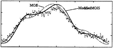
Figure 1. Normalized force versus time for Kc=15.4, Re=18,560, k/D=0.0 (data from (1)).
DISCUSSION
C.Dalton
University of Houston, USA
In this paper, Prof. Sarpkaya has provided an alternative to the traditional Morison equation, herein called the MOJS equation. Sarpkaya has modified the conventional MOJS equation by including higher harmonics without a need for determining more coefficients for their inclusion. The agreement between measured and calculated forces for the examples included in the paper is extraordinary. Equation (15), with one higher harmonic, and Equation (16), with an additional harmonic to that in Equation (15), represent the modification. As seen in the results plotted by Sarpkaya, there is very little difference between the two descriptions and, so, he recommends Equation (15) as the alternative to the conventional MOJS equation.
It is noted here that the KC values for Figures 1–4 are not included but they seem to be in the intermediate range where the drag and inertia components contribute somewhat equally. In Figures 1 and 2, the Lighthill version of the MOJS equation is plotted and, as expected, doesn’t provide good agreement with the experimentally determined force. Use of the potential flow value of the inertia coefficient, as recommended by Lighthill, doesn’t produce good agreement between measured and MOJS-predicted forces. Figures 5–12 show a comparison between the measured force and the
force predicted by both Equations (15) and (16) for intermediate values of KC and the agreement is excellent. I presume that these measured forces are all from Sarpkaya’s U-tube in which the oscillations are sinusoidal. Would there be equally good agreement when the wave motion is nonsinusoidal?
Another point to ponder is the form of the coefficient of the higher harmonic term in Equation (15). What is the basis for choosing the coefficient of the higher harmonic to be Λ|Λ|/CD? The response of Sarpkaya will be enlightening on this point.
DISCUSSION
R.Yeung
University of California at Berkeley, USA
I congratulate the author for a very worthy paper and a remarkable proposal to modify the MJOS equation. The proposed new term of sin 3\{omega}t, as a modification, is reported to be able to capture the nonlinear (higher-harmonics) behavior of the force time history associated with the “inertia term.” While this effect can be attributed to the phenomenon of vortex shedding, because of its frequency contents, it is not entirely clear what aspects of the flow would suggest a coefficient that is of the form \{Lamda}|{\Lamda}|/C_d beside the desirable feature of having the appropriate limits outside of the “inertia/drag regime.” Perhaps the author can shed more insights on this point.
There is no dispute that this provides the necessary fit of the numerous data of the author in the regime. A further point, would the proposed in-line force formula allow one to deduce a more physics-based transverse force formula? That would be of similar engineering interest.
AUTHOR’S REPLY
The comments of Professors Dalton, Longoria, Yeung, and Hearn are very much appreciated. First, the specific questions and then the broader issues (regarding the selection of Λ|Λ|/Cd) will be taken up. The measured forces are all from the author’s experiments (see Refs. [17–18] and [21–27]). The modified equation is expected to work equally-well with non-sinusoidal motions. For this purpose Eq. (15) should be re-written as
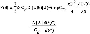
(15a)
where θ=ωt and α=3ωt. Here, U(θ) and dU(θ)/dθ represent, respectively, the velocity and acceleration for the desired non-sinusoidal motion. The meanings of Cd and Cm remain as described in the paper. I have not been able to locate data for a non-sinusoidal motion and will certainly appreciate hearing from those who have.
Prof. Longoria has provided supporting evidence (his Fig. 1). As far as Cd and Cm are concerned, nothing needs to be changed in the Fourier averaging of the force. The method of least squares yields quite similar results and is more appropriate for non-sinusoidal periodic motions. There is no question that the most important correction to the MOJS equation in the inertia/drag regime is dominated by second-order inertial forces, as exemplified by sin(3θ).
As to the coefficient of the higher harmonic, its selection is based on a number of considerations: (1) The observations of vortex shedding: In the lower half of the inertia/drag regime (7<K< 12.5), there are only two vortices at the end of a half cycle (one attached and one detached). The attached vortex soon becomes detached, while both giving rise to a new attached vortex. The two detached vortices quickly and mutually convect themselves away. The upper half of the inertia/drag regime (12.5<K<17) exhibits a similar but slightly different shedding behavior. In either case, the cycle ends with one attached and two detached vortices [5, 7]. The vortex shedding cycle shows the importance of the third harmonic and the rapid acceleration of the vortex pair shows the importance of higher order inertial forces; (2) On an extensive numerical analysis of oscillating turbulent flow about a circular cylinder (see, Sarpkaya, et al., J. OMAE, May 1977, Vol. 119, pp. 73–78); (3) On the fact that Eq. (12) immediately suggests that Λ is a fundamental inertial-force-correction parameter (see also Refs. 14 & 15); and (4) on a very
extensive analysis of the existing data [17–18, 21–27] through the use of the Fourier analysis which has ascertained that the use of Cd, Cm, C3θ, C5θ (different for each experiment) reproduces the measured force with an error (rms of the difference between the predicted force and the measured force) less than about 6 percent. This effort has also shown that no additional harmonics are needed. Then the question reduced to the discovery of a single parameter which will produce all C3θ and C5θ values in terms of K, Re, Cd, and Cm. The foregoing plus our previous efforts (Sarpkaya, [14–15]) and Eqs. (12) and (14) have suggested that a function of Λ will play a dominant role. After considerable search, a plot of all C3θ in terms of Λ|Λ|/Cd has shown that the corresponding values lie on a 45-degree line with relatively small scatter. Note that Λ/Cd is Eq. (14) and it represents the ratio of the deviation of the maximum inertial force from its ideal value to the maximum drag force (for a circular cylinder). A few more words are necessary for further clarification: (i) Many other parameters have been tried and abandoned; (ii) The Reynolds number does not directly enter into the correction of the residue, except through Cd and Cm; (iii) The term sin3θ as well as the data suggest that the most important correction to the MOJS equation in the inertia/drag regime is the higher order inertial force. This is due to the particular nature of the vortex shedding in the said regime; and (iv) The cos5θ term is a higher order drag correction and, as shown by numerous examples, is quite negligible. The simplicity of a three-term equation is certainly preferable to a slight additional correction brought about by a fourth term. Our modified MOJS equation is not analytically derivable, it does not address the transverse-force issue, and it certainly is not unique, but we would like to see better alternatives.
Obviously, much work needs to be done on transient turbulent non-periodic motions about rigid and perforated bluff bodies. Considering the current state of turbulence, I do not expect the numerical simulations to provide real-time solutions for engineering applications involving large-scale unsteadiness and non-equilibrium turbulence. If there is a heaven for the fluid dynamists of the next millennium, I am sure it will have a laboratory attached to it to build a better model.
Computation of a Wing-Body Junction Flow with a New Reynolds-Stress Turbulence Model
G.Deng, M.Visonneau (École Centrale de Nantes, France)
Abstract
The Reynolds-averaged Navier-Stokes equations are solved to calculate a wing-body junction flow. A two-equation scalar turbulence model and a new near-wall low Reynolds number second-moment closure are evaluated, holding unchanged all aspects of the numerical method. Comparisons with the experimental data collected by the Virginia Polytechnic Institute confirm the central role played by the turbulence closure in the simulation of three-dimensional vortical flows. The superior performance of the seven-equation Reynolds-stress tensor model over isotropic eddy-viscosity models is clearly established. The second-moment closure resolves accurately the development of the wing-body junction boundary layer, the formation of the spiral primary horseshoe vortex and the corner secondary vortex and the evolution of both vortices around the wing-body junction.
1 Introduction
The turbulent flow around a wing-body junction is a very complex three-dimensional flow despite a simple geometric configuration. It is encountered in many flows of engineering interest such as in aircraft wing and body junction flows, ship appendage and hull junction flows or bridge-pier flows. A wing-body junction flow is characterized by the so-called horseshoe vortex system shed around the obstacle. This vortical structure is composed by two streamwise legs of vorticity, each leg having vorticity of the opposite sense. Most often, the flow contains a region of separation around the leading edge of the obstacle, a region of strong flow acceleration between the leading edge and maximum thickness region and a region of adverse pressure gradient towards the trailing edge where flow separation may occur. For practical applications, the behaviour of this vortical structure may be of great interest since many problems like damage to support foundations, excessive level of noise or vibration have their origins in the generation of additional turbulence in the core of the horseshoe vortex. All these problems of engineering interest have motivated a great deal of experimental work studying the three-dimensional turbulent flow past a wing-body junction. Shabaka and Bradshaw [1] examined constant thickness wings with 6:1 elliptical nose, measured static pressure distribution and provided oil-film flow visualization. They carried out three-dimensional hot-wire measurements of the mean velocity and Reynolds stresses in the constant thickness region along the appendage. Their measurements revealed the strong anisotropy of the turbulence over large regions of the flow and the authors concluded that eddy-viscosity and mixing lengths models were not suitable for this type of flow.
More recently, many experimental studies were conducted at DTNSRDC (Dickinson [2]) and at the Virginia Polytechnic Institute (Devenport & Simpson [3], Fleming & al. [4], Ölçmen & Simpson [5]). All these authors examined the flow around the same geometry, e.g. a 3:2 elliptical-nosed NACA-0020-tailed cylindrical wing mounted normal to a flat plate. Dickinson [2], used X-configuration hot films, measured all Reynolds-stress components except ![]() at seven streamwise planes and provided oil-film visualization and wall-pressure measurements. Devenport & Simpson [3] developed a three-component laser anemometer to measure all the non-zero mean-velocity and Reynolds-stress components in the plane of symmetry upstream of the wing. Their measurements provided detailed informations on the structure of the attached and separated flow in the plane of symmetry and revealed bimodal histograms of veloc-
at seven streamwise planes and provided oil-film visualization and wall-pressure measurements. Devenport & Simpson [3] developed a three-component laser anemometer to measure all the non-zero mean-velocity and Reynolds-stress components in the plane of symmetry upstream of the wing. Their measurements provided detailed informations on the structure of the attached and separated flow in the plane of symmetry and revealed bimodal histograms of veloc-
ity fluctuations produced by a velocity variation that was bistable in the vicinity of the junction vortex. Fleming & al. [4] performed extensive hot-wire measurements of the mean and fluctuating velocity components at nine streamwise planes located near the wing and in the far wake in order to complement the previous database due to Dickinson [2]. Finally, Ölçmen & Simpson [5] measured the mean velocity and all Reynolds stresses from a three-velocity-component fiber-optic laser-Doppler anemometer. Their measurements were performed at seven stations along a line located in the vicinity of the primary line of separation. They established clearly the anisotropy of the turbulence and quantified the lag between the shear-stress vector direction and the flow gradient vector direction. While junction flows have generated a great deal of experimental work, numerical simulations of the flow have received relatively little attention due to the complexity of the flow field and to the occurrence of large regions of reversed flow. The first Navier-Stokes computations can be credited to Briley and McDonald [6] who used a linearized block implicit scheme with an ADI-type splitting in order to solve at low Mach numbers the compressible Navier-Stokes equations for a laminar horseshoe root vortex created by the intersection of an elliptic strut and a flat plate. Most of the other solutions were focused on high Mach number compressible flows on wing-fuselage interactions using a Baldwin-Lomax turbulence model (Gorski & al. [7]). For low speed incompressible flows, few contributions have dealt with this problem. Burke [8] have used the so-called INS3D flow solver which was based on the artificial compressibility method and used the Baldwin-Lomax model. Similar computations were carried out by Sung & Yang [9] with a four-stage explicit Runge-Kutta scheme and fourth-order explicit artificial dissipation. Chen & Patel [10] presented extensive calculations using a non-staggered grid with a finite-analytic method and a two equation k−ε turbulence model, except close to the wall where the ε was replaced by a one equation model. Deng & Piquet [11] used a fully-elliptic numerical method for solving the Reynolds-Averaged-Navier-Stokes Equations (RANSE) based on a non-staggered grid, a segregated approach and a Baldwin-Lomax turbulence model. They performed extensive comparisons of discretisation schemes (Finite-analytic, Multi-exponential, Uniexponential schemes) and concluded that the discretisation errors were not negligible on the grid used at that time (1.62 105 points). More recently, in a remarkable paper, Chen [12] pointed out the influence of modeling errors by employing a near-wall Reynolds stress closure based on a combination of the near-wall Reynolds stress model of Shima [13] and the pressure-strain correlations of Speziale & al. [14]. The calculations were carried out on a grid comprising about 3.35 105 points and the comparisons with results obtained with a two-layer isotropic eddy-viscosity model clearly revealed the superior performance of the second-moment closure. Fu & al. [15] calculated the same flow with two realizable non-linear eddy-viscosity models, retaining the wall-function approach to resolve the near-wall turbulence effect. Their computations revealed that the two nonlinear eddy-viscosity models provided overall better performance than the linear version. However, the three-dimensional boundary layer was not correctly captured, suggesting that the turbulence anisotropy was not accurately resolved by the quadratic nonlinear stress-strain relations used in their explicit turbulence closure. The lack of near-wall formulation was also a plausible explanation for the deficiencies of the proposed non-linear eddy-viscosity models.
Actually, the wing-body junction flow is an archetypal flow of great interest because of:
-
the occurrence of a large region of separated flow ahead of the wing,
-
the existence of a bi-modal regime in the vicinity of the junction vortex related to the fact that the instantaneous flow is significantly different from the mean flow,
-
the strong three-dimensionality of the flow field due to two distinct rates of strain generated independently by two different walls,
-
the strong turbulence anisotropy associated with the development of the horseshoe vortex.
All these physical characteristics associated with the availability of very detailed experimental informations on velocity components and turbulent correlations, make the VPI measurements an ideal database for evaluating the potentialities of new Reynolds-stress transport closures and, in the near future, for comparing them with Large-Eddy Simulations.
Therefore, the purpose of this article is to confront the measurements with computations based on a classical isotropic eddy-viscosity turbulence closure and a new Reynolds-stress transport closure recently developed by the authors.
2 Reynolds-stress closure
Most of three-dimensional flows contain regions of longitudinal vorticity, a physical quantity whose intensity is often underestimated by present computational codes. It is not always easy to determine the origins of such a weakness since a cautious evaluation of numerical errors versus the deficiencies of the turbulence model is still difficult to carry out for three-dimensional flows. However, the unceasing progress obtained in terms of computational power and available memory results in modeling errors being more and more predominant on numerical errors for a large category of three-dimensional industrial flows. Actually, many flows which were classified as pressure-driven flows in first approximation should be reconsidered because it is probable that the detailed dynamics of most three-dimensional flows result from a complex balance between pressure gradients and gradients of shear and normal components of the Reynolds-stress tensor. It is more and more admitted now that difficulties encountered by eddy-viscosity models in modeling complex flows are most often related to models’ inability to account for the selective amplification or attenuation of different Reynolds stresses by curvature-related strain components. These limitations are principally rooted in the fact that the eddy-viscosity models have been designed to provide the correct level of shear stress for flows in which only this stress has a predominant influence. Therefore, the essential inability of eddy-viscosity closures to simulate anisotropic turbulence can explain their bad performances on flows containing recirculating regions or intense vortices, since the turbulence anisotropy strongly influences the magnitude of longitudinal vorticity [16]. With the need to resolve anisotropy taken for granted, the main choice for new statistical turbulence closures is between nonlinear eddy-viscosity models and second-moment closures. The explicit non-linear eddy-viscosity models are very attractive because they can be seen as the most natural evolution from linear eddy-viscosity models. It is now difficult to evaluate the potentialities of such models in complex three-dimensional flows. However, some evaluations of the most recent proposals carried out by the authors suggest until now that they will perform better than linear eddy-viscosity models only on a limited range of flows characterized by a weak turbulent anisotropy. On complex three-dimensional flows, second-moment closures will have greater possibilities because of the exact representation of stress production and transport which enables realistic interactions between normal stress anisotropy and shear-stress components, even if the other physical mechanisms (diffusion, dissipation, redistribution,…) are crudely modeled, especially near the wall. Consequently, modeling of turbulence anisotropy is mandatory and then, second-moment closures are optimal candidates when high-Reynolds number flows on complex geometries are considered.
2.1 The Rij−ω model
If one wants to evaluate the true potentialities of second-moment closures on three-dimensional flows, the eviction of wall-function boundary conditions is a prerequisite, because of the frequent strong three-dimensionality of the velocity field near the wall. Therefore, a near-wall low Reynolds-number model must be constructed by introducing appropriate damping functions and additional terms. Launder & Shima [17] have proposed a very simple model that allows the Gibson & Launder model to be integrated down to the wall. Further modifications were made by Shima [18] who presented several applications for boundary-layer flows. Recent developments in near-wall second-moment closures are mainly focused on accuracy and universality by taking into account physical constraints and mathematical formalism. For example, Launder & Tselepidakis [19] attempted to improve accuracy by developing a realizable nonlinear pressure-strain model. Craft & Launder [20] tried to construct a more universal model by replacing wall normal distance and wall normal vector by Reynolds-stress invariants.
Besides accuracy and universality, efficiency is also an important issue in model development. By efficiency, it is meant here the capability for a model to provide a realistic solution with minimum computational resources. Contradictions between the model complexity induced by physical and mathematical constraints and its efficiency have already been addressed by S.Jakirlić & K.Hanjalić [21]. One of the most annoying problems for wall-flow computations with second-moment closures concerns unphysical laminarization. It is not unusual that complex model constraints are so difficult to satisfy that the algorithm can only converge towards a laminar flow which is a possible solution of the second-moment closure with given boundary conditions. Therefore, attention must be given to model development and implementation in order to avoid such unphysical laminarization. This is the reason why the authors’ objective was to build a simple and robust near-wall closure. From that point of view, it was quite natural
to try to extend the use of the turbulence frequency ω to second-moment closures.
The Rij−ω model can be considered as an extension of the Wilcox’s k−ω model to Reynolds-stress model. In a second-moment closure, the transport equation for k and ∈ can be written as:
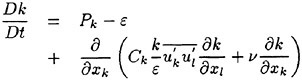
(1)
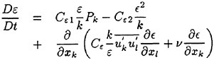
(2)
Following Wilcox, the turbulence frequency ω can be defined as:
Using this definition, a ω transport equation can be deduced from (1) and (2). When the following approximation is made:
the ω transport equation can be simplified as:
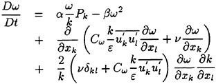
(3)
with:
Since ω is unbounded approaching the wall, the cross-diffusion term represented by the last term in the right hand side of equation (3) is numerically unstable close to the wall. In the Wilcox’s k−ω model, this term is deleted. By doing so, models based on ω formulation are completely different from those based on the ε formulation. Computationally, the ω equation is found to be far more efficient than the ε equation near the wall. However, with the help of dissipation tensor, the turbulence dissipation ε is easier to analyze, and usually, the ε equation is better calibrated than the ω equation. Consequently, to build a new near-wall closure, it is cautious to start with a well calibrated model for ε, holding unchanged all the parameters of this model away from the wall. In the present paper, a new way for constructing a near-wall model is presented, which combines the advantage of both formulations. The ε equation is first transformed into an ω equation. A damping function is introduced to cancel the cross-diffusion term in the wall region. Modifications are also made to other terms in the wall region so as to obtain a good prediction of the wall flow. This method can be applied to any existing model based on an ε equation. Based on the Shima model, a new near-wall model based on an ω equation is therefore obtained:
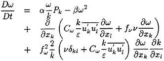
(4)
with
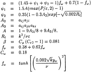
where yw is the distance to the wall.
In the present model, the function ψ1 and ψ2 proposed by Shima are kept with only a small modification on ψ1 by limiting the ratio Ρ over ε. The α coefficient as well as the kinematic viscosity ν are altered near the wall in order to obtain a good prediction for the zero pressure gradient boundary layer flow. No modification is made concerning the β coefficient that is deduced from the value Cε2=1.9. The model was calibrated by keeping unchanged the near-wall second-moment closure of Shima [18] for the modelling of diffusion, pressure-strain correlation and
dissipation terms in the six second-moment transport equations.
2.2 Model Validation
The Rij−ω model has been validated on a fully developped channel flow at Rθ=180 for which Kim, Moin & Moser’s direct simulation results [22] can be used for comparison. Results concerning this test-case were presented by Deng & Visonneau [23] who demonstrated that, although the blending function and the Cω coefficient were not calibrated for this low Reynolds number configuration, the accuracy of the original model was globally preserved. The advantages of near-wall low Reynolds-number second-moment closures have already been demonstrated by Deng & Visonneau [24] on various three-dimensional flows. A first variant of the proposed model was used to compute flows over complex geometries, namely, the flow past the HSVA Tanker (Wieghardt & Kux [25], Wieghardt [26]) and the flow through a curved rectangular duct (Kim & Patel [27]). Both computations confirmed that an accurate prediction of such vortical flows required near-wall non-isotropic turbulence models and justified resorting to a Reynolds-stress model. Finally, curvature effects observed in the duct flow were partially represented by these advanced models. The present version of the Rij−ω model has been slightly modified by calibration on the flow over a flat plate at high Reynolds numbers. The blending function fω and the coefficient Cω have been chosen such that the law of the wall was correctly reproduced for this flow. Figures 1 & 2 show the evolution of the skin-friction coefficient and the longitudinal component of the velocity with the present Rij−ω model for the turbulent flow over a flat plate ([28]).
3 Numerical method and computational details
3.1 General characteristics
All the computations presented here used a code (HORUS) entirely developped by the authors. This code is based on a partial transformation, for which the curvilinear space coordinates are used as independent, variables and the Cartesian components of velocity and pressure are retained as dependent variables. Many turbulence models are already implemented ranging from eddy-viscosity based models (one equation: Baldwin & Barth’s model [29]; two equations:
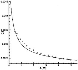
Figure 1: Skin-friction coefficient distribution. Solid line: Rij−ω model; symbols: experiment (from [28]).
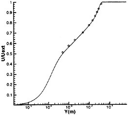
Figure 2: Mean velocity profile at X=3.187 m and Reθ=10861; solid line: Rij−ω model; symbols: experiment (from [28]).
k−ε models (Chen & Patel [30], Nagano & Tagawa [31], Deng & Piquet [32]), k−ω models (Wilcox, Menter BSL and SST modified versions [33], [34])) to models requiring the solution of Reynolds Stress Transport Equations (Shima’s model [18], and variants developed by the present authors). To avoid any wall-function boundary conditions which turn out to be unacceptable when three-dimensional flows are considered, near-wall low-Reynolds number treatments are systematically implemented in the aforementioned turbulence models.
A structured cell-centered layout is used in which the pressure, turbulence and velocity unknowns share the same location. The momentum and continuity equations are coupled through the PISO procedure with the help of the Rhie & Chow flux interpolation procedure and several implicit second order accurate
schemes are implemented for the space and time discretisations.
Preconditioned conjugate gradient solvers (CGS, CGSTAB) are used to solve the linear systems.
This code can be used with most of the current mathematical boundary conditions and additional no-slip condition can be added inside the computational domain to enable the computation of configurations of intermediate complexity (after-body+ nozzle, for instance) without having recourse to a multi-block approach. A multi-block extension, currently based on point-to-point coincident blocks, has been developed and is currently used on complex geometries. The more promising “Chimera” approach, based on overlapping grids, is now under development to make it possible the computations of flows around industrial configurations.
3.2 A peculiar numerical treatment
Second-moment closures are particularly difficult to include into a time-implicit RANSE solver because of:
-
the absence of the numerically stabilizing eddy viscosity,
-
the strong coupling between anyone stress and strains other than the ones linked to that stress via the Boussinesq relations,
-
the predominant influence in the momentum transport equations of equilibrium between several source terms, namely, the pressure and Reynolds-stress gradients,
-
the complexity of second-moment transport equations through added non linearities introduced by the actual low-Reynolds near-wall formulations.
Moreover, the incorporation of second-moment closures into solvers designed for flows around complex geometries is considerably complicated by the mandatory use of colocated variable arrangement. Different numerical strategies have been designed to enhance stability in this context. Some authors [35], enforce stability by extracting apparent turbulent viscosity from the source terms of second-moment transport equations. On the other hand, [36] developed a fully coupled implicit resolution of momentum and second-moment transport equations to avoid velocity-turbulence decoupling. More recently, several authors [37], [38], have employed explicit time-marching procedures, often based on a four-stage Runge-Kutta scheme for the mean flow equations, without reporting any severe stability problem. In [39], Deng & Visonneau suggested that a likely cause of unstability was the discrete disequilibrium between pressure and Reynolds-stress gradients which are treated as explicit source terms in the momentum equations. When one source term is clearly dominant over the other one, the solution is monotonous but as soon as both source terms are almost equal and of opposite signs, the magnitude of the velocity will be small and non monotonous. Erratic oscillations of a component of the velocity even very small in absolute value, lead almost invariably to the divergence of the algorithm. They proposed several drastic modifications of the velocity-pressure coupling algorithm to achieve a perfect balance between pressure and turbulent stresses gradients. The reader is referred to [39] where the modifications of the original PISO algorithm are explained in detail.
4 Results and discussion
4.1 Grid topology and boundary conditions
The calculations were performed at the experimental Reynolds number of 5.0 105 on a grid comprising 90× 82×82 nodes, in the streamwise, normal to the wing, and vertical directions. The first coordinate surfaces off the solid walls were located at y+≈1.0 (where y+=uτyn/ν, uτ is the wall friction velocity and yn is the normal distance to the wall) with about 15 points within the sublayer and the buffer layer. The solution domain is defined by −2.0<Χ/C<28., 0.<Y/C<2.0 and 0.<Ζ/C<0.8 where C is the chord length of the wing and the external boundary conditions are provided by previous infinite flat plate computations. A typical view of the grid is given in Fig. 3. Symmetry conditions are specified at the two planes of symmetry ξ=1 and η=1 (excepts on the wing). At the external boundary, η=ηΜΑΧ, velocity profiles and Reynolds stress components are specified by a previous infinite flat plate computation. On all the walls (ζ=1 and η=1), no-slip conditions are specified. The wing is considered to be infinite and therefore ζ=ζMAX is an horizontal plane of symmetry.
4.2 Topology of the flow
To explore the structure of the horseshoe vortex predicted by both turbulence models, plots of particle
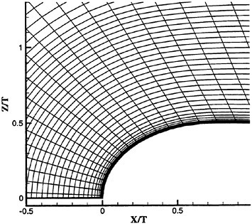
Figure 3: Detailed view of the grid near the nose of the wing
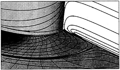
Figure 4: k−ε model- Particle traces in the symmetry plane and on the flat plate (the pressure contours are visible on the flat plate)
traces in the plane of symmetry and on the flat plate are shown in Figs. 4 and 5. The Rij−ω solution is characterised by a spiral vortex which is not present in the k−ε solution. Both models predict a primary line of separation located at the intersection between the three-dimensional surface and the flat plate. However, the low-shear stress line which was observed in the experiments between the wing and the primary line of separation is only visible in the second-moment solution, indicating that the secondary motion predicted by the anisotropic turbulence closure is far more intense.
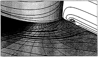
Figure 5: Rij−ω model- Particle traces in the symmetry plane and on the flat plate (the pressure contours are visible on the flat plate)
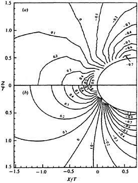
Figure 6: Measured pressure coefficient on the flat plate, (a) measurements, (b) calculated for freestream, (from [3])
4.3 Pressure distribution and wall-flow on the flat plate
Figure 6 shows contours of mean static pressure coefficient Cp measured on the flat plate in the vicinity of the nose of the wing. An interesting feature is the distortion of the measured contours that occurs close to the wing. This distortion is due to the lowering of the pressure in the junction vortex. Figure 7 shows the static pressure coefficient Cp calculated with the two different turbulence closures, namely, the Chen & Patel k−ε model and the newly proposed Rij−ω closure. Whereas the computations based
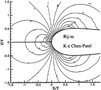
Figure 7: Pressure coefficient on the flat plate, (a) Rij−ω model, (b) Chen & Patel k−ε model
on the isotropic closure do not reveal any distortion of the pressure coefficient, the pressure contours obtained with the Rij−ω closure are significantly distorted close to the wing. This pressure bulge is clearly related to the far more intense vortical motion predicted by the second-moment closure in the core of the horseshoe structure.
Figure 8 displays a surface oil-flow visualization performed in the vicinity of the nose of the wing. A line of separation emanates from a saddle point located at 0.47T (T is the maximum thickness of the wing) upstream of the wing leading edge. This line is less intense than a second line emanating closer to the nose of the wing from a point located at 0.28T upstream of the wing. According to Devenport & Simpson [3], this line is not a separation line but a line of low streamwise shear which divides the separated flow into two zones: a region of high streamwise shear stresses near the wing and a strip of lower shear stresses upstream.
Figure 9 shows the velocity vectors and the limiting streamlines on the wall around the wing nose provided by the two turbulence models on the same grid. The convergence of the first line of separation is more pronounced with the Rij−ω model than with the k−ε model. The most interesting feature is the dramatic difference between the two turbulence closures concerning the inner line of low streamwise shear stress. Whereas the k−ε solution does not reveal any second line of convergence, the anisotropic Rij−ω solution
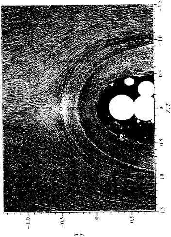
Figure 8: Surface oil-flow visualization on the flat plate (from [3])
clearly captures the correct topology of the wall flow. The line of low streamwise shear stress is well marked, located at 0.21T upstream of the wing, wraps around the leading edge and merges with the primary line of separation alongside the wing. The strong variation of the shear is clearly illustrated by the velocity field close to that line.
For the sake of brevity, no comparisons on the velocity profiles and turbulent stresses in the vertical plane of symmetry are provided in the present paper. However, it is important to mention that the comparisons revealed large discrepancies between both numerical results and the experiments near the nose of the wing (−0.30<X/T<−0.1536). The intensity of normal turbulent stresses ![]() and
and ![]() was severely underestimated by both turbulence closures. This deficiency must be correlated with the bi-modal structure of the flow in this region.
was severely underestimated by both turbulence closures. This deficiency must be correlated with the bi-modal structure of the flow in this region.
4.4 Results on X=cst. planes
Extensive mean and fluctuating velocity measurements were also conducted by Fleming & al. [4]
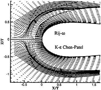
Figure 9: Wall-limiting velocity vectors on the flat plate, (a) Rij−ω model, (b) Chen & Patel k−ε model
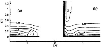
Figure 10: Contours of U/Uref at X/C=0.64, (a) Experiments; (b) k−ε model
at several Χ/C=cst. planes adjacent to the wing and in the wake. These measurements made it possible to characterise the horseshoe vortex development. For the sake of brevity, only two stations, namely Χ/C=0.64; 1.50 are chosen to compare the respective performances of k−ε and Rij−ω models. Figures 10 and 11 show the near-wing contours of U/Uref with both turbulence models at Χ/C=0.64.
The distortion of the iso-velocity contours observed in the measurements are due to the secondary motion which transports higher momentum fluid from the edge of the boundary layer to the near-wall region. This trend is severely underestimated by the k−ε solution and accurately reproduced by the anisotropic Rij−ω model which yields a more intense vortical crossflow. Figures 12 and 13 show the contours of the rms Reynolds normal stress u′/Uref at the same sta
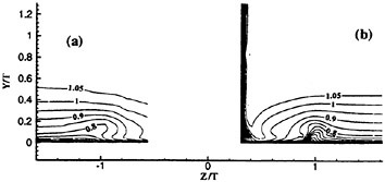
Figure 11: Contours of U/Uref at Χ/C=0.64, (a) Experiments; (b) Rij−ω model
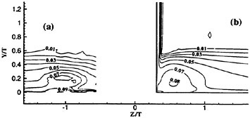
Figure 12: Contours of u′/Uref at Χ/C=0.64, (a) Experiments; (b) k−ε model
tion. A local maximum is located in the region where the distorsion of U/Uref contours occurs, indicating that this local peak of turbulence is probably due to the increased mixing of the boundary layer fluid by the horseshoe vortex. The k−ε solution exhibits a large zone of high normal stress located in the corner between the wing and the flat plate. This high turbulence intensity generates an excessive level of turbulent viscosity which absorbs the secondary motion in the core of the horseshoe vortex. On the contrary, the anisotropic second-moment closures provides a much more physical solution since the local peak of u’ is accurately positionned, even if its maximum level is Somewhat underestimated.
Figures 14 and 15 show the isowakes in the near wake at Χ/C=1.50 and figures 16 to 17 display the corresponding Reynolds normal stress u’. Here, under the joint action of near-wall pressure-induced crossflow and vortex-induced secondary flow, the distortions of iso-velocity contours are less pronounced, indicating that the longitudinal vorticity is somewhat relaxed. This tendency is accurately reproduced by the k−ε solution. However, this limited success is rather due to the fact that the longitudinal vorticity field predicted by this closure at the upstream stations was severely underestimated. Contrary to
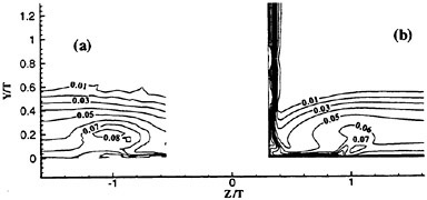
Figure 13: Contours of u′/Uref at Χ/C=0.64, (a) Experiments; (b) Rij−ω model
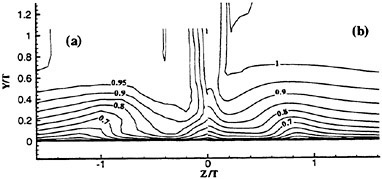
Figure 14: Contours of U/Uref at Χ/C=1.50, (a) Experiments; (b) k−ε model
the isotropic model, the second-moment solution indicates a slower than measured decay of the secondary motion.
This trend was already noticed by Sotiropoulos & Patel [40] who used the original Shima model to compute the growth and decay of longitudinal vortices in a straight circular-to-rectangular transition duct. Therefore, it is plausible that this inability to capture the recovery of the flow in the wake should be attributed to the modeling of the Reynolds-stress trans
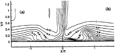
Figure 15: Contours of U/Uref at Χ/C=1.50, (a) Experiments; (b) Rij−ω model
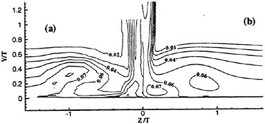
Figure 16: Contours of u′/Uref at Χ/C=1.50, (a) Experiments; (b) k−ε model
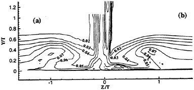
Figure 17: Contours of u′/Uref at Χ/C=1.50, (a) Experiments; (b) Rij−ω model
port equations.
4.5 Velocity profiles and turbulent stress profiles along a specific line
In a more recent study, Ölçmen & Simpson [5] have measured the velocity profiles and all Reynolds stresses at seven stations located along a line determined by the mean velocity vector component parallel to the wall in the layer where ![]() is maximum. The locations of measurements are described in figure 18. All the velocity and Reynolds stress components are given in their respective local free-stream coordinate axes. In the computations, the free-stream coordinates are provided by the velocity directions at the first point (from the wall) where U=0.995Uext. For the sake of brevity, only three stations, namely, stations 3, 5 and 7, are selected for discussion in this paper. All the results are plotted with semi-logarithmic coordinates.
is maximum. The locations of measurements are described in figure 18. All the velocity and Reynolds stress components are given in their respective local free-stream coordinate axes. In the computations, the free-stream coordinates are provided by the velocity directions at the first point (from the wall) where U=0.995Uext. For the sake of brevity, only three stations, namely, stations 3, 5 and 7, are selected for discussion in this paper. All the results are plotted with semi-logarithmic coordinates.
4.5.1 Mean velocity profiles
Figs. 19, 20 & 21 display the mean velocity profiles at stations 3, 5 & 7. All the figures show that both tur-
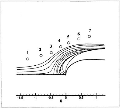
Figure 18: Locations of the velocity and stress measurements
bulence models simulate reasonably well the general trends of the mean flow field.
However, the Rij−ω closure provides systematically a better representation of the three-dimensionality of the flow. The longitudinal U-component is always in better accordance with the experiments and the W-component is more intense than the one calculated with the k−ε model. For
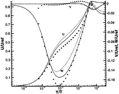
Figure 19: Velocity profiles in free-stream coordinates at station 3. Solid line: Reynolds-stress model; dashed line: k−ε model; symbols: experiment
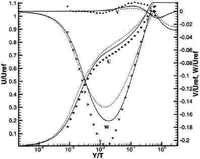
Figure 20: Velocity profiles in free-stream coordinates at station 5. Solid line: Reynolds-stress model; dashed line: k−ε model; symbols: experiment
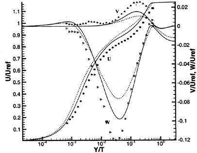
Figure 21: Velocity profiles in free-stream coordinates at station 7. Solid line: Reynolds-stress model; dashed line: k−ε model; symbols: experiment
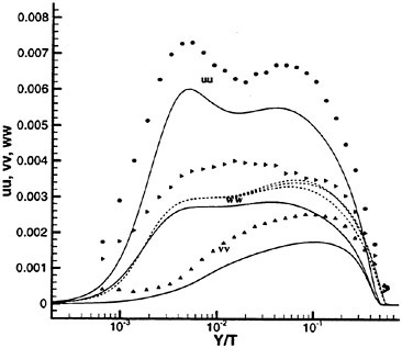
Figure 22: Normal stress components in free-stream coordinates at station 3. Solid line: Reynolds-stress model; dashed line: k−ε model; symbols: experiment
instance, at station 5 (Fig. 20), the k−ε model predicts for the W-component of the velocity a minimum value of −0.15, whereas the Rij−ω closure provides a value of −0.18, the experimental value being around −0.21. Therefore, even if the Rij−ω model still overestimates the U-component and under-estimates the W-component, it is clear that the even imperfect simulation of turbulence anisotropy has dramatically increased the three-dimensionality of the flow towards the solution revealed by the measurements.
4.5.2 Normal turbulent stresses
Figs. 22, 23 & 24 show the normal turbulent stresses at the same stations 3, 5 & 7. As expected, the k−ε closure is not able to discriminate between the three normal stresses which are roughly identical to 2k/3. The normal stresses computed with the new Rij−ω closure agree reasonably well with the experimental results. From stations 3 to 7, ![]() increases continuously in the vicinity of the wall and decreases in the outer region. This trend is closely simulated by the Rij−ω closure although the magnitude of that stress is slightly underestimated.
increases continuously in the vicinity of the wall and decreases in the outer region. This trend is closely simulated by the Rij−ω closure although the magnitude of that stress is slightly underestimated.
The ![]() correlation increases more gradually and reaches a plateau from y/T comprised between 10−2 and 510−1. This particular behaviour is well simulated by the anisotropic closure which, hereagain, underestimates the magnitude of this normal stress.
correlation increases more gradually and reaches a plateau from y/T comprised between 10−2 and 510−1. This particular behaviour is well simulated by the anisotropic closure which, hereagain, underestimates the magnitude of this normal stress.
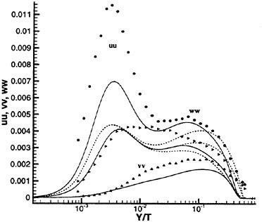
Figure 23: Normal stress components in free-stream coordinates at station 5. Solid line: Reynolds-stress model; dashed line: k−ε model; symbols: experiment
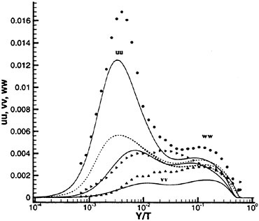
Figure 24: Normal stress components in free-stream coordinates at station 7. Solid line: Reynolds-stress model; dashed line: k−ε model; symbols: experiment
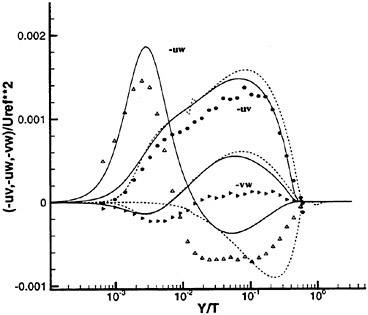
Figure 25: Shear stress components in free-stream coordinates at station 3. Solid line: Reynolds-stress model; dashed line: k−ε model; symbols: experiment
The ![]() correlation increases more rapidly near the wall and reaches a plateau closer to the wall than
correlation increases more rapidly near the wall and reaches a plateau closer to the wall than ![]() . This behaviour is well captured by the anisotropic model even if the computed normal stress is slightly underevaluated in the outer region of the boundary layer.
. This behaviour is well captured by the anisotropic model even if the computed normal stress is slightly underevaluated in the outer region of the boundary layer.
4.5.3 Turbulent shear stresses
Figs. 25, 26 & 27 show the turbulent shear stresses at the same stations as before. As expected, both models provide similar simulations of ![]() and
and ![]() shear stresses.
shear stresses.
The slight irregularities which can be observed on the k−ε results are due to the lack of continuity of derivatives through the boundaries between the two layers defined in Chen & Patel model. ![]() is accurately predicted by both models but
is accurately predicted by both models but ![]() is severely overerestimated in the outer region of the boundary layer. The most remarkable feature in these comparisons is the dramatic difference concerning the computations of
is severely overerestimated in the outer region of the boundary layer. The most remarkable feature in these comparisons is the dramatic difference concerning the computations of ![]() has a local maximum value close to the wall and starts developping to reach an adimensional maximum value of 0.003 at station 5 with a change of sign occurring at Y/T≈210−2 for most of the stations. This behaviour is absolutely ignored by the computations based on the k−ε closure which even do not predict the negative value of
has a local maximum value close to the wall and starts developping to reach an adimensional maximum value of 0.003 at station 5 with a change of sign occurring at Y/T≈210−2 for most of the stations. This behaviour is absolutely ignored by the computations based on the k−ε closure which even do not predict the negative value of ![]() in the outer region at station 7 (Fig. 27).
in the outer region at station 7 (Fig. 27).
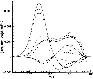
Figure 26: Shear stress components in free-stream coordinates at station 5. Solid line: Reynolds-stress model; dashed line: k−ε model; symbols: experiment
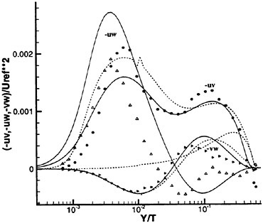
Figure 27: Shear stress components in free-stream coordinates at station 7. Solid line: Reynolds-stress model; dashed line: k−ε model; symbols: experiment
On the other hand, the computations based on the anisotropic Rij−ω closure represent fairly well this evolution, even if the maximum value of this turbulent shear stress is hereagain slightly overestimated. The simulation of turbulence anisotropy creates the mechanism for predicting the correct near-wall behaviour of the turbulent shear stress that is the most correlated to the three-dimensionality of the flow. The complex coupling between the normal and shear turbulent stresses is correctly accounted for by the present Rij−ω closure which provides a dramatically new physical solution much closer to the measurements than the solution obtained with k−ε model.
5 Summary and conclusion
The two-equation, two-layer, k−ε model of Chen & Patel and a new seven-equation Reynolds-stress transport model based on the model of Shima [18] in which a new transport equation for the turbulent frequency ω was implemented, were employed to calculate the flow around a wing-body junction. For both models, the flow was resolved up to the wall and all numerical characteristics (spatial discretization, numerical schemes, initial and boundary conditions) were held invariant to evaluate the importance of turbulence model in the computation of a wing-body junction flow. Each computations were compared with the extensive experimental database generated by the Virginia Polytechnic Institute during more than eight years. This systematic evaluation lead to the following conclusions:
-
All the comparisons with global and local quanti-| ties, ranging from the velocity components to the Reynolds-stress tensor components have established the clear superiority of the second-moment closure. This new Reynolds-stress transport model accurately reproduced the anisotropic behaviour of the normal Reynolds stress components, which led to a clear amplification of the longitudinal vorticity. Moreover, the Reynolds stress anisotropy was also responsible for the strong augmentation of the shear stress
 close to the horizontal plane. This result clearly demonstrated that second-moment calculations were particularly well suited to three-dimensional vortical flows involving several predominant flow gradients.
 -
As expected, near the leading edge of the wing, the statistical second-moment model provided a solution which was significantly different from what was observed by [3]. The simulation of the flow in that region is somewhat out of the scope of a steady second-moment turbulent simulation since the flow appears to be characterised by a large scale unsteadiness. It would be of great interest to use this database to assess the actual potentialities of Coherent-Structure-Capturing methods [41] to determine the respective domain of applications and computational resources required by statistical second-moment closures and Large-Eddy-Simulations methods.
6 Acknowledgments
Tabulated experimental data and flow visualization photographs were kindly provided by Prof. R.L. Simpson. Thanks are due to the Scientific Committee of IDRIS and the DS/SPI for attributions of Cpu on the VPP and T3E on which most of the calculations were performed.
References
[1] I.M.M.A Shabaka and P.Bradshaw, “Turbulent flow measurements in an idealized wing/body junction,” ΑΙΑA J., Vol. 19, No. 2, 1981, pp. 131–132.
[2] S.C.Dickinson, “An experimental investigation of appendage-flat plate junction flow,” DTNSRDC Report 86/052, Vol. 1–2, 1986.
[3] W.J.Devenport and R.L.Simpson, “Time-dependent and time-averaged turbulence structure near the nose of a wing-body junction,” Journal of Fluid Mechanics, Vol. 210, 1990, pp. 23–55.
[4] R.L.Simpson J.L.Fleming and W.J.Devenport, “An experimental study of a turbulent wing-body junction and wake flow,” Experiments in Fluids, Vol. 14, 1993, pp. 366–378.
[5] S.M.Ölçmen and R.L.Simpson, “An experimental study of a three-dimensional pressure-driven turbulent boundary layer,” Journal of Fluid Mechanics, Vol. 290, 1995, pp. 225–262.
[6] W.R.Briley and H.McDonald, “Computations of three-dimensional horseshoe vortex flow using the Navier-Stokes equations,” Proceedings of the 7th ICNMFD Conf. Stanford, 1980.
[7] T.R.Govindan J.J.Gorski and B.Lakshminarayana, “Comparison of three-dimensional turbulent shear flow in corners,” ΑΙΑA J., Vol. 23, No. 12, 1985, pp. 685–692.
[8] R.W.Burke, “Computation of turbulent incompressible wing-body junction flow.” AIAA Paper 89–0279, 1989.
[9] C.H.Sung and C.I.Yang, “Validation of turbulent horseshoe vortex flows,” Proceedings of the 17th ONR Symposium on Naval Hydrodynamics, The Hague, The Netherlands, 1988, pp. 241–255.
[10] H.C.Chen and V.C.Patel, “The flow around wing-body junctions,” Proceedings of the 4th Symposium on Numerical and Physical Aspects of Aerodynamic Flows, Long Beach, CA, 1989, pp. 16–19.
[11] G.B.Deng and J.Piquet, “Computation of the flow past an airfoil-flat plate junction,” Int. J. Num. Meth. Fluids, Vol. 15, 1992, pp. 99–124.
[12] H.C.Chen, “Assessment of a Reynolds stress closure model for appendage-hull junction flows,” Journal of Fluids Engineering, Vol. 117, 1995, pp. 557–563.
[13] N.Shima, “A Reynolds-stress model for near-wall and low-Reynolds-number regions,” Journal of Fluids Engineering, Vol. 110, 1988, pp. 38–44.
[14] C.G.Speziale, S.Sarkar, and T.B.Gatski, “Modeling the pressure-strain correlation of turbulence: An invariant dynamical systems approach,” Journal of Fluid Mechanics, Vol. 227, 1991, pp. 245–272.
[15] T.Rung S.Fu, Z.Zhai and F.Thiele, “Numerical study of flow past a wing-body junction with a realizable nonlinear EVM,” Proceedings of the 11th Turbulent Shear Flows, 1997, pp. 6–7–6–12.
[16] C.G.Speziale, “On turbulent secondary flows in pipes of non circular sections,” Int. J. Eng. Sci., Vol. 20, 1982, pp. 863–872.
[17] B.E.Launder and N.Shima, “Second-Moment Closure for the Near-Wall Sublayer: Development and Application,” AIAA Journal, Vol. 27, 1989, pp. 1319–1325.
[18] N.Shima, “Prediction of turbulent boundary layers with a second moment closure,” Journal of Fluids Engineering, Vol. 115, 1993, pp. 1–27.
[19] B.E.Launder and D.P.Tselepidakis, “Progress and Paradoxes in Modelling Near-Wall Turbulence,” Proceedings of the 8th Symposium on Turbulent Shear Flows, Munich, 1991, pp. 29–1–29–6.
[20] T.J.Craft and B.E.Launder, “Improvments in near-wall Reynolds stress modelling for complex flow geometries,” Proceedings of the 10th Turbulent Shear Flows, 1995, pp. 20–25–20–30.
[21] S.Jakirlić and K.Hanjalić, “A Second-Moment Closure for Non-Equilibrium and Separating High- and Low-Re-Number Flow,” Proceedings of the 10th Symposium on Turbulent Shear Flows, Pennsylvania, 1995, pp. 23–25–23–30.
[22] J.Kim, P.Moin, and R.Moser, “Turbulence Statistics in Fully Developed Channel Flow at Low Reynolds Number,” J. Fluid Mech., Vol. 177, 1987, pp. 133–166.
[23] G.B.Deng and M.Visonneau, “Near-wall modelization for dissipation in second-moment closures,” Proceedings of the 11th Turbulent Shear Flows, 1997, pp. P2–101–P2–106.
[24] G.B.Deng and M.Visonneau, “Assessment of second-moment turbulence closures for three-dimensional vortical flows,” Proceedings of the 1997 ASME Fluids Engineering Division Summer Meeting, 1997.
[25] K.Wieghardt and J.Kux, “Nomineller nachstrom auf grund von windkanal versuchen,” Jahrb. der Schiffbau Technischen Gesellschaft (STG), 1980.
[26] K.Wieghardt, “Kinematics of ship wake flow,” Proceedings of the 7th David Taylor Memorial Lecture, DTNSRDC Report 81/093, 1982.
[27] W.J.Kim and V.C.Patel, “Origin and decay of longitudinal vortices in developing flow in a curved rectangular duct,” Journal of Fluids Engineering, Vol. 116, 1994, pp. 45–52.
[28] Computation of Turbulent Boundary Layers—1968 AFOSR-IFP-Stanford Conference, D.E. Coles & E.A.Hirt, ed., 1968.
[29] B.S.Baldwin and T.J.Barth, “A one equation turbulence transport model for high Reynolds number wall-bounded flows,” AIAA 29th Aerospace Sciences Meeting, AIAA Paper 91–0610, 1991.
[30] H.C.Chen and V.C.Patel, “Practical near-wall turbulence models for complex flows including separation.” AIAA-87–1300, 1987.
[31] Y.Nagano and M.Tagawa, “An improved k−ε model for boundary layers flows,” Journal of Fluids Engineering, Vol. 100, 1990, pp. 33–39.
[32] G.B.Deng and J.Piquet, “k−ε turbulence model for low-Reynolds number wall-bounded shear flow,” Proceedings of the 8th Turbulent Shear Flows, 1991, pp. 26–2–26–7.
[33] D.C.Wilcox, “Reassessment of the scale-determining equation for advanced turbulence models,” AIAA Journal, Vol. 26, 1988, pp. 1299–1310.
[34] F.R.Menter, “Zonal two-equations k−ω turbulence models for aerodynamic flows,” AIAA 24th Fluid Dynamics Conf., AIAA Paper 93–2906, 1993.
[35] F.S.Lien and M.A.Leschziner, “Computational modelling of multiple vortical separation from streamlined body at high incidence,” Proceedings of the 10th Turbulent Shear Flows, 1995, pp. 4–19–4–24.
[36] S.Sebag, V.Maupu, and D.Laurence, “Nonorthogonal calculation procedures using second moment closure,” Proceedings of the 8th Turbulent Shear Flows, 1991, pp. 20–3–20–8.
[37] F.Sotiropoulos and V.C.Patel, “Second moment modelling for ship-stern and wake flows,” Proceedings of the CFD Workshop for Improvment of Hull Form Designs—Tokyo, Ship Research Institute, ed., 1994, pp. 187–198.
[38] L.Davidson, “Reynolds stress transport modelling of shock-induced separated flow,” Computers & Fluids, Vol. 24–3, 1995, pp. 253–268.
[39] G.B.Deng and M.Visonneau, “Evaluation of eddy-viscosity and second-moment turbulence closures for steady flows around ships,” Proceedings of the 21st Symposium on Naval Hydrodynamics, 1996, pp. 453–469.
[40] F.Sotiropoulos and V.C.Patel, “Prediction of turbulent flow through a transition duct using a second-moment closure,” ΑΙΑA Journal, Vol. 32–11, 1994, pp. 2194–2204.
[41] J.H.Ferziger, “Large eddy simulation,” Simulation and Modeling of Turbulent flows, M.Y.Hussaini and T.Gatski, eds., Cambridge University Press, 1995.
DISCUSSION
C.H.Sung and M.J.Griffin
Naval Surface Warfare Center, Carderock Division, USA
There is no doubt that of all the turbulence models, the Reynolds Stress model contains the most physics and should be pursued.
To avoid hot-wiring in a production code, it is important that normal wall distances do not appear in the model. We would like to hear authors’ comments on the robustness of the damping functions used. In particular, if they work in flat-plate, do they also work in body at incidence without changing their values? The damping function fw which contains normal wall distance is of particular interest. What is the prospect of eliminating the normal wall distance from this function?
We pursue nonlinear two-equation models. The vortex in front of the wing computed using Speziale’s quadratic non-linear k-w model is shown below:
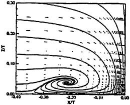
It can be seen that the predicted vortex formation compares favorably with the experiment when three different turbulence models are used, as presented by A. Rizzi & J.Vos (AIAA Journal, Vol. 36, May 1998) and shown below:
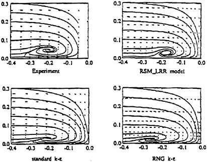
AUTHORS’ REPLY
Wall damping function is usually constructed by using one of the three parameters: y+=yuτ/ν, ![]() and Rτ=k2/(νε). In the authors’ opinion, it is not desirable to use a wall related parameter which changes during temporal or nonlinear iteration, such as uτ. Compared with Rτ, Ry is a more representative wall-distance indicator. Models based on Ry are usually more stable that those based on Rτ. Although the wall normal distance is difficult to determine exactly for complex geometries, a numerical approximation is easy to implement. The authors use a body-fitted multi-block solver that is capable of computing the wall normal distance for any given grids. More complex geometries such as the HSVA tanker have been treated without changing anything with the same code. The authors do not feel the need to replace Ry in the wall damping function for the application in complex geometries. However, when using a moving grid, the computation of wall-normal distance may become very time consuming. In this case, models based on Rτ will become attractive.
and Rτ=k2/(νε). In the authors’ opinion, it is not desirable to use a wall related parameter which changes during temporal or nonlinear iteration, such as uτ. Compared with Rτ, Ry is a more representative wall-distance indicator. Models based on Ry are usually more stable that those based on Rτ. Although the wall normal distance is difficult to determine exactly for complex geometries, a numerical approximation is easy to implement. The authors use a body-fitted multi-block solver that is capable of computing the wall normal distance for any given grids. More complex geometries such as the HSVA tanker have been treated without changing anything with the same code. The authors do not feel the need to replace Ry in the wall damping function for the application in complex geometries. However, when using a moving grid, the computation of wall-normal distance may become very time consuming. In this case, models based on Rτ will become attractive.
One of the most important contributions of the Reynolds stress transport model to the prediction of the wing-body junction flow is a better description of normal stress anisotropy and the exact description of the convection effect of Reynolds stress which is found to be very important in front of the wing. Results shown by the discussers are very interesting. It indicates that by taking into account the normal stress anisotropy with a nonlinear two-equation model, one can improve prediction of the horse-shoe vortex. However, the nonlinear two-equation models which are deduced from a Reynolds stress transport model by using local equilibrium assumption, are obviously unable to account for the convection effect. Consequently, other important features such as the distinction of high shear stress and low shear stress regions, the position of the pigment accumulation line, etc., captured by the Reynolds stress transport model, are unable to be predicted with nonlinear models.
Predictions with a Reynolds stress transport model given by A.Rizzi are not representative. They are probably obtained with a wall function approach, which suggests that wall function approach should not be used for complex three-dimensional flow prediction. In the present studies, the authors use a low Reynolds number model where wall reflection terms need to be added. Unfortunately, just like the wall function approach, the wall reflection terms are calibrated with simple boundary layer flow. The present study shows that they are not valid for separated flows. The shape of the horse-shoe vortex predicted by the Reynolds stress transport model is presented in the following figure. It is less satisfactory than the result obtained by the discussers with a nonlinear two-equation model, which indicates that the improvement provided by an exact description of convection effect is smaller than the deterioration introduced by the wall reflection terms.
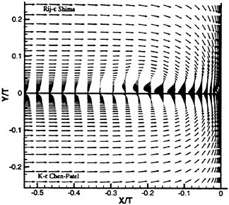
Velocity vectors in the vertical symmetry plane.


