
Incipient Breaking of Steady Waves
M.Miller, T.Nennstiel, L.Fialkowski, S.Pröstler, J.Duncan, A.Dimas
(University of Maryland, USA)
Abstract
The effect of free-surface drift layers on the maximum height that a steady wave can attain without breaking is explored through experiments and numerical simulations. In the experiments, the waves are generated by towing a two-dimensional fully submerged hydrofoil at constant depth, speed, and angle of attack. The drift layer is generated by towing a plastic sheet on the water surface ahead of the hydrofoil. It is found that the presence of this drift layer (free surface wake) dramatically reduces the maximum nonbreaking wave height and that this wave height correlates well with the surface drift velocity. Direct numerical simulations of the two-dimensional Euler equations are used for non-breaking and incipient breaking conditions. Initially symmetric wave profiles are superimposed on a parallel drift layer whose mean flow characteristics match those in the experiments. It is found that for large enough initial wave amplitudes a bulge forms at the crest on the forward face of the wave and the small scale vorticity fluctuations just under the surface in this region grow dramatically in time. This behavior is taken as a criterion to indicate impending wave breaking. The maximum nonbreaking wave elevations obtained in this way are in good agreement with the experimental findings. For breaking conditions, large wave simulations of the corresponding filtered Euler equations are performed. The results exhibit a vortex formation on the forward the face of the breaker. This feature of the flow is qualitatively similar to experimental observations.
1 Introduction
The steady free surface flow field generated by a ship moving at constant speed in calm water typically includes breaking waves at the bow and the stern. The bow wave and the parts of the stern wave far from the ship’s track propagate in undisturbed water; however, the parts of the stern wave near the ship track propagate in a flow with a free surface shear layer due to the boundary layer of the hull and/or the surface wakes of upstream breaking waves. (Surface wakes of steady breaking waves have been studied by Battjes and Sakai [1] and Duncan [2] and [3].) A comprehensive theoretical or numerical model of wave breaking in the presence of surface wakes must include information on incipient wave breaking conditions. An incipient breaking wave is defined as a nonbreaking wave for which even a slight increase in its steepness would cause breaking. The fact that upstream surface wakes affect the incipient breaking conditions of downstream waves is demonstrated by observations that the breaking stern wave crest frequently extends out past the side of the ship to a width equal to the width of the breaking bow wave, even when the stern wave steepness appears to be very low in terms of calm water incipient breaking conditions. These effects are illustrated in the photograph shown in Parker [4].
The incipient breaking condition for steady waves in calm water was explored theoretically by Stokes [5]. In this work, it was assumed that at incipient breaking the velocity of the fluid particles at the crest of the wave approach the phase speed of the wave. Thus, using Bernoulli’s equation for a streamline on the free surface and assuming constant pressure on this streamline, the incipient breaking amplitude of a steady wave is given by:
(1)
where ζmax is the height of the crest above the mean water level, U∞ is the wave phase speed, and g is the acceleration of gravity. Stokes also found, using irrotational flow theory, that the incipient breaking wave would have a sharp crest with an included angle of 120°. Subsequent studies have shown that it is nearly impossible to obtain the above wave form either in nature or in the laboratory due to instabilities which set in at smaller wave amplitudes.
The effect of a surface wind drift layer on the incipient breaking condition was investigated by Banner and Phillips [6]. A steady theory was used in which, in the same manner as Stokes, incipient breaking was assumed to occur when the fluid velocity at the crest equaled the wave phase speed. However, in
the presence of a wind drift layer with the surface drift velocity (relative to the fluid at infinite depth) in the same direction as the wave phase speed, the incipient breaking condition occurs at smaller wave amplitudes than predicted by Stokes:
(2)
where q=(U∞−U(0))/U∞, where U(0) is the fluid velocity at the water surface in the reference frame of the wave crest but with no wave present. The result of Stokes is reproduced when q=0. For the case of ship waves, the wind drift layer would be replaced by the wake from an upstream breaker or the ship hull.
Computations of waves propagating in the presence of free surface shear layers have been reported by Simmen and Saffman [7] and Teles Da Silva and Peregrine [8]. In Simmen and Saffman [7], waves on a fluid with constant vorticity and infinite depth were considered, while in Teles Da Silva and Peregrine [8] waves on a layer of fluid with constant vorticity and finite depth were considered. In both cases wave profiles, extreme wave heights and wave propagation speeds were presented.
Experimental studies of the incipient breaking conditions for steady two-dimensional waves generated in calm water have been reported by Salvesen and von Kerczek [9] and Duncan [3]. In both studies, the waves were generated with a submerged hydrofoil moving at constant speed, depth, and angle of attack in a towing tank. In Salvesen and von Kerczek [9], the incipient breaking condition was determined by fixing the depth and angle of attack of the foil and varying the foil speed from one experimental run to another. At low speeds, the wave steepness was small and no breaking occurred. As the speed was increased, the wave became steeper and, for a high enough speed, the wave broke. If the foil speed was increased past this point, the breaking eventually stopped. Thus, speeds just less than the speed for which breaking started and just high enough for breaking to stop were chosen, and the wave slope was measured at each of these incipient breaking conditions. This procedure was repeated for several depths of submergence. The maximum surface slope of these incipient breaking waves varied from 11 to 25 degrees and did not show any consistent trend. Duncan [3] found that for fairly steep nonbreaking waves, breaking could be triggered by dragging a cloth for 1 or 2 seconds on the water surface ahead of the wave. For small enough wave steepnesses, when the cloth was removed, the wave would stop breaking. However, for higher wave steepnesses the wave would continue to break after the cloth was removed. The wave profiles measured at the incipient breaking condition determined by whether or not the wave would continue breaking when the cloth was removed were very consistent. The maximum slope of each profile was found to be about 16°; this value increased slowly with towing speed. Even though the cloth was used momentarily to trigger breaking, the above defined incipient breaking condition is for a wave in calm water.
In the present paper, the effect of a steady surface wake on the incipient breaking condition of a steady wave is examined experimentally and numerically. In the experiments, a plastic sheet is dragged along the water surface at a fixed distance ahead of the steady wave created by a towed hydrofoil. Unlike the experiments of Duncan [3], in the present experiments the plastic sheet was always present in front of the wave. With the hydrofoil at a fixed depth of submergence (one for which it produces a nonbreaking wave in calm water), the distance, Δx, between the trailing edge of the plastic sheet and the hydrofoil was varied to obtain the incipient breaking condition. For small Δx, the local surface drift near the wave crest, q, is high and the wave tends to break even when its amplitude is small. For large Δx, q is small and the wave does not break, as if it were propagating in calm water. The incipient breaking wave was taken as the nonbreaking wave for which breaking will start if Δx is decreased by a small amount. Wave profile measurements are taken at the incipient breaking conditions and the wakes of the plastic sheets are characterized through measurements of the mean horizontal velocity distributions. These measurements are used to quantify the effect of q and the wake momentum thickness on the incipient breaking conditions. Direct numerical simulations of a similar flow are performed using a fully nonlinear, inviscid, two-dimensional, free-surface flow code for incipient breaking waves, and large wave simulations for breaking waves. The incipient breaking conditions found in the experiments are compared to the theory of Banner and Phillips [6] and to the results of the numerical simulations. The experimental data and the numerical results are further used to explore the physics of the instability processes at the incipient breaking condition.
The remainder of this paper is divided into five sections. In Section 2, the details of the experimental setup and measurement techniques are presented. This is followed in Section 3 by a description of the experimental results. In Section 4, the numerical model is presented along with some typical results. The experimental and numerical results are compared and discussed in Section 5. Finally, the conclusions are presented in Section 6.
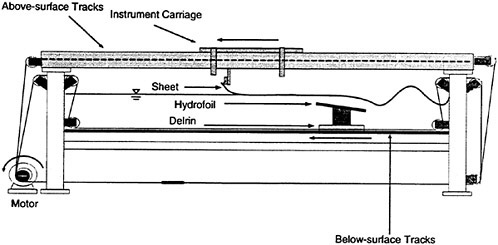
Figure 1: Side view of the towing tank.
2 Experimental Details
2.1 The towing tank
The experiment was performed in a towing tank with dimensions of 14.8 m long, 1.22 m wide and 1.0 m deep, see Figure 1. The sidewalls of the tank are made of glass to allow for flow visualization and optical measurements. The tank contains both below-surface and above-surface towing systems. The below-surface towing system includes two fully submerged ‘L’-shaped tracks that are mounted from the bottom of the tank near each of the long sidewalls. Objects are towed along the tracks by two stainless steel wire ropes which enter the water at one end of the tank and leave from the other end. Thus, no part of the towing system breaks the water surface in the vicinity of the towed object. The wire ropes are driven by a servo motor mounted at one end of the tank, see Figure 1. The above-surface towing system uses two tracks mounted above the tank, one near each sidewall. The above-surface towing system includes an instrument carriage which rides on the tracks via four hydrostatic oil bearings. When high-pressure oil is supplied to the bearings, a thin film of oil is forced between the bearings and the tracks, thereby greatly reducing vibration and friction levels of the carriage. The carriage is driven by two separate wire ropes which are powered by the same servo motor that powers the below-surface towing system. Precise towing speeds are obtained by means of a computer-based feedback control system.
In the present experiments, steady waves were generated with a hydrofoil mounted to the below-surface towing system. The hydrofoil is an aluminum NACA 0012 airfoil with a 20-cm chord which is operated at a 9° angle of attack. This foil spans the width of the tank with a small clearance of 1.4 cm between the edges of the foil and the walls of the tank. The foil is mounted to two stainless steel plates which, in turn, are mounted to two Delrin blocks, each with a groove cut into it. These grooves provide a low friction bearing surface to slide along the submerged L-shaped tracks. The surface wake was created with sheets of Mylar dragged along the surface of the water at a fixed distance ahead of the hydrofoil. The Mylar sheets have a thickness of 0.13 mm and a specific gravity of 1.25. Although these sheets are heavier than water, the contact angle at the Mylar-air-water interface around the edges of the sheet allowed the sheets to remain on the water surface. Two Mylar sheets were utilized, each having the physical dimensions as shown in Table 1.
Table 1. Physical dimensions of the short and long Mylar sheets.
|
|
short |
long |
|
length, cm |
63.5 |
101.6 |
|
width, cm |
101.6 |
114.3 |
|
contact length, cm |
56 |
94 |
The mounting assembly used to hold the Mylar sheets in place was attached to the above-surface carriage via two linear motion slides to allow for vertical positioning of the entire assembly. The relative position between the above-surface carriage and hydrofoil is adjustable. This allows the separation distance between the trailing edge of the Mylar sheet and the leading edge of the hydrofoil to be varied. Towed by itself, the sheet created a wake at the water surface and, as discussed below, a train of small-amplitude waves.
In order to control water clarity and surfactants, a recirculating skimmer system was used. This system
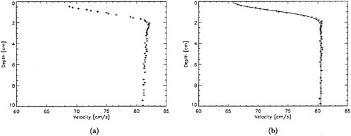
Figure 2: Mean horizontal velocity versus depth below the mean free water surface at a distance of 38 cm behind the trailing edge of the short Mylar sheet (no hydrofoil): (a) Raw velocity data; (b) Velocity data after subtracting Uw(z). The solid line is a least squares fit of Equation 5. Short Mylar sheet, X=38 cm.
includes two surface skimmers located at one end of the tank. The water from the skimmers was sent to a diatomaceous-earth filter and then sent back to the tank through a port at the opposite end of the tank from the skimmers. When fresh water was needed, tap water was sent through a separate filter before entering the tank. The skimming system was run for at least 2 hours before any measurements were taken.
2.2 Mean velocity measurements
A rake of three pitot tubes was used for the mean velocity measurements in the wakes of the Mylar sheets. The rake had a horizontal spacing between tubes of 10 cm and a vertical spacing of 10 mm. The large horizontal spacing was chosen to minimize the interaction between the individual tubes. The rake was mounted to a telescoping arm which was attached to the instrument carriage, allowing the stream-wise distance from the trailing edge of the Mylar sheet to the tips of the tubes to be varied. The Pitot tube rake was attached to the arm via a linear traverser to allow vertical positioning. Each Pitot tube was connected through transparent Tygon tubing to a separate differential, diaphragm-type pressure transducer (Validyne Model P305D), each having a range of ±0.2 psi. The three pressure transducers were mounted to the end of the telescoping arm at equal heights above the water surface. The analog voltage output of each pressure transducer was connected to a 12-bit analog-to-digital (A/D) converter operating at 1200 samples per second and the digitized output was stored in the memory of a PC. The signal taken during the steady state part of each run was then averaged. Division of the full pressure range of the transducer by the resolution of the A/D converter yields an accuracy of 0.1 cm/s at an average speed equal to the towing speed, 80.5 cm/s. However, during runs made with the Pitot tubes moving through the undisturbed water in the towing tank, a pressure fluctuation corresponding to a root-mean-square velocity fluctuation of 0.2 cm/s was observed.
The above-described equipment was used to measure the vertical distribution of mean horizontal velocity at three streamwise locations behind each Mylar sheet. These measurements were performed without the presence of the hydrofoil. In performing these experiments, it was observed that, like the hydrofoil, the Mylar sheets generated a train of two-dimensional surface waves. Though the amplitudes of these waves were small (at most 0.17 cm), they were found to have a noticeable effect on the mean velocity distributions (see below). In order to use the Pitot tubes in locations where the fluid velocity was known to be horizontal, the velocity distributions were measured at the streamwise locations of the troughs of the following wavetrain. Visual examination of the wavetrains showed the wavelength of the waves to be about equal to the difference in length of the two Mylar sheet (≈40 cm). The measurement locations were taken as 38, 80, and 120 cm behind the trailing edge of the short Mylar sheet and 40, 80 and 120 cm behind the trailing edge of the long Mylar sheet.
A mean velocity distribution at one streamwise
location was typically measured during the period of one day. A series of calibration runs was performed before and after each set measurements. During the calibrations, the Mylar sheet was removed, the carriage was run at a series of known speeds, and the resulting output from the pressure transducers was recorded. During each experimental run with the Mylar sheet, the streamwise and vertical positions of the probes were held fixed. For a given streamwise location, the measurement depths were varied in a random manner from run to run until measurements at enough depths were taken to ensure a well resolved profile of the mean velocity; runs at most measurement depths were repeated three times. The finite size of the Pitot tubes resulted in an inability to make fluid velocity measurements closer than about 5 mm from the water surface.
A sample of a raw mean velocity distribution is shown in Figure 2(a). In this figure, a depth of zero is the local free surface elevation. As can be seen in the plot the mean velocity increases slowly as the depth decreases from 10 cm to about 2 cm. Thereafter, the velocity decreases more rapidly to about 65 cm/s near the free surface. The increase in velocity between 10 and 2 cm in depth is an effect due to the small-amplitude wavetrain generated by the Mylar sheet. The horizontal velocity distribution in a potential flow wave at its trough can be described by linear wave theory (see for example [10]):
(3)
where z is the depth (positive down) relative to the mean water level, U∞ is the carriage velocity, a is the wave amplitude, k is the wavenumber given by ![]() in linear theory, and z is the depth below the mean water surface. The free surface is at z=−a. The above equation was fitted to the data by determining the wave amplitude that minimized the mean squared error over the depth range between 2<z<10. The resulting velocity profile, Uw, was then subtracted from all the data (0≤z≤10 cm). Several of the velocity distributions were also displaced by an amount Uos, where Uos≈−0.2 cm/s at most, to account for the fact that the distributions after subtracting out Uw did not asymptote to the known towing speed, U∞, see Section 3. The reason for this discrepancy between the asymptote and U∞ is not known. The final distribution after the above processing and displacing the profile upward by the wave amplitude, a, was called the wake velocity distribution and given the symbol U(z):
in linear theory, and z is the depth below the mean water surface. The free surface is at z=−a. The above equation was fitted to the data by determining the wave amplitude that minimized the mean squared error over the depth range between 2<z<10. The resulting velocity profile, Uw, was then subtracted from all the data (0≤z≤10 cm). Several of the velocity distributions were also displaced by an amount Uos, where Uos≈−0.2 cm/s at most, to account for the fact that the distributions after subtracting out Uw did not asymptote to the known towing speed, U∞, see Section 3. The reason for this discrepancy between the asymptote and U∞ is not known. The final distribution after the above processing and displacing the profile upward by the wave amplitude, a, was called the wake velocity distribution and given the symbol U(z):
where ![]() is the measured data. The wake velocity profile (U(z)) corresponding to the raw data in Figure 2(a) is given in Figure 2(b).
is the measured data. The wake velocity profile (U(z)) corresponding to the raw data in Figure 2(a) is given in Figure 2(b).
In order to obtain the surface velocity from the data and to have a mathematical form for the wake velocity profile, the final data U(z) was fitted to an equation given by
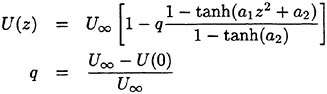
(4)
where a1 and a2 are fitting parameters. The best set of constants (U(0), a1 and a2) for the given velocity data set were determined by minimizing the sum of the squared deviations. (The tanh(a1z2) profile was used by [11] to fit the velocity profiles in the near wake of a hydrofoil and the tanh(a1z2+a2) profile was used by [12] in the near wake of a cylinder. In the present work, it was found that the latter function gives the best fit to the data.) A curve with form of Equation 5 with the computed constant set has been overlaid on the data in Figure 2(b). The above data processing was repeated for the three measurement distances for both Mylar sheets giving six velocity profiles (see Section 3).
2.3 Wave-height measurements
To measure the height of the incipient breaking waves created by the combination of the hydrofoil and the Mylar sheet, it was not possible to use wire gauges fixed to the tank because, in the towing tank, the Mylar sheet would collide with the gauge during the run. Thus, an optical wave-height gauge was used ([13]). In this device, the beam of a 5-Watt Argon-ion laser (Spectra Physics, model 2017) was pointed vertically down on the water surface at a fixed location in the wave tank. A pair of cylindrical lenses was used to convert the laser beam in to a light sheet that was one-mm thick and 8-cm long as it entered the water with the normal to the light sheet directed in the cross-stream direction. The water in the tank was mixed with Fluorescene dye at a concentration of about 1.5 ppm so that the water illuminated by the laser glowed with a greenish yellow color. The intersection of the laser beam and the water surface was observed via a digital linescan camera (Dalsa Lines-can Digital Camera Model CL-C4 2048A STDJ with a Nikon 200-mm lens). The camera was attached to a vertically oriented linear slide mounted onto a tripod that was fixed to the floor outside the tank. The camera viewed the wave from the side of the tank and
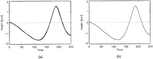
Figure 3: Wave-height profiles, (a) Profiles for four experimental runs with the same experimental condition, (b) Average of wave-height profiles in (a). Short Mylar sheet, Δxi=40 cm, d=26.4 cm.
above the waterline at approximately a 25° down angle; the plane defined by the line of sight of the camera and the single line of 2048 CCD elements (pixels) was oriented normal to the water surface and perpendicular to the center plane of the tank. At the plane of the light sheet the array of 2048 pixels covered a physical vertical distance of about 16 cm (0.08 mm per pixel). The CCD elements received little light from the air above the water surface but much more light from the glowing dye at the intersection of the laser light sheet and the water surface. The boundary between the poorly and brightly illuminated CCD elements was taken as the water surface. The camera was set up to record a single line of 2048 eight-bit pixels every 0.004 seconds. A total of 1.2 seconds of data was recorded during each experimental run creating an image (vertical distance versus time) of 2048 by 300 pixels. In each image, the water surface was located by an intensity-based thresholding technique. Before any images were taken, a calibration set was created by recording the position of the flat water surface with the camera set at five different heights above the water surface. These heights were known and repeatable through the linear positioner upon which the camera was mounted and gave the relationship between pixel position of the surface image and measured height. Before each set of experimental runs in measuring the waves, a single height image was taken with no wave present to determine the mean water level. In this run and in the calibration runs, it was found that the root-mean-square surface height fluctuation due to mechanical, electronic and data processing noise was about ±0.006 cm.
Each incipient breaking wave profile measurement began by taking an image of the undisturbed water surface to determine its position on the CCD array. Then the profile of the incipient breaking wave was measured in three independent experimental runs. A sample of the three wave profiles for a single experimental condition and the average of the three profiles is given in Figure 3. The wave height, ζ, was taken from the average profile as the vertical distance from the undisturbed water level to the wave crest.
3 Experimental Results
In this section the location of the incipient breaking conditions in terms of the external parameters of the experiment (foil depths and separations distances between the foil and the Mylar sheets) and the wake characteristics as a function of distance behind the trailing edge of the sheet are presented. These results along with the incipient breaking wave amplitudes are discussed in light of the numerical results and existing theory in Section 5.
3.1 Incipient breaking conditions
Incipient breaking conditions were determined visually through the following procedure. First the depth of submergence of the foil was fixed at a value for which, with no Mylar sheet, the wave did not break. Then the Mylar sheet was put in place and the horizontal separation distance, Δx, between the trailing edge of the Mylar sheet and the leading edge of the hydrofoil was set at a value small enough to cause
wave breaking. Over a series of experimental runs, Δx was increased. For large Δx the wake of the sheet at the location of the wave crest is very thick and has a very small surface drift. In this case, the wave behaves much like a wave in calm water, i.e., it does not break. Subsequent runs where used to locate the incipient breaking value of Δx, denoted as Δxi, which is defined such that for all Δx<Δxi the wave breaks. A plot of Δxi nondimensionalized by c (the chord of the foil) versus the depth of submergence, d, of the trailing edge of the foil (also nondimensionalized by c) is given in Figure 4. One curve for each Mylar sheet and six data points for each curve are given in the plot.
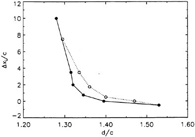
Figure 4. Incipient breaking conditions: separation distance between the trailing edge of the Mylar sheet and the leading edge of the hydrofoil, Δxi, versus the depth of submergence of the trailing edge of the hydrofoil, d, where c is the chord of the hydrofoil. Filled circles: short Mylar sheet, open circles: long Mylar sheet.
3.2 Wake characteristics
The wake characteristics (for instance the wake thickness and surface drift velocity) at the location of the incipient breaking wave crest must be determined from the wake velocity distributions which were measured at only three locations in each wake. Thus, characteristics of the mean velocity profiles must be determined by interpolation at places other than the three measurement locations. Three important characteristics of the wakes are the surface drift velocity,
(5)
the wake half-thickness, b1/2, where,
(6)
and the momentum thickness,
(7)
In the later analysis, the average values of θ for each Mylar sheet, θ=0.145 cm for the short sheet and θ=0.210 cm for the long sheet, are used. (The standard deviation for θ from the three measurements in each wake was only 3%.)
For a self-similar wake
(8)
Using a non-linear least squares method, the above equation was fitted to the six data points from the present data set. The resulting constants were C1=3.07 and x1=−47.98 and this curve is plotted along with the data in Figure 5(a). The variation of wake thickness can also be described by a similar power law defined by:
(9)
The constants resulting from a non-linear least squares fit to the data were C2=0.34 and x2=−74.78 and the data and the curve are shown in Figure 5(b).
4 Numerical Simulations
The interaction between the surface wake of the Mylar sheet and the gravity wave generated by the submerged hydrofoil is also studied numerically considering the following model of the process: the sheet wake is modeled as a two-dimensional, parallel shear flow, the hydrofoil wave is modeled as a plane, gravity wave, and the time evolution of their interaction is followed by numerical simulations of the Euler equations.
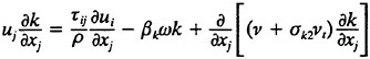
Direct numerical simulations (DNS) are used in non-breaking and incipient breaking conditions, while large wave simulations (LWS) are used for breaking conditions. In breaking conditions, the appearance of small scale free-surface fluctuations and overturnings on the face of spilling breakers prohibits the use of DNS. In LWS, only the large scale variables of the flow (velocities, pressure, free-surface elevation) are resolved, while the effect of small scales is modeled. In general, the resolved large scale, ![]() of a flow variable, f, is obtained by a spatial filtering operation,
of a flow variable, f, is obtained by a spatial filtering operation,
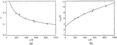
Figure 5: Surface drift velocity, q, (a) and Wake thickness, b1/2/θ, (b) versus measurement distance, x/θ.
which produces the following decomposition for every flow variable:
(10)
where f′ corresponds to the unresolved subgrid scale.
The velocity profile of the parallel shear flow is identical to the mean velocity profile measured in the wake of the Mylar sheet at a streamwise distance corresponding to the location where the free surface crosses the mean water level just upstream of the wave crest. As discussed above, the velocity profile of the shear flow is given by Equation 5. The plane gravity wave in the numerical model is a second-order Stokes wave with the appropriate wavelength, λ, according to linear theory:
(11)
The Froude number Fr of the flow, defined as
(12)
is related to the dimensionless wavenumber k of the gravity wave according to the following:
(13)
where the characteristic length scale b1/2 is the half-width of the velocity profile.
For the DNS of a two-dimensional, incompressible, inviscid, free-surface flow, the governing equations are the continuity equation
(14)
and the Euler equations
(15)
(16)
subject to the dynamic and kinematic free-surface boundary conditions, respectively,
(17)
where t is time, x, z are the cartesian coordinates (x is the horizontal coordinate, z is positive in the opposite direction of gravity, and z=0 corresponds to the mean free-surface level), u, w are the velocity components, p is the dynamic pressure, defined as the pressure P minus the hydrostatic pressure ![]() is the Froude number of the flow, and η is the free-surface elevation. In the above equations lengths are nondimensionalized by b1/2 and velocities by U∞.
is the Froude number of the flow, and η is the free-surface elevation. In the above equations lengths are nondimensionalized by b1/2 and velocities by U∞.
The free-surface elevation is an unknown function of time, which renders the flow domain time-dependent. Boundary fitted coordinates are introduced according to the following transformations:
(18)
(19)
where xi are the coordinates and ui are the velocity components in the transformed domain.
According to the above transformation, the continuity and the Euler equations, respectively, become
(20)
(21)
where
(22)
while the dynamic and kinematic free-surface boundary conditions, respectively, become
(23)
For the LWS, the governing equations are obtained by the spatial filtering of equations (20) and (21):
(24)
(25)
where the additional sub-grid scale (SGS) stresses ![]() contain the effect of the unresolved subgrid scales. The eddy SGS stress, τij, depends only on velocity interactions, while the wave SGS stress,
contain the effect of the unresolved subgrid scales. The eddy SGS stress, τij, depends only on velocity interactions, while the wave SGS stress, ![]() depends on the free-surface slope as well. The eddy SGS stress is the only term present in large eddy simulations (LES) of unbounded flows, while the wave SGS stress incorporates the free-surface influence. Both the eddy and wave SGS stresses are modeled using eddy-viscosity models (for details, see Dimas [14]). The dynamic and kinematic free-surface boundary conditions, respectively, become
depends on the free-surface slope as well. The eddy SGS stress is the only term present in large eddy simulations (LES) of unbounded flows, while the wave SGS stress incorporates the free-surface influence. Both the eddy and wave SGS stresses are modeled using eddy-viscosity models (for details, see Dimas [14]). The dynamic and kinematic free-surface boundary conditions, respectively, become
(26)
For both the DNS and the LWS of the Euler equations, an operator-splitting scheme is employed for the temporal integration and spectral methods for the spatial discretization with Fourier modes along the x1-direction, and Chebyshev polynomials along the x2 direction ([15]). Specifically for the DNS, 64 Fourier modes are used in the x1-direction, and 64 Chebyshev modes in the x2-direction, while the time step is 0.00025. For the LWS, a sharp Fourier cutoff filter is used to perform the filtering operation (10) where 24 Fourier modes are retained to represent the large scales of the flow; the other parameters are kept the same as in DNS. Periodicity boundary conditions are applied in the x1-direction, while the length of the computational domain in the x1-direction is equal to the wavelength of the gravity wave. Throughout the computation, Fast-Fourier-Transform algorithms are used to transform between physical and spectral space, and a spectral preconditioning technique is used on the pressure step of the splitting scheme, which renders the matrix of the resulting system of linear equations banded, thus dramatically reducing the computation time for its solution.
At time t=0, the computation starts with the mean velocity profile and the flow field of the plane gravity wave, while the initial free-surface elevation corresponds to the second-order Stokes wave with an initial wave amplitude ηmax.
For this paper, three velocity profiles are considered:
-
θ=1.4 mm, q=0.3, b1/2≈5 mm, Fr=3.60,
-
θ=1.4 mm, q=0.2, b1/2≈7 mm, Fr=3.06, and
-
θ=1.4 mm, q=0.1, b1/2≈13 mm, Fr=2.25.
For each velocity profile, the wavelength is evaluated according to (13), while several dimensionless wave amplitudes ηmax are considered. Results for q=0.3 are presented for Hmax=0.30, 0.34, 0.36 and 0.40, where Hmax is defined as:
(27)
where ηmαx=ζmax/b1/2. For the Stokes limiting wave, Hmax=1 (see Equation 1). The time development of the free-surface elevation for all four cases is shown in a frame of reference moving with the wave phase velocity in Figure 6. In each case, the free-surface shape is plotted every dt=5 time units, while for every new curve, the mean water level is shifted upwards by dη=0.5 from that of the previous curve. In all cases, after about t=20, the free-surface elevation becomes asymmetric about the wave crest, although the initial condition is symmetric. The level of asymmetry increases as Hmax is increased. For
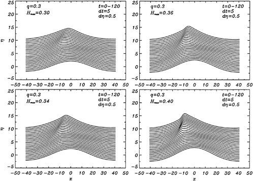
Figure 6: Time development of the free-surface elevation, η, for four different initial wave amplitudes, Hmax. In each case, the free-surface shape is plotted every dt=5 time units, while for every new curve, the mean water level is shifted upwards by dη=0.5 from that of the previous curve.
the highest value, Hmax=0.40, the free-surface elevation develops a bulge shape on the forward face. This shape is similar to that found in gentle short-wavelength spilling breakers (see [17]). The point of maximum upward curvature at the leading edge of the bulge is called the toe.
For cases with Hmax≥0.36, vorticity contour plots of the flow around the time of the bulge formation (at about t=80) exhibit an instability of the vorticity field. A typical example is shown in Figure 7 from the DNS of the case with Hmax=0.36. The instability is localized in the area of the toe at x≈−12 and is associated with the sharp variation of the free-surface slope which can not be resolved by a finite number of modes. On the other hand for cases with Hmax≤0.30, there is no bulge formation during the free-surface development and the vorticity distribution remains smooth. As discussed in the following section, these differences in the vorticity field are used to define incipient breaking conditions in the numerical results. For the breaking case with Hmax=0.36, the LWS filters out the SGS instability of the vorticity field (as shown in Figure 7) and successfully continues the computation past the breaking point. In fact at time t=140, the LWS shows the appearance of a vortex at the face of the breaker (see Figure 8) which may be associated with the formation of a shear layer in the wake of steady spilling breakers (Coakley [16]). To this end, further comparison with experimental data is necessary.
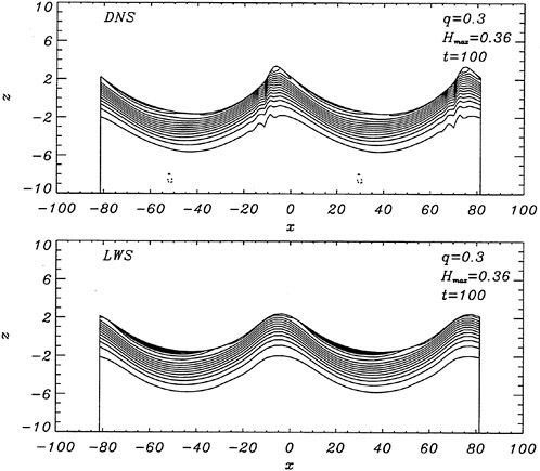
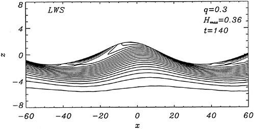
Figure 8: Vorticity contour plot from LWS calculation of the flow at a time instant after breaking. Solid contours correspond to negative vorticity, broken contours correspond to positive vorticity, and the increment between contours is 0.007.
5 Discussion
To examine the effect of the surface wake on the experimentally determined incipient breaking conditions, the dimensionless wave height, Hmax, is plotted versus the dimensionless drift velocity, q, in Figure 9. The values of ζmax were taken from the profile measurements at the 12 incipient breaking conditions plotted in Figure 4. The corresponding values of q were taken from Equation (8) with the measured value of θ for each wake and the streamwise location behind the sheet taken at the point where the water surface profile crossed the mean water level just upstream of the wave crest. (Varying this location back to the crest did not change the results significantly.) The values of q thus obtained are directly comparable to the definition of the surface drift in Banner and Phillips [6]. As can be seen from the figure, the experimental data for both the long and short Mylar sheets follow a single curve. This indicates that the variations in wake momentum thickness (for θ=0.145 cm and 0.210 cm or θ/λ=0.0035 and 0.0051, respectively) have little effect on the incipient breaking amplitude for the single towing speed used here, 80.4 cm/s. The data point plotted at q=0 is from Duncan [3] for a steady wave moving in calm water. Waves with amplitudes a little higher than this value will form a steady breaker if disturbed from equilibrium for a short time (see Section 1).
Also plotted in Figure 9 is a curve showing the theoretical result due to Banner and Phillips [6]. The shape of this curve is similar to that of the experimental data, but the magnitude is considerable higher. With this in mind, the theory of Banner and Phillips [6] is modified herein such that the incipient breaking condition is defined as the wave amplitude for which the fluid velocity at the crest is αU∞, where the factor α is to be determined from the experimental data. The resulting modified form of Equation 2 is
(28)
From a least squares fit to the experimental data (including the point from [3]), α was found to equal 0.50 and the resulting curve is plotted as a dotted line in Figure 9. This modified theory overestimates the wave height at q=0 but is otherwise a fairly good fit to the data. If this theory is assumed to be accurate, it would indicate that incipient breaking occurs in the presence of a surface wake when the fluid particle speed at the crest reaches 50 percent of the wave phase speed.
Our numerical simulations indicate that the time evolution of the fluid velocity at the crest reaches a minimum value during the bulge formation. As an example, for q=0.1 and Hmax=0.56, the time development of the fluid velocity magnitude, v=(u2+w2)1/2, along the free surface is shown in Figure 10. As can be seen from the figure, the fluid velocity magnitude at the crest reaches a minimum at about t=45 during the bulge formation. This minimum value of the crest fluid velocity is a function of the drift velocity, q, and the dimensionless parameter Hmax. For values of Hmax along the dotted line of Figure 9 the minimum crest velocity is not equal to 0.5U∞ as predicted by the modified theory of Banner and Phillips [6]. In fact, the minimum crest velocity
varies from about 0.3U∞ for q=0.1 to about 0.5U∞ for q=0.3. This difference between our numerical results and the theory of [6] arises from the fact that our model includes the unsteady nonlinear evolution of the wake layer and its vorticity field.
At incipient breaking conditions, an instability appears to develop at the toe of the wave as discussed in the previous section. For a given value of q, we define a range for the wave amplitude parameter Hmax in the following manner. The lower limit of the range corresponds to the maximum initial amplitude of the gravity wave for which no instability develops at the toe of the wave during the simulation, indicating no breaking. The upper limit of the range corresponds to the minimum initial wave amplitude for which a strong instability originates at the toe of the wave, indicating a definite breaking condition. These numerically determined boundaries are plotted in Figure 9 and are in good agreement with the experimental data.
6 Conclusion
The experiments and numerical simulations reported herein indicate that, as proposed by Banner and Phillips [6], the maximum amplitudes of steady nonbreaking water waves are reduced in the presence of a surface drift layer that flows in the direction of wave propagation, and the reduction increases with increasing drift velocity. Our results, though, indicate that these maximum heights are much smaller than the ones predicted by [6] whose breaking criterion is based on the assumption of zero fluid velocity at the wave crest in the frame of reference moving with the crest. For example, for the highest surface drift velocity used herein, q=0.27, our incipient breaking height is about 60% of the one predicted by Banner and Phillips [6] and about 33% of the Stokes’ wave limiting height. Our incipient breaking heights are independent of the wake momentum thickness over the range from θ=0.145 cm to 0.210 cm (λ/θ=286 to 197, where ![]() is the wavelength from linear theory in calm water). The numerical simulations show that breaking is associated with the formation of a bulge on the forward face of the crest of the wave and a point of high upward curvature (called the toe) at the leading edge of this bulge. For large enough wave steepness, it is observed that vorticity fluctuations increase dramatically just under the surface in this region of the flow. The incipient breaking amplitudes based on whether or not this local growth of vorticity fluctuations occurs are in good agreement with the experimental data.
is the wavelength from linear theory in calm water). The numerical simulations show that breaking is associated with the formation of a bulge on the forward face of the crest of the wave and a point of high upward curvature (called the toe) at the leading edge of this bulge. For large enough wave steepness, it is observed that vorticity fluctuations increase dramatically just under the surface in this region of the flow. The incipient breaking amplitudes based on whether or not this local growth of vorticity fluctuations occurs are in good agreement with the experimental data.
Through the experimental measurements of the surface drift velocity without the wave and the incipient breaking wave heights and theoretical analysis like that of Banner and Phillips (1974), it was found that the crest fluid velocity at the incipient breaking condition in the reference frame of the crest is 50% of the wave phase speed, U∞, relative to the water at infinite depth. Our numerical simulations, though, indicate that the fluid particle velocity at the crest for incipient breaking conditions varies from 0.3U∞ for lower drift velocities to 0.5U∞ for higher velocities. The difference between these values of the crest velocity and those from the experimental data/theoretical analysis mentioned above is assumed to be due to the inclusion of the unsteady nonlinear evolution of the wake layer and its vorticity field in the numerical calculations.
It is concluded, therefore, that the incipient wave height is lower than the one predicted by Banner and Phillips [6] due to the vorticity action in the toe region, which renders the use of a zero-crest-velocity criterion impractical to characterize incipient breaking conditions.
Acknowledgments
The support of the Office of Naval Research under contract N000149610368, Program Officer Dr. Edwin P.Rood, is gratefully acknowledged.
References
[1] Battjes, J.A. & Sakai, T. “Velocity Field in a Steady Breaker,” J. Fluid Mech., Vol. 111, 1981, pp. 421–437.
[2] Duncan, J.H. “An Experimental Investigation of Breaking Waves Produced by a Towed Hydrofoil,” Proc. R. Soc. Lond., Vol. 377, 1981, pp. 331–348.
[3] Duncan, J.H. “The Breaking and Non-Breaking Resistance of a Two-Dimensional Hydrofoil” J Fluid Mech., Vol. 126, 1983, pp. 507–520
[4] Parker, F. “The Royal Navy’s Boxer,” Proceedings of the U.S. Naval Institute, Vol. 120, 3, 1994, Cover.
[5] Stokes, G.G. “On the Theory of Oscillatory Waves,” Trans. Camb. Phil. Soc., Vol. 8, 1847, pp. 441.
[6] Banner, M.L. & Phillips, O.M. “On the Incipient Breaking of Small Scale Waves,” J. Fluid Mech., Vol. 65, 1974, pp. 647–656.
[7] Simmen, J.A. and Saffman, P.G. “Steady Deep-Water Waves on a Linear Shear Current,” Studies in Applied Mathematics, Vol. 73, 1985, pp. 35–57.
[8] Teles Da Silva, A.F. and Peregrine, D.H. “Steep, Steady Surface Waves on Water of Finte Depth with Constant Vorticity,” J. Fluid Mech., Vol. 195, 1988, pp. 281–302.
[9] Salvesen, N. and von Kerczek, C. “Nonlinear Aspects of Free-Surface Flow Past Two-Dimensional Bodies,” 14th IUTAM Delft, 1976. See also Salvesen, N. “Five Years of Numerical Naval Ship Hydrodynamics at DTNSRDC,” J. Ship Research, Vol. 25, 4, 1981, pp. 219–235.
[10] Lamb, H. Hydrodynamics, Dover Press, 1932.
[11] Mattingly, G.E. & Criminale, W.O. “The Stability of an Incompressible Two-Dimensional Wake,” J. Fluid Mech., Vol. 51(2), 1972, pp. 233–272.
[12] Triantafyllou, G.S., Triantafyllou, M.S. and Chryssostomidis, C. “On the Formation of Vortex Streets Behind Stationary Cylinders,” J. Fluid Mech., Vol. 170, 1986, pp. 461–477.
[13] Lin, J.-T. & Liu, H.-T. “On the Spectra of High-Frequency Wind Waves,” J. Fluid Mech. Vol. 123, 1982, pp. 165–185.
[14] Dimas, A.A. “Large Wave Simulations (LWS) of Free-Surface Flows,” Proceedings, ASME Fluids Engineering Division Summer Meeting FEDSM97–3408, 1997, pp. 1–6, Vancouver, Canada.
[15] Dimas, A.A. “Free-Surface Waves Generation by a Fully-Submerged Wake,” Wave Motion Vol. 27, 1998, pp. 43–54.
[16] Coakley, D.B. and Duncan, J.H. “The Flow Field in a Steady Breaker,” Presented at the 21st Symposium on Naval Hydrodynamics, 1996, Trondheim, Norway.
[17] Duncan, J.H., Qiao, H., Behres, M. and Kimmel, J. “The Formation of a Spilling Breaker,” Physics of Fluids, Vol. 6, (8), 1994, pp. 2558–2560.
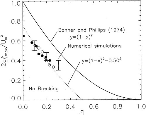
Figure 9: Non-dimensional wave amplitude versus local drift velocity at incipient breaking conditions: Filled circles—short Mylar sheet; open circles—long Mylar sheet; filled square—data from Duncan (1983); solid line—theory of [6]; dotted line—modified theory (see Equation 28). The bars are from the present numerical calculations: top horizontal line is definitely unstable, bottom horizontal line is definitely stable.
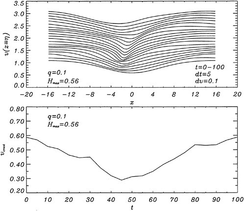
Figure 10: Time development of the free-surface fluid velocity magnitude (upper plot) and the crest velocity magnitude (lower plot). In the upper plot, each curve is plotted every dt=5 time units and it is shifted upwards by dv=0.1 from the previous curve.
DISCUSSION
T.Sarpkaya
Naval Postgraduate School, USA
It seems to me that this is an investigation of the introduction and alteration of the free-surface vorticity distribution on (or near) the surface of a small amplitude laminar wave. Also the analysis (of Dimas) used by the authors is only that of an inviscid wave (Euler’s analysis) with a free-surface shear layer. In view of the foregoing, I have the following questions: (1) How will the use of different Mylar sheets (thickness, weight, roughness, porosity) affect the measurements, wave breaking and its location since they will undoubtedly introduce different amounts of vorticity?, (2) How is the problem investigated related to the problem of the incipient breaking of turbulent waves generated by a ship and the vorticity manipulation of the free-surface of such highly turbulent waves?, (3) Does the problem need a turbulent numerical model and similar turbulent wave breaking experiments to bring the objectives of the investigation closer to what is investigated?
AUTHORS’ REPLY
(1) Thus far, we have only performed experiments with surface wakes generated by two smooth Mylar sheets of different lengths. The results obtained indicate that the incipient breaking wave heights correlate with the surface drift velocity while being independent of wake momentum thickness. Thus, the present results would indicate that the different types of Mylar sheets mentioned by Prof. Sarpkaya, would only affect the results to the extent that they change the streamwise position of a given surface drift velocity behind the sheets. Verification of this conjecture will have to await further experimental results. (2) The present work is intended as a two-dimensional model of the
ship wave problem. The waves at the stern are generated primarily by the displacement effect of the hull and this is accounted for by the hydrofoil in the present experiments. The surface wake found upstream of the stern wave is composed of both the boundary layer of the hull and the wakes of breaking waves at the bow. In both the ship waves and the present experiments, the wakes are turbulent and the breaking waves, when they occur are, of course, turbulent. The main differences between the two cases are that the Reynolds number and Weber number are higher for the ship flow field and that the ship wave mean flow field is three dimensional while the mean flow field is two dimensional in the present experiments. These differences are certainly significant and need to be explored. (3) We think that the good agreement between the measured and computed incipient breaking wave amplitudes indicates that the turbulence has only a small effect on this aspect of the flow. However, once the wave is breaking, we believe that a turbulence model is essential for computing quantities like the breaking wave drag and the surface mixing. Further development of the three-dimensional Large Wave model described in the paper is intended to simulate these breaking waves.
DISCUSSION
B.Johnson
U.S. Naval Academy, USA
-
Please characterize the Reynolds numbers at the end of the various Mylar sheets.
-
The naval ship photograph with a large breaking wave just beyond the stern (presented in the talk but not the paper) is probably caused by the large vorticity associated with the transom stern separation. Did you vary the depth of the boundary layer generator to show the effects of the large scale vorticity?
-
Very well done and well presented paper.
AUTHORS’ REPLY
1. The Reynolds numbers based on the towing speed and the wetted lengths of the short and long Mylar sheets were 450,800 and 756,700, respectively. The appearance of random patterns of ripples on the water surface downstream of the sheets is a clear indication that the wakes are turbulent. 2. We also suspect that the breaker behind the stern of the ship in the photograph is strongly affected by the vorticity shed by the hull. At this point in time, we have only used the floating Mylar sheets to generate a surface boundary layer. We had not thought of exploring the effect of a submerged wake generator on the breaking criterion. Thank you for an interesting idea.
DISCUSSION
K.-h.Mori
Hiroshima University, Japan
The inclusion of the turbulent characteristics is crucial for the numerical simulation of such type of breaking as dealt with in the paper. It may sometimes provide different wave profiles from those computed without. Could you have some results which demonstrate the effects of the turbulence? And what are the turbulent quantities at the crest? By the way, the tangential condition on the free surface is important when the turbulence is taken into account. How did you deal with the tangential condition?
AUTHORS’ REPLY
In our numerical simulations of the incipient breaking conditions, we approximated the wake as an inviscid, initially laminar shear layer. The numerically computed wave heights found at the incipient breaking conditions agree well with those found experimentally. The incipient breaking wave heights in both the experiments and the numerical results correlate with the surface drift velocity and are independent of the wake momentum thickness (at least in the range of wake momentum thicknesses studied). Given the agreement between the numerical model and the experimental results, we suspect that the effect of the turbulence in the wake of the Mylar sheet on the incipient breaking condition is primarily as the perturbation that triggers the transition from a nonbreaking to a breaking wave. Once the wave is breaking, a turbulence model is needed for both the flow and the free-surface fluctuations. In this paper, the Large Wave model is applied on an inviscid flow; therefore, the free surface is assumed to be stress-free. The development of Reynolds stresses is based exclusively on the cascade of instabilities to small scale fluctuations. Viscous effects are not expected to change the incipient breaking conditions but may alter the post-breaking behavior and will be considered in the future. In the experiments, at this point in time, we have not made measurements of the fluctuating flow field under the free surface.
Computation of Ship Wake Flows with Free-Surface/Turbulence Interaction
M.Hyman (Coastal Systems Station, Panama City, USA)
Abstract
It has long been evident that some process which enhances near-surface spreading is active in the evolution of surface ship wakes. Comparison of full scale data with results from CFD simulations indicate that by far the largest error in the simulations is due to too slow lateral growth at the free surface. Since the simulations are based on Parabolic Navier-Stokes solvers, several possible reasons for the error have been suggested, including incorrect upstream boundary conditions, errors introduced by neglecting free surface deformation (Froude number effects) and the modification of turbulence by the free surface. In the present discussion, it is suggested that correct inclusion of a relatively simple free-surface/turbulence model leads to dramatic qualitative improvements in near-sur-face lateral wake growth. It is also shown that the interaction is confined to a relatively thin layer near the free surface which must be resolved if numerical simulation of the wake is to be successful.
Introduction
Attempts to numerically model surface ship wakes by solving ensemble-averaged equations over the past 10 or so years have had mixed success. Here, “wake” refers to flow at all distances astern the ship, near the ship track. The near wake refers to the hydrodynamic and passive scalar fields from 0 to 1 length astern the ship and the far wake refers to these quantities between 1 and 20 (or more) ship lengths astern the ship. In general, the main features of the wake can be reproduced, but one feature that has persistently defied explanation is the slow lateral growth, near the free surface, of wakes computed by numerical models as compared to observations of full scale wakes. Reed, et. al. (1), suggest that the spreading is due to bilge and stern vorticies. Innis (2) alludes to this problem and suggests possible explanations. Hyman, (3) also discusses it and notes several sources of error inherent in the numerical models and methodology which may contribute to the lack of agreement. He notes that inclusion of bilge vorticies in far wake calculations produce wake spreading but also deep side lobes which are not commonly observed in full scale acoustic data.
Far wake simulations rely on parabolic Navier-Stokes (PRaNS) solvers. These solvers are fast and can be shown to be an extremely good approximation to the full elliptic RaNS equations in the far wake. Since the equations are parabolic, a set of flow data in the near wake is required to initiate a calculation. The simulations are typically performed under the assumption that the free surface deformation has little or no effect on the wake and particularly on the transport of passive scalars in the wake (such as temperature, salinity or microbubbles). Furthermore, since the equations are ensemble-averaged, models for the Reynolds stresses and velocity-scalar correlations are required. All of these assumptions or restrictions are possible sources of error.
The most obvious source of error is the first point noted above—specification of data in the near wake. We label this the Initial Data Plane (IDP). The data reflects the mean flow, turbulent field and scalar fields that exist in the near wake. The discussion in Hyman, (6) shows that this plane can be as close as half a ship length astern the ship and still satisfy the assumptions implicit in the PRaNS equations. These are difficult data to acquire either experimentally or numerically, particularly for a wide variety of ship geometries over useful ranges of operating conditions. In general, the data have been estimated by imposing conservation of momentum and mass and utilizing generic wind tunnel and tow tank data. Methodologies for these calculations can be found in Miner, et al. (4) and Hyman (5). More recently, Hyman (6), Reynolds averaged Navier-Stokes algorithms that can be used to compute data at the IDP have been developed. These algorithms, which compute the flow around the ship and into the near wake, also include a nonlinear free surface boundary condition in order to allow the computation of the deforming free surface and the Kelvin wake. One of these, reported in Tahara and Stern (7) and Stern, et al., (8) has been modified to include the calculation of the development of nonuniform ambient temperature and haline fields around the ship and in the wake. This algorithm has been used to compute the IDP (see Paterson, et al. (9)) around a wide variety of hulls and for wake simulations.
The work in Hyman (6) suggested that it is improbable that slow near surface wake growth is due to errors in IDP specification. No feature could be seen in any of the calculations that resembled the near surface vorticity which seems to be associated with near surface spread-
ing. Of course, the calculations on which that conclusion was based could be in error. In addition, a study that included free surface deformation in the wake simulation (both at the IDP and downstream), also in Hyman (6), indicates that surface waves or wave driven currents are not responsible for the spreading.
At this point one is left with the conclusion that surface spreading is likely to be due to free surface/turbulence interaction. Attention has been given to the interaction of turbulence with the free surface for some time. Shir, (10) proposed a model for the redistribution of turbulent strains due to interaction with solid surfaces. Komori and Ueda, (11) and Ueda, et al., (12) measured turbulence quantities near the free surface in channel flow. They modeled the effect of the free surface as driving the eddy diffusivity to zero. Celik and Rodi, (13) cast Shir’s framework into a k-epsilon model and used it to compute 2-D turbulent channel flows.
In an effort to understand the interaction, work reported in Walker, et al., (14) and Walker, (15) was undertaken to study a near-surface jet at several Froude numbers. Walker and Chen, (16) used experimental data to evaluate terms in several algebraic stress models, including one similar to that suggested by Shir, (10), and found that they could not develop sufficiently strong anisotropy near the surface. Sreedhar and Stern, (17) successfully used a nonlinear k-epsilon model with free-surface damping within a RaNS algorithm to reproduce observed outward, near-surface currents near a surface piercing flat plate. As a result of the above efforts, the unsuccessful attempt at using the model Celik and Rodi, (13) in Hyman, (3) on ship wakes was revisited. The present report discusses the results of that and related work.
General Features
It has been recognized for some time that the free surface has an influence on turbulence development and the literature on the subject has become quite extensive. Some of the work has been of a more fundamental nature, vortex connexions etc. and of greater relevance to workers in LES or DNS. Of more interest to the present problem is the work by Anthony and Wilmarth, (18), Swean, et al., (19), Swean et al. (20), Miner, et at. (21) and Walker et. al. (14) in which the general characteristics of turbulence in jets near a free surface are investigated. It has become apparent that the vertical turbulent strains ![]() are damped in the neighborhood of the free surface and that the energy contained in these fluctuations is redistributed to the other two components. The work by Rood, (22) suggests that the overall turbulent kinetic energy is reduced near the free surface. Thus simultaneously, the energy is decreasing and the anisotropy is increasing as the free surface is approached. In addition, it appears that the isotropic component of the energy dissipation rate is likewise damped as the free surface is approached. These features seem to stimulate, or are associated with, a lateral current (Walker, (15)), immediately below the free surface. This current is also associated with a region of high streamwise vorticity although it would be incorrect to characterize the flow structure as a vortex. Both Walker, (15) and Sreedhar and Stern, (17) show that the controlling term driving the surface current is the anisotropy between the lateral and vertical strains.
are damped in the neighborhood of the free surface and that the energy contained in these fluctuations is redistributed to the other two components. The work by Rood, (22) suggests that the overall turbulent kinetic energy is reduced near the free surface. Thus simultaneously, the energy is decreasing and the anisotropy is increasing as the free surface is approached. In addition, it appears that the isotropic component of the energy dissipation rate is likewise damped as the free surface is approached. These features seem to stimulate, or are associated with, a lateral current (Walker, (15)), immediately below the free surface. This current is also associated with a region of high streamwise vorticity although it would be incorrect to characterize the flow structure as a vortex. Both Walker, (15) and Sreedhar and Stern, (17) show that the controlling term driving the surface current is the anisotropy between the lateral and vertical strains.
It seems clear that near surface anisotropy must develop and will stimulate an outward surface current. There may be additional effects, such as dissipation of energy via wave radiation, that also influences the near-surface turbulence evolution.
Mathematical/Numerical Model
Near Field
As noted above, flow data in the near wake must be obtained before the far wake computation can begin. This data is generated by solving the full RaNS equations to determine the flow around the ship and into the near wake. The CFDSHIP-IOWA RaNS solver is used for this calculation. Although the algorithm can be used to to compute the flow with or without free surface deformation, in the present application, the free surface is not allowed to deform. This choice is made as a result of the observation, alluded to above, that including free surface deformation in the near wake does not play a role in the far wake development.
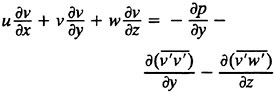
The unsteady RaNS and continuity equations for an incompressible fluid, written in non-dimensional form and Cartesian tensor notation are:
1
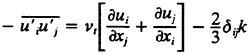
2
where ui are mean velocity components and xi are Cartesian coordinates, p is piezometric pressure, ![]() are the Reynolds stresses and
are the Reynolds stresses and ![]() are the body force terms which are used to model the effects of a propeller.
are the body force terms which are used to model the effects of a propeller.
Closure is obtained via the following relationships;
3
In the present work, the Reynolds stresses are specified using the blended k-omega/k-epsilon model of Mentor (23):
4
5
6
for the near wall region and
7
8
in the region distant from the wall and in the wake. In equations. 7 and 8, the variable ∈ used in the k-epsilon equations has been transformed into the variable ω to simplify the blending. Experience has shown that this model exhibits good convergence characteristics over both the wall bounded and free shear regions of the flow.
Constants used in the model are as follows:
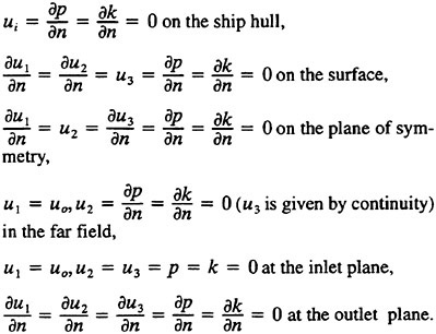
These equations are solved with boundary conditions as follows;
Far Field
The far field PRaNS equations are given below in Cartesian coordinates;
9
10
11
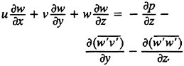
13
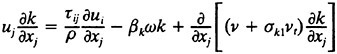
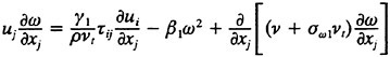
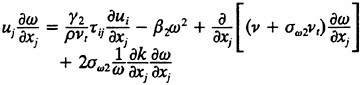
for incompressible, constant density flow. The turbulent stresses and strains are modeled with either the linear k-epsilon model or the algebraic stress model (ASM) of which the k-epsilon model (KEM) is a component. In the far wake, we see only small differences in results obtained via the two models and, since the ASM is the more expensive of the two to compute, rarely use it. On the other hand, much more control over the turbulent stresses can be exerted with the ASM and so it is the model of choice in the present work. The k-epsilon equations to be used are:
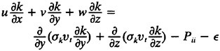
14
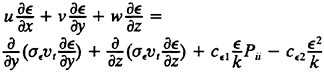
15
where ![]() . The stresses then are given by
. The stresses then are given by
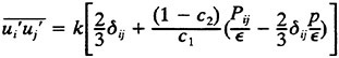
16
In the algorithm, the mean flow equations are first solved using the isotropic eddy viscosity from KEM, then the KEM equations are solved. Upon solution of the KEM equations, the ASM equations are solved via iteration, i.e., they are not cast in implicit form. At this stage we have the isotropic eddy viscosity and the turbulence stresses. We solve the momentum equations with the isotropic eddy viscosity as the implicit diffusion term and then in the source term subtract it back out (using the most recent estimate of the mean velocity field to calculate the velocity gradients) and also subtract out the turbulent stress gradients in equations 10–13.
Near the free surface, the model of Shir, (10) is used to impose anisotropy on the turbulent strains. With this model, equation 16 becomes;
17
with ![]() . This is a damping function that gradually increases the imposed anisotropy as the free surface is approached. In addition to the change in turbulent stresses, the dissipation rate is altered and becomes aniotropic. The dissipation is now given by;
. This is a damping function that gradually increases the imposed anisotropy as the free surface is approached. In addition to the change in turbulent stresses, the dissipation rate is altered and becomes aniotropic. The dissipation is now given by;
18
The function F is given by; ![]() . We choose the length scale to be equal to the energy-containing length scale
. We choose the length scale to be equal to the energy-containing length scale ![]() .
.
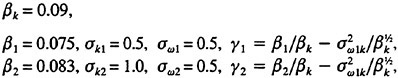
Constants used in the model are as follows; Cμ =0.09, σk=1.0, σ∈=1.3, C∈1=1.44, C∈2=1.92, C1=2.2, C2=1.5, Cs=0.6
These equations are solved with the same boundary conditions used in the RaNS equations noted above. They are solved with an implicit, second order finite difference scheme using a multistep, conjugate gradient solver.
Application
The algorithm is used to simulate two flows. The first is the computation of the flow behind a submerged jet Walker, (24). This is an attractive application because a submerged jet is similar to the wake of a high speed ship since these wakes are typically momentum excess flows. This is due to the fact that the thrust generated by the propellers greatly exceeds the skin friction drag, the difference being wave energy that is not found in the wake region in which we are interested.
The second application is the computation of the wake behind a propelled surface ship. The platform used is the model 5415 hull, a test hull form for RaNS flow development and validation. This twin propeller hull contains most of the features that are found in naval combatant hulls including bow domes, skegs and a transom stern.
Submerged jet
The submerged jet of Walker (24) is at a depth Froude no. of 8 and a Reynolds no. (based on diameter) of 11400. The jet is issuing from a nozzle 2 diameters below the surface and is measured at three locations downstream; 8, 16 and 32 diameters from the exit. The mean flow and the turbulence correlations, ![]()
![]() and k were measured on the three planes. These quantities, at the nearest plane, were used to create a data set (IDP) suitable for PRaNS algorithm initiation. The quantity that was not available was the dissipation rate. This was estimated from the length and velocity scales in the flow. The calculations suggest that better performance may be attained if the initial estimate of dissipation rate was optimized to some degree. Contour plots of mean flow variables at the plane 8 diameters downstream are shown in figure 1. The grid used in the computation is rectangular but nonuniform, with the highest density at the centerline and surface. The grid size is 50×199×99 in the axia, lateral, and vertical directions respectively. The computational domain was extended out to 20 jet diameters in the lateral and vertical directions. The ninimum grid spacing in each of these directions is 0.03 diameters. The axial grid was also nonuniform, with an initial spacing of 0.05 diameters and was extended to 24 diameters downstream.
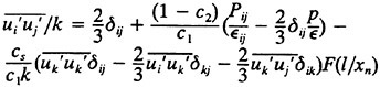
and k were measured on the three planes. These quantities, at the nearest plane, were used to create a data set (IDP) suitable for PRaNS algorithm initiation. The quantity that was not available was the dissipation rate. This was estimated from the length and velocity scales in the flow. The calculations suggest that better performance may be attained if the initial estimate of dissipation rate was optimized to some degree. Contour plots of mean flow variables at the plane 8 diameters downstream are shown in figure 1. The grid used in the computation is rectangular but nonuniform, with the highest density at the centerline and surface. The grid size is 50×199×99 in the axia, lateral, and vertical directions respectively. The computational domain was extended out to 20 jet diameters in the lateral and vertical directions. The ninimum grid spacing in each of these directions is 0.03 diameters. The axial grid was also nonuniform, with an initial spacing of 0.05 diameters and was extended to 24 diameters downstream.
Figure 1 shows that at 8 diameters, the jet axial velocity field looks similar to a jet exiting into an unbounded domain. The crossflow velocity field shows considerable influence of the free surface. Noticeable asymmetry exists in the vertical plane with a set of counter-rotating vorticies near the jet bottom and pronounced upward velocities near the surface. These fields were interpolated onto the PRaNS grid described above and used as initial data for calculations.
Results
While calculations were performed with several turbulence models, the ones presented here were obtained using the algebraic stress model noted above with the free surface model turned on. The results are presented in figures 2–5. These figures show measured and computed flow quantities at each of the downstream planes on opposite columns for ease of comparison. At the plane 16 diameters downstream of the exit, shown in figures 2 and 3, it is apparent that significant lateral near-surface spreading is taking place in the measured data. It is especially apparent in the plot of axial vorticity which shows a very thin layer of vorticity on each side of the centerline that is much wider than what might be discerned from the axial velocity field alone. A similar development is beginning in the calculations but to a much less pronounced degree. Axial vorticity is concentrated at the surface but has not spread laterally. The calculated vorticity is approximately a factor of 3 smaller than the measured vorticity. Plots of measured turbulent strains in figures 4 and 5 show that that there is little obvious influence of the free surface on these quantities at this location. The calculations also reflect this. It should be noted that the calculated velocity and strain fields are all significantly smaller in spatial size that the measured fields.
At 32 diameters downstream of the exit, the measured data show significant influence of the free surface on flow development. As at the previous plane, there is
a thin layer near the surface of vorticity on each side of the centerline. At this plane, the vortical layer is accompanied by the fluid with excess axial velocity. The calculated data show a significant spreading at the surface, though not to the degree present in the measured data. In addition, as in the measurements, nearly all the calculated vorticity is in a layer near the free-surface.
Both the measured and calculated turbulent strains at this plane display the anisotropy near the surface that has now become associated with turbulence/free-surface interaction. However, both computed strain fields are approximately 50 percent narrower than the measured fields.
While the spatial growth of axial velocity and turbulent kinetic energy of the computed flow is significantly slower than measured, the decay rate of axial velocity and the turbulent strain rates is closer.
Scrutinity of the decay plots of the variables of interest shed additional light on the modeling. Figures 6a and 6b show that the model captures the decay of maximum axial velocity and turbulent strains quite well. This was anticipated in the analysis of Walker and Chen, (14). It does not, however, capture the evolution of crossflow velocity maxima. The behavior of this variable is interesting. While the development of the measured maxima is not clear due to widely spaced measurement planes, the development of the computed maxima is such that it decreases until x/d of about 16 (the second measurement plane) and then monotonically increases. It is at this location that significant interaction between the strain field and the free surface begins to take place. This interaction, while modest in the computed solution, dominates the crossflow velocity field.
Ship Wake
In order to determine the effect of including a free-surface/turbulence interaction on ship wake development, the wake of a propelled model 5415 was computed. This geometry is presently a standard RaNS algorithm test geometry and is currently being used extensively in both calculation and measurement programs. A plot of the hull grid is shown in figure 6. The flow around this hull was computed with a relatively coarse, 2 block H-type grid, different from that used in test cases for this hull. The grid is 125×70×60 in block 1 and 100×70×60 in block 2. The flow was computed at Fr=0 so the computational domain was extended only to 0.5 L in the lateral and vertical direction. The domain and grid density were chosen to allow clustering of grid points in the region near the propellors and to provide better grid resolution in the wake, which here is our primary interest. A better solution would be to construct a separate block around and behind the propellor. The Iowa RaNS code is capable of this but time did not allow us to pursue that strategy. The calculation was performed at a Reynolds number of 15.6 million. The error in hull wetted surface area coefficient of the gridded model is 0.17 percent.
The propellor is modeled as an axisymmetric actuator disk using the methodology of Hough and Ordway. The actuator disk is intended to provide sufficient momentum to reproduce self-propulsion for the model scale hull at a Fr=0.27. The propeller has nondimensional diameter of 0.0182 and is operating at: j=1.27, KT=1.77 KQ=0.049.
It is not the purpose of this discussion to scrutinize the near ship flow. Instead, our interest is in the wake. Accordingly, figure 7 is presented which shows the axial velocity, axial vorticity and kinetic energy fields at 0.5 ship lengths (L) astern the aft perpendicular. This data is used at a starting solution to the far wake calculation. It shows a thin momentum-defect wake and a strong momentum-excess wake associated with the propellors. The maximum nondirectional axial velocity at this downstream location is 1.77 and the minimum is 0.53. The maximum crossflow velocity is in the swirling propeller jet and has a value of 0.11.
The PRaNS grid has size 200×200×100 in the axial, lateral and vertical directions. As in the previous case, the grid has highest resolution near the IDP, the surface and the centerline. The domain is extended out to 0.4 L in the lateral and vertical directions and to 10 L in the axial direction. The grid spacing is less than 0.001 L near the surface-centerline. The solution is less sensitive to lateral grid resolution and quite sensitive to resolution near the surface. As was apparent in the near-surface jet case discussed above, a thin layer develops near the surface that must be resolved.
Results
The 5415 wake was computed using the algebraic stress turbulence model with (ASM/FS) and without (ASM) near-surface anisotropy to provide a means of evaluating the effect of forced anisotropy. Figures 8 and 9 show the mean flow and strain fields computed using the baseline ASM model. The axial vorticity field is dominated by the propeller-induced swirl which gives rise to a pair of secondary vorticies below them. At greater distances downstream, these secondary vorticies, being below the region of highest turbulent viscosity, become stronger relative to the primary vorticies. At 10 L, most of the vorticity is found in the deep wake. The most obvious feature in these plots is the very slow lateral growth of the wake. Most of the width growth takes place in the first several lengths and then slows significantly. That, however, is not what one observes in field data. It is this deficiency that has led to speculation of the existence of streamwise vorticies near the surface that stimulate lateral wake growth.
The same calculation performed with the free-surface/turbulence interaction model, shown in figures 10 and 11 show a much different picture. While the overall
strains are nearly the same as computed with ASM only, at 5 L downstream, the vorticity near the free surface is a factor of 5 larger. In addition, the largest vorticity is found near the free surface rather than in the deep wake. This increase leads to a dramatic increase in surface wake width—which is larger by a factor of nearly 2. At 10 L downstream, the near-surface vorticity is larger by a factor of nearly 10 and surface wake width is more that twice that seen in the calculations with ASM only. At this plane, as at the 5 L plane the overall strains are approximately the same, but the FSF effectively drives the vertical strain to zero.
It must be noted that these effects cannot be obtained unless the near surface is sufficiently well resolved. The thickness of the near-surface layer is dependent on the form of the damping function, equation 19. This form is different from that used by Sreedhar and Stern (18) and will result in a thinner layer.
The differences between the model performance between the two cases is large. Since there exists little comparison data in ship wakes, it is not clear whether the model results reproduce these flows well. Certainly, the qualitative improvement is significant. From these results, it appears likely that wake spreading is due to near-surface vorticity generated by turbulent strain anisotropy rather than by bilge vorticies or other mean flow features created by the ship itself.
Including the interaction model in the RaNS algorithm used to generate the IDP would be very interesting. It is likely that even over the relatively short near wake region, there is sufficient time for anisotropy to alter the flowin the near wake and thus the IDP’s used to initiate far wake calculations.
Conclusions
The PRaNS model only was used to compute the development of the near-surface jet of Walker (24). The results indicate that the free-surface/turbulence interaction model does force anisotropy at the free surface and leads to enhanced spreading. Comparison with the measured data suggests that the modeled interaction is too mild and that the lateral growth rate remains too slow.
A RaNS/PRaNS algorithm has been used to investigate the influence of an algebraic stress turbulence model with free-surface/turbulence interaction on near-surface flow development. The effect of the interaction model on ship wakes is profound. Inclusion of this model leads to large increases in near-surface vorticity and significant increases in near-surface wake width growth. This is qualitatively correct but no published data is available to determine if it is quantitatively correct. A preliminary conclusion that significant differences exist beteween the two cases may be misleading since the simulations are taking place over vastly different scales.
An additional observation that might be made is that the sensitivity to the calculations of the form of the decay function should be determined. Differences between the forms used by Shir (10) and those used by Sreedhar and Stern (18) should be resolved. Walker and Chen (14) suggest that the functional form applied in the present work produces too thin an interaction layer. This might be the reason for the modeled data not well reproducing the observations.
Acknowledgements
This work has been supported by the Office of Naval Research, Code 333 under the direction of Dr. Edwin Rood and Ms. Sharon Beerman-Curtin. This support is gratefully acknowleded.
References
1. Reed, A.M. Beck, R.F., Griffin, O.M., and Peltzer, R.D. “Hydrodynamics of remotely sensed surface ship wakes”, SNAME Trans., 98, pp. 319–363. 1990.
2. Innis, G.E., “Computation of Full-Scale Wakes from Model-Scale Data”, SAIC-93/1139, July. 1993.
3. Hyman, M., “Modeling Ship Microbubble Wakes”, CSS/TR-94/39, August. 1994.
4. Miner, E., Ramberg, S., and Swean, T., “A Method for Approximating the Initial Data Plane for Surface Ship Wake Simulations”, NRL Memorandum Report, 6376, November, 1988.
5. Hyman, M., “Initial Data Plane Estimation for Surface Ships—II”, NCSC TN 930–88, July, 1988.
6. Hyman, M., “Calculation of Initial Data Planes for Ship Wake Simulations”, CSS/TR-96/07, November, 1996.
7. Tahara, Y. and Stern, F., “A Large-Domain Approach for Calculating Ship Boundary Layer and Wakes for Nonzero Froude Numbers”, Proceedings of CFD Workshop Tokyo, Mar., 1994.
8. Stern, F., Paterson, E. and Tahara, Y., “CFDSHIP-IOWA: Computational Fluid Dynamics Method for Surface-Ship Boundary Layers, Wakes and Wave Fields”, IIHR Report No. 381, July, 1996.
9. Paterson, E., Hyman, M., Stern, F., Carrica, P., Bonetto, F., Drew, D. and Lahey, R., “Near and Far-Field CFD for a Naval Combatant Including Thermal-Stratification and Two-Fluid Modeling”, Symposium on Naval Hydrodynamics, Trondhiem, Norway, 1996.
10. Shir, C.C., “A Preliminary Numerical Study of Atmospheric Turbulent Flows in the Idealized Planetary Boundary Layer”, J. Atm. Sc., Vol. 30, pp. 1327–1339, 1973.
11. Komori, Α., and Ueda, Η., (1982) “Turbulence Structure and Transport Mechanism at the Free Surface in an Open Channel Flow”, In. J. Heat Mass Transf., Vol 25, No. 4, p 513.
12. Ueda, H., Moller, R., Komori, S., and Mizushina, T., “Eddy Diffusivity Near the Free Surface of Open Channel Flow”, J. Heat Mass Transf., Vol. 20, p 1127, 1977.
13. Celik, I., and Rodi, W., “Simulation of Free-Surface Effects in Turbulent Channel Flows”, Physico-Chemical Hydrodynamics, Vol. 5, No. 3/4, p. 217, 1984.
14. Walker, D.T., Chen, C.-Y., and Wilmarth, W.W., “Turbulent structure in free-surface jet flows”, J. Fluid Mech. Vol. 291, p 223, 1995.
15. Walker, D., “On the origin of the “surface current” in turbulent free-surface flows”, submitted to J. Fluid Mech. 1997.
16. Walker, D. and Chen, C., “Evaluation of Algebraic Stress Modeling in Free-Surface Jet Flows”, ASME FED Free-Surface Turbulence Conf., 1994.
17. Sreedhar, M., and Stern, F., “Non-linear Eddy-viscosity Turbulence Model for Solid/Free-Surface Juncture Boundary Layer and Wake”, ASME FED Summer Meeting, June 22, 1997.
18. Anthony, D.G. and Wilmarth, W.W., “Turbuence measurements in a round jet near a free surface”, J. Fluid Mech., 243, pp. 699–720, 1992.
19. Swean, T., Leighton, R., Handler, R., and Swearingen, J., “Turbulence Modeling Near the Free Surface in an Open Channel Flow”, AIAA 91–0613, 29th Aerospace Sciences Meeting, 1991.
20. Swean, T.L. Ramberg, S., and Miner, E., “Anisotropy in a turblent jet near a free surface”, J. Fluids Engr, No. 113, pp. 430–438, 1991.
21. Miner, E., Stewart, M. and Swean, T., “Modeling and Computation of Turbulent Free-Surface Jets”, AIAA 93–0201, 31st Aerospace Sciences Meeting, 1993.
22. Rood, E., “Analytic Investigation of the increase in kinetic energy at the shear-free constant-pressure boundary of a fluctuating flow”, Int’l. Conf. on Fluid Eng., Tokyo, July, 1997.
23. Mentor, F.R., “Two-Equation Eddy-Viscosity Turbulence Models for Engineering Applications”, AIAA J. Vol. 32, No. 8, Aug, 1994.
24. Walker, D., private communication, 1997.
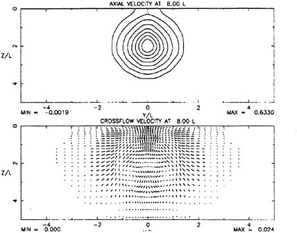
Figure 1. Mean flow in near-surface jet at x/d=8
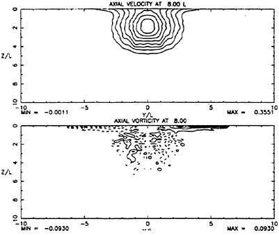
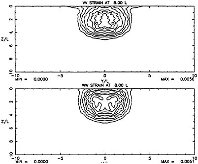
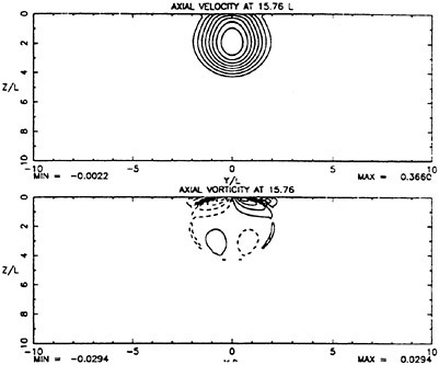
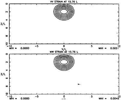
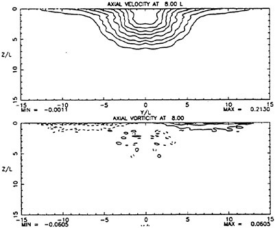
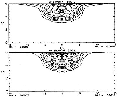
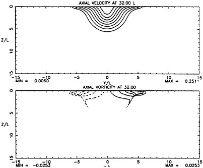
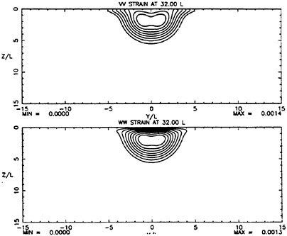
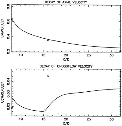
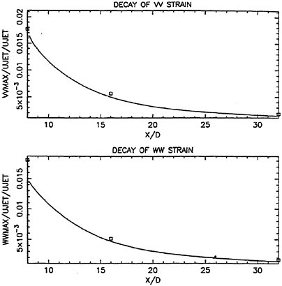
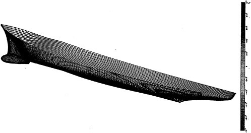
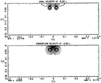
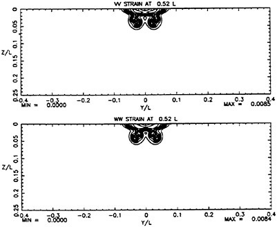
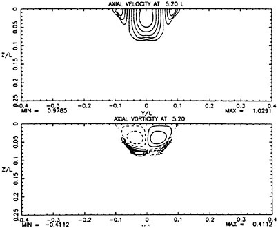
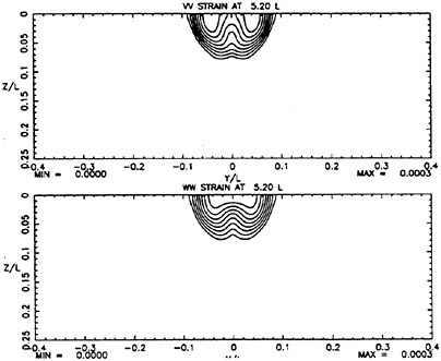
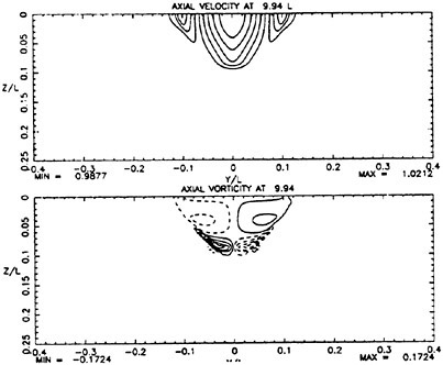
Figure 9a. Mean flow 10 L behind 5415 hull computed with algebraic stress model
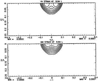
Figure 9b. Strain field 10 L behind 5415 hull computed with algebraic stress model
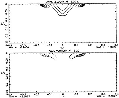
Figure 10a. Mean flow 5 L behind 5415 hull computed with algebraic stress model with free-surface interaction
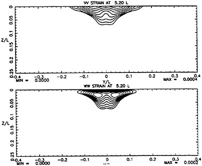
Figure 10b. Mean flow 5 L behind 5415 hull computed with algebraic stress model with free-surface interaction
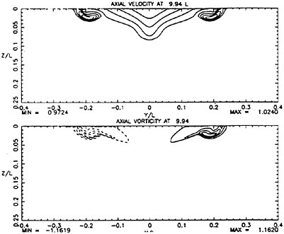
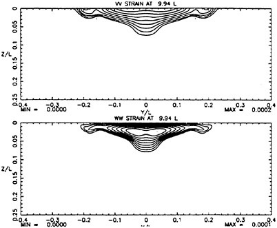
Applications of a Hybrid Boundary Element Method to the Analysis of Free-Surface Flow Around Lifting and Nonlifting Bodies
C.-Y.Hsin (National Taiwan Ocean University, Taiwan, China)
S.-K.Chou (United Ship Design and Development Center, Taiwan, China)
Abstract
The purpose of this paper is to present a hybrid boundary element method used to calculate the wave making resistance problems. In this method, the singularity strengths on a non-lifting body or a lifting body and the singularity strengths on the free surface are solve separately. For solving the body problems, Green’s identity formula is adopted, and a potential based boundary element method is used to solve the strengths of perturbation potentials (dipoles) distributed on the body surface by satisfying the solid body boundary condition. For lifting bodies, the Kutta condition has also to be imposed. For the free surface problem, a velocity based method is used to solve the strengths of sources distributed on the free surface. The influence to each other is then taken into account by considering the induced velocities as part of the inflow. The interactions between bodies and free surface are therefore solved by an iterative procedure. Numerical examples are shown in the paper, including nonlifting bodies, lifting bodies and bodies with multiple parts.
1 Introduction
Solving the wave resistance problems by a boundary element method, or a panel method, has been studied for more than thirty years. Hess and Smith [1] first presented a velocity based panel method to calculate the potential flow around an arbitrary three dimensional body, and Dawson [2] later modified Hess and Smith’s method to take the free surface effect into account. In Dawson’s method, sources are distributed on both the body surface and the free surface, and strengths of the sources distributed are determined by satisfying the solid body boundary condition on the body, and a linearized free surface boundary condition on the free surface.
For bodies with lifting effects traveling in a free surface, such as a surface piercing hydrofoil, dipoles or vortices have to be distributed on the body surface. Hess [3] modified his source only method with the inclusion of a constant strength vortex sheet distributed on the body surface, and the vortex strengths are determined by satisfying the Kutta condition. Xia [4] later applied this modified method to solve the wave making resistance problems of sailing boats. Xia’s method has kept the original structure of Dawson’s method, however, resulted in a complicated formulation due to the consideration of the lifting effect. Also, in order to satisfy the Kutta condition, an iterative procedure was needed for the solutions of nonlinear equations. Xu [5] and Maniar [6] used Havelock singularities to solve the free surface/lifting surface interaction problems, which the panels were only distributed on the body surface.
In the present paper, the authors use a different approach by solving the singularity strengths on the body surface and on the free surface separately. For solving the body problems, Green’s identity formula is adopted, and a potential based boundary element method is used to solve the strengths of perturbation potentials (dipoles) distributed on the body surface by satisfying the solid body boundary condition. For lifting bodies, a vortex sheet (wake) behind the body is introduced, and the Kutta condition has to be satisfied. For the free surface problem, a ve-
locity based method is used to solve the strengths of sources distributed on the free surface. The influence to each other is then taken into account by considering the induced velocities as part of the inflow. The interactions between bodies and free surface are therefore solved by an iterative procedure.
The concept of multi-zone boundary element method can also be applied to the presented method by appropriately dividing the body into several zones. That is, when solving the problem of free surface around a body with multiple parts, such as catamarans, trimarans, or the interaction between the ship hull and the propeller, similar iterations can also be used to compute the interactions between different parts.
2 Theory
Considering a body (a ship or a hydrofoil) traveling with a steady forward speed, U∞, in the presence of the free surface, we can assume that the total potential Φ to be the sum of the double-body potential, ![]() and the free surface perturbation potential,
and the free surface perturbation potential, ![]() as in Dawson’s [2] method.
as in Dawson’s [2] method.
(1)
If we assume ζ to be the wave elevation, then on the free surface z=ζ(x, y), the velocity potential needs to satisfy the Bernoulli’s equation
(2)
and the kinematics boundary condition
(3)
If l represents the derivatives along a streamline of the double-body potentials on the plane of z=0, we can then obtain the following equation from equations (1), (2), and (3):
(4)
The boundary condition on the wetted hydrofoil surface is the solid body boundary condition:
(5)
where Φn is the normal derivative of the total potential.
The above method has been widely applied to the wave resistance problems, in which sources are distributed on both the body surface and the free surface. Detailed derivation can been seen from [4] or other related documents. In the presented method, both source and dipole sheets are distributed on the body surface, and the Green’s identity method is used to solve the singularity strengths on the body. However, only sources are distributed on the free surface panels. The singularity strengths on the body and on the free surface are solved separately, and the influence to each other is taken into account by considering the induced velocities as part of the inflow velocities. Therefore,
-
When solving the body problem, the Green’s theorem is used,
(6)
where G is the Green function,
 . R(p; q) is the distance between points p and q, SB represents the body surface, and SW represents the body wake surface.
  is the perturbation potential, and can be explained as the dipole strength distributed on the body,
  is the source strength, and it is a known term from the solid body boundary condition.
(7)
where
 is the normal vector of the body,
  is the inflow velocity including the induced velocities on the body by the free surface panels
(8)
In equation (6),
 is the dipole strength in the body wake, and it is equivalent to the difference of the dipole strengths of panels on the upper and lower surfaces at the trailing edge. This kind of numerical Kutta condition has first been used by Morino [7], and later been applied to a propeller panel method by Kerwin et. al. [8]. It implies that the vortex strength at the trailing edge is zero, therefore, the pressures on the pressure side and on the suction side are equal at the trailing
-
edge. Since
 equals to the difference of the dipole strengths at the trailing edge panels, it can be coupled into the dipole term in equation (6). If we define the double body solution as the solution of zero Froude number, then the initial solution (first iteration) of the equations (6) and (7) are the solutions of double body problem. The term
  then represents the double body solutions,
  . In the following iterations, equations (6) and (7) are still solved, how ever, we will call the solutions as the solutions of the “body problem” since the free surface effect has been counted.
-
When solving the free surface problem, the derivative of the total potential in the streamline direction thus can be expressed as follows:
(9)
where
 can be calculated from equation (6), and
  where σ is the source strength on the free surface panel. Equation (4) thus can be solved.
In the above scheme, it needs an iterative procedure to include the interaction between the body and the free surface. A detail numerical procedure will be discussed in the next section.
3 Numerical Implementations
We have introduced the fundamental formulations needed in this method, and we will now describe the numerical implementations to carry out the theory. The step by step numerical procedur e is described as follows:
-
First, we solve the double-body problem by solving the discretized form of equation (6) with the boundary condition in equation (7). The discretized form of equation (6) can be seen form [8] or [9], and it represents a linear system to solve.
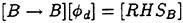
(10)
In equation (10), we define the left-hand-side matrix [B → B] as the “body to body” influence coefficients matrix. The right-hand-side matrix [RHSB] represents the influence of the source with the strength of and
 is equivalent to
  when solving
  the double body problem. We then cans obtain the solutions,
  by solving the above linear system.
 -
We then solve the free surface problem, that is, to solve equation (4).
-
 can be obtained by calculating the induced velocities of the body on the free surface panels,
 -
(Φ)l is calculated as in equation (9), note that
 is equivalent to
  in the first iteration,
 -
 and
and  can be obtained by using a finite difference method to
  .
.
-
-
A linear system thus can be set up from equation (4),
(11)
In equation (11), we define the left-hand-side matrix [F → F] as the “free surface to free surface” influence coefficients matrix. The source strengths of free surface panels, σf, thus can be calculated.
-
Calculate the induced velocities of the free surface panels to the body panels. The inflow velocity to the body is updated by including the free surface induced velocities as in equation (8), and the source strength distributed on the body surface is thus updated. The singularity strengths on the body can be solved again by solving equations (6), or, step 1. However, the double body solution,
 now is the solutions of the body problem.
 -
We can then repeat the step 2 by using the updated body problem solutions instead of double body solutions.
The whole procedure is repeated until solutions are converged.
In Dawson’s method, the matrix system can be written as follows:
(12)
where [B → B] is the “body to body” influence coefficients matrix, [F → B] is the “free surface
to body” influence coefficients matrix, [B → F] is the “body to free surface” influence coefficients matrix, and [F → F] is the “free surface to free surface” influence coefficients matrix, [σ] is the source strength distributed on both the body surface and free surface. The presented method actually decomposes the above matrix system into two systems (body problem and free surface problem), and [F → B] and [B → F] are solved through iterations. It is found that the left-hand-side matrices in solving both the body and free surface problems can be solved by an iterative matrix solver. The reason is that by solving the “body problem” and the “free surface problem” separately, the left-hand-side matrices become less ill-conditioned. Therefore, the computational time of solving the linear system is thus proportional to N2 rather than N3 (N is the number of elements in the matrix). Notice that the left-hand-side matrices are the same in every iteration, therefore, only the back substitutions are needed after the first iteration.
Because the interaction between the body and the free surface are carried out by the concept of “inflow” and solved iteratively, a body with multiple parts can also be computed by the presented method. The fundamental philosophy is still the same, however, there are two different ways to obtain the body solution. One way is to solve all the parts together just as described above. The other way is to obtain the solutions of each part, and the interaction between each other is carried out by the “inflow” concept. For example, when calculating the free surface around a catamaran, both approach can be used. However, the first approach may be easier. When investigating the interaction between the propeller and the ship hull, the latter approach may be more appropriate since the free surface effect is very small to the propeller.
4 Numerical Validations
In order to validate the presented method, we will demonstrate several numerical computations here, and these calculations include both the flow around non-lifting bodies and lifting bodies. The computational results will be used for the following purposes:
-
the comparison between the presented method and a source only method;
-
the comparison between the numerical results and the experimental data;
Figure 1: Comparison of the calculated wave pattern at Froude number 0.28 between the presented method and a source only, velocity based method.
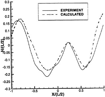
Figure 2: Comparison of the wave height at Froude number 0.28 between the computational results and the measured values (bow is at −1.0).
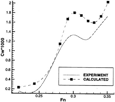
Figure 3: Comparison of the wave resistance coefficients, CW, between the computational results and the experimental data. CW is defined as ![]()
-
the ability to calculate the flow around bodies with multiple parts.
4.1 Non-Lifting Bodies in the Free Surface
As we mentioned in the previous sections, it is equivalent to compute a body in the zero angle of attack when calculating flow around non-lifting bodies. Therefore, the presented method can compute flow around non-lifting bodies without any modifications. Here we first test the presented method by computing the flow around a nonlifting body, and the case selected is the classical Series 60 ship hull with CB=0.6. We have calculated the flow around this ship hull at several different Froude numbers to obtain the wave profile and the wave resistance. The Froude number is defined as ![]() where L is the ship length. The computational results have been first compared with the computational results of a source-only, velocity based, Dawson’s type code [10]. Figure 1 shows the comparison of the calculated wave pattern at Froude number 0.28 between the presented method and this source only, velocity based method, and the comparison shows a good agree
where L is the ship length. The computational results have been first compared with the computational results of a source-only, velocity based, Dawson’s type code [10]. Figure 1 shows the comparison of the calculated wave pattern at Froude number 0.28 between the presented method and this source only, velocity based method, and the comparison shows a good agree
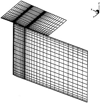
Figure 4: Arrangement of panels on the free surface and on the hydrofoil in the presented method.
ment between two methods. Note that both methods use exactly the same panel arrangements in the computations.
We then compare the computational results with the experimental data. The comparisons have been made between the computational results and the experimental data obtained by Kim and Jenkins [11]. Figure 2 shows the comparison of the wave height at Froude number 0.28 between the computational results and the measured values. In this figure, L is the ship length, and the ship bow and stern is located at x=−1.0 and x=+1.0 separately. Figure 3 then shows the comparison of the wave resistance coefficients, CW, between the computational results and the experimental data at different Froude numbers. Here, CW is defined as ![]() where S is the wetted surface area of the ship hull, and Vs is the ship speed. In figure 3, one can see that the computational results are reasonable but consistently higher than the experimental data. However, both values have the same trend as CW varying with the Froude numbers.
where S is the wetted surface area of the ship hull, and Vs is the ship speed. In figure 3, one can see that the computational results are reasonable but consistently higher than the experimental data. However, both values have the same trend as CW varying with the Froude numbers.
4.2 Lifting Bodies in the Free Surface
In order to validate the computations of
free surface around lifting bodies by using the presented method, the calculations of two surface piercing hydrofoils will be demonstrated here. These two hydrofoils are actually the same hydrofoil with different immersed length under water. The experiments have been conducted at David Taylor Model Basin, and forces on the hydrofoils have been measured at different Froude numbers and different yaw angles (angles of attack) [12]. The tested hydrofoil has a sectional geometry of NACA63A with 9% thickness to chord ratio. The chord length is 16.75 inches, and the span underwater are 57 inches for the “full span” case (the aspect ratio is 3.4), and 30 inches for the “half span” case (the aspect ratio is 1.9). In both cases, the forces on the hydrofoil have been measured when the hydrofoil traveling at 2 knots and 4 knots with several different yaw angles. We define the Froude number as ![]() here, where C is the hydrofoil chord length, then the above cases are equivalent to Froude numbers 0.5 and 1.0.
here, where C is the hydrofoil chord length, then the above cases are equivalent to Froude numbers 0.5 and 1.0.
In the presented method, the coordinate system is fixed on the body; therefore, the inflow directs with an angle of attack (yaw angle) when calculating the flow around a surface piercing hydrofoil with a yaw angle. As shown in figure 4, the panels on the free surface are aligned with the inflow direction, and the panels on the hydrofoil are discretized by using a cosine spacing in both the spanwise direction and the chordwise direction. This is for the purpose of having better numerical resolutions near the free surface and at leading edge and trailing edge. The panels on the free surface are discretized by a hyperbolic tangent spacing in the upstream and downstream of the hydrofoil, and aligned with the panels on the hydrofoil. The panels on the hydrofoil wake is discretized by a half-cosine spacing such that panels are finer near the hydrofoil trailing edge.
We first examine the convergence of computational results. Figure 5 shows the calculated circulation distributions by using different number of panels. In this figure, the nondimensional circulation, G, is defined as ![]() where Γ is the circulation strength, and R is the length of hydrofoil span. The solutions at both Froude numbers 0.0 and 0.5 are shown in figure 5, and the results of both cases are convergent. Note that the zero Froude number solutions are equivalent to the double-body solutions. Figure 6 shows the calculated wave height contour on the free surface for Froude number 0.5, and the yaw angle is 4 degrees. Although there is no experimental
where Γ is the circulation strength, and R is the length of hydrofoil span. The solutions at both Froude numbers 0.0 and 0.5 are shown in figure 5, and the results of both cases are convergent. Note that the zero Froude number solutions are equivalent to the double-body solutions. Figure 6 shows the calculated wave height contour on the free surface for Froude number 0.5, and the yaw angle is 4 degrees. Although there is no experimental
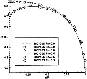
Figure 5: Calculated circulation distributions on the hydrofoil for Fn=0 and Fn=0.5 by using different number of panels. C represents number of panels in the chordwise direction, and S represents number of panels in the spanwise direction
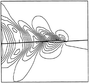
Figure 6: Wave height contour on the free surface of a “full span” hydrofoil calculated by the presented method, Fn=0.5, and the yaw angle is 4 degrees
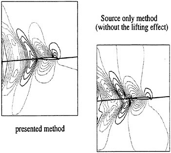
Figure 7: Comparison of the calculated wave pattern of the “full span” hydrofoil between the presented method and a source only, velocity based method. The Froude number is 0.5, and the yaw angle is 4 degrees.
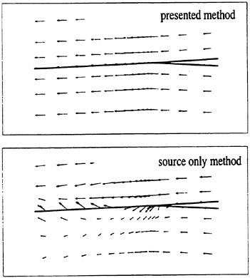
Figure 8: Comparison of the calculated velocities near the hydrofoil trailing edge of the “full span” hydrofoil between the presented method and a source only, velocity based method. The Froude number is 0.5, and the yaw angle is 4 degrees.
data available for the c|omparison, the wave pattern looks reasonable. We then investigate the lifting effect and the Kutta condition. Figure 7 shows the computational wave patterns using the presented method, and the presented method without the lifting effect. To implement the latter one, we simply force the dipole strength in the hydrofoil wake to be zero, and this is equivalent to “turn off” the Kutta condition. By doing this, the computational results have been found to be the same as those from a source only, velocity based method. From figure 7, the difference between two calculations is obvious. It is more interesting to investigate the detail flow near the trailing edge of these two computations, and figure 8 shows the velocities calculated by these two different codes. Apparently, imposing the Kutta condition makes the flow smooth near the trailing edge as one has expected.
We will then compare the calculated forces and measured forces on the hydrofoil. In the presented method, the forces are calculated by integrating the pressures on the foil surface. Figures 9 and 10 show the comparisons of the lift coefficients between the computational results and experimental data at two different Froude numbers for the “full span” case (aspect ratio=3.4). For both Froude numbers, computational results fail to predict the lift coefficients at 8 degrees of yaw angles, however, the comparisons of the computational results and the experimental data are good at smaller yaw angles. Figures 11 and 12 show the comparisons of the lift coefficients between the computational results and experimental data at two different Froude numbers for the “half span” case (aspect ratio=1.9). For these cases, the computational results agree well with the experimental data at 8 degrees of yaw angles, and the comparison is especially good for Froude number 1.0. For all the cases, the computational lift coefficients are linear with respect to the angle of attack. However, this is not true for the experimental data. Therefore, more comparisons should be done for conclusions. After all, the above comparisons show that the presented method can predict the forces on a surface piercing hydrofoil reasonably accurate.
4.3 A Body with Multiple Parts
In this section, we have shown numerical results of both the lifting and nonlifting bodies, and finally, we will demonstrate numerical results of a body with multiple parts. As described earlier, there
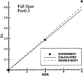
Figure 9: Comparison of the computational lift coefficients and experimental data at Froude numbers 0.5 for the “full span” case.
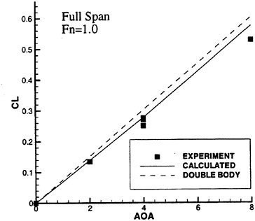
Figure 10: Comparison of the computational lift coefficients and experimental data at Froude numbers 1.0 for the “full span” case.
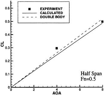
Figure 11: Comparison of the computational lift coefficients and experimental data at Froude numbers 0.5 for the “half span” case.
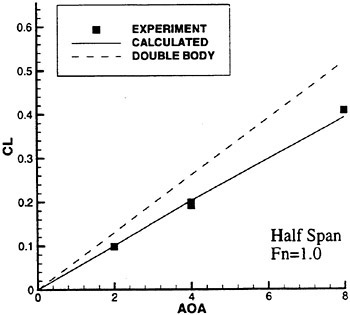
Figure 12: Comparison of the computational lift coefficients and experimental data at Froude numbers 1.0 for the “half span” case.
are two ways to solve the multiple parts problem in the presented method. One is to solve all the parts together, and the other one is to solve one by one. Here we will demonstrate the calculation of the interaction between two surface piercing hydrofoils. Both hydrofoils have the same configurations: NACA66 sections with 10% thickness to chord ratio, aspect ratios of 5.9, and the hydrofoils travel with an equivalent Froude number 0.5. Figure 13 shows the wave generated by two surface piercing hydrofoils, and the distance between hydrofoils is half the chord length. Figure 13 shows the wave generated by two surface piercing hydrofoils, and the distance between hydrofoils is half the chord length. Figure 14 shows a similar result, but the distance between hydrofoils is twice the chord length. From these two figures, one can see the wave pattern generated by a system of two hydrofoils, also one can see the interference of two wave systems. We know that the interference effect between these two hydrofoils will result in an asymmetrical velocity field to these two hydrofoils, and generate a suction side force to each other. Figure 15 shows the calculated side force coefficients with respect to different distance between two hydrofoils, and the side force coefficient is defined as ![]() . The side force coefficient is below 2% when two hydrofoils are appart one chord length, and drops to 0.0005 for twice the chord length.
. The side force coefficient is below 2% when two hydrofoils are appart one chord length, and drops to 0.0005 for twice the chord length.
5 Conclusions
In this paper, the authors have described a boundary element method to solve the problem of a surface piercing hydrofoil. This method uses a potential based method to solve the body problem, and a velocity based method to solve the free surface problem. The interactions between two are then considered by an iterative procedure.
The advantage of the presented method is that it is easy to implement the Kutta condition, and when the lifting effect is considered, the formulation used is not more complicated than the original Dawson’s source only method. This method is also easy to be extended to the solutions of a body with multiple parts. To solve the body problem and the free surface problem separately by using different boundary element methods, the resulting matrices for both problems can be solved by an iterative matrix solver. Therefore, solutions time of the matrices is more efficient.
Computational results for free surface flow
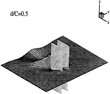
Figure 13: Wave generated by two surface piercing hydrofoils, and the distance between these two hydrofoils is half the hydrofoil chord length.
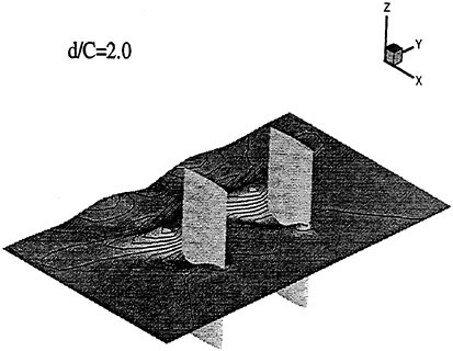
Figure 14: Wave generated by two surface piercing hydrofoils, and the distance between these two hydrofoils is twice the hydrofoil chord length.
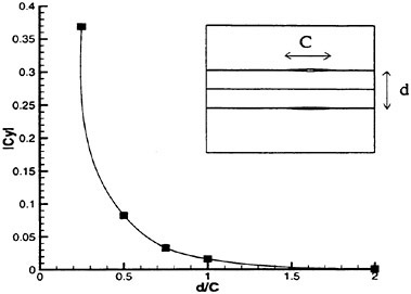
Figure 15: Side force coefficients on the hydrofoil calculated by the presented method at different distance between two hydrofoils
around nonlifting bodies, lifting bodies and bodies with multiple parts have been demonstrated. The comparison between the presented method and a source only method shows that results from the presented method is very close to the latter method for nonlifting bodies. The effect of the Kutta condition is also shown by this comparison. The comparison between the numerical results and the experimental data have been shown, and reasonable agreements between the numerical results and the experimental data can always be obtained. The ability to calculate the flow around bodies with multiple parts by the presented method is also demonstrated in the paper, and analysis of flow around a catamaran, or a SWATH should be able to be done by the presented method.
For the future work, in addition to the fine tune of the method, it is authors’ intention to extend the presented method to the solutions of the time domain, unsteady inflow problems.
References
[1] J.L.Hess and A.M.O.Smith. Calculation of nonlifting potential flow about arbitrary three dimensional bodies. Journal of Ship Research, vol 8(no 2), September 1964.
[2] C.W.Dawson. A practical computer method for solving ship wave problems. In Proceedings of the Second International Conference on Numerical Ship Hydrodynamics, 1977.
[3] J.L.Hess. Calculation of Potential flow About Arbitrary Three-Dimensional Lifting Bodies. Technical Report MDC J5679–01, McDonnell Douglas, October 1972.
[4] Fei Xia. Calculation of Lifting Potential Flow with a Free Surface. Technical Report 2912–2, SSPA, April 1986.
[5] Hongbo Xu. Potential flow solution for a yawed surface-piercing plate. Journal of Fluid Mechanics, vol 226, 1991.
[6] H.Maniar, J.N.Newman, and H.Xu. Free-surface effects on a yawed surface-piercing plate. In Proceedings of the Eighteenth Symposium on Naval Hydrodynamics, Ann Arbor, Michigan, August 1990.
[7] Luigi Morino and Ching-Chiang Kuo. Subsonic potential aerodynamic for complex configurations: a general theory. AIAA Journal, vol 12(no 2):pp. 191–197, February 1974.
[8] J.E.Kerwin, S.A.Kinnas, J-T Lee, and W-Z Shih. A surface panel method for the hydrodynamic analysis of ducted propellers. Trans. SNAME, 95, 1987.
[9] Ching-Yeh Hsin, Justin E.Kerwin, and Spyros A.Kinnas. A panel method for the analysis of the flow around highly skewed propellers. In Proceedings of the Propellers/Shafting ’91 Symposium, SNAME, Virginia Beach, VA, September 1991.
[10] C.-Y.Lu and S.-K.Chou. A computational method for calculating ship wave resistance. In Proceedings of CFD Workshop, Tokyo, Japan, 1994.
[11] Y.H.Kim and D.Jenkins. Trim and Sinkage Effects on Wave Resistance with Series 60, CB=0.6. Technical Report DTRC/SPD-1013–011, David Taylor Research Center, 1981.
[12] W.E.Beaver. PACT Surface Piercing Foil Experiments—Experiment Description and Force Data. Technical Report DTRC/SHD-1358–01, David Taylor Research Center, April 1991.
DISCUSSION
U.Bulgarelli
Istituto Nazionale per Studi ed Esperienze di Architettura Navale, Italy
In the case of nonlifting body, when you use the so-called Morino’s condition, do you use some dynamical condition for the wake?
AUTHORS’ REPLY
The Morino’s Kutta condition is applied to the lifting bodies, and this condition has no effect for a non-lifting body since the dipole strength on the wake equals zero. For the lifting bodies, the dipole strength on the wake is determined by the Morino’s Kutta condition, and the wake geometry is given. No other dynamical condition is imposed. References [7], [8], and [9] have more detailed descriptions of the Morino’s Kutta condition.
DISCUSSION
H.Söding
Technical University Hamburg-Harburg, Germany
The authors combine a direct (source-dipole) method for lift generating bodies with an indirect (source only) method for the free surface. To me this appears better, in view of accurate lift force predictions, than what Zou and I did in our work presented at the ONR Symp. 1994, where we used for the body an indirect method with sources along the body surface and a vortex lattice along the body centerplane. Whether the solution is attained iteratively and separately for free surface and body singularities, or in one step for the combined system, appears to me as a minor detail.
Regarding Fig. 3 (where a factor of 103 is missing), I added Cw values (dots) which I condensed from various model experiments summarized by Kajitani (A wandering in some resistance components and flow, Ship Techn. Res. 34/3, 1987, 105–131). According to this source, the author’s wave resistance coefficients are correct up to Fn=0.3, and a little too small for Fn>0.3. The figure shows that experimental inaccuracy and the subdivision of the measured total resistance into wave and viscous contributions amounts to errors which may be larger than computational inaccuracy. This seems remarkable especially in view of the fact that only the linearized and not fully correct (see Jensen, Söding and Mi, ONR Symposium 1986) free surface condition of Dawson was used.
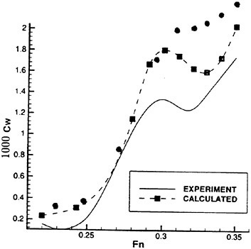
Regarding the Kutta condition, most authors use the difference of the potential between pressure and suction side in the center of the last panel for the dipole strength in the wake. My experience is that it is better to extrapolate the potential from the panel center to the trailing edge, using also the last but one panel of equal height. This may eliminate the need to use very narrow panels near the trailing edge where the flow is quite smooth.
The practically interesting point in partly immersed foils is ventilation on the suction side, occurring in rudders, hydrofoils and their struts. This requires a nonlinear free surface condition to be applied along a nearly vertical free surface. It appears worthwhile if the authors tried to extend their method to such cases.
AUTHORS’ REPLY
Thanks for Professor Söding’s comments. For the comparison of the CW, the authors replot the Figure 3 with the experimental data Professor Söding has used (marked as Kajitani), and it shows in the figure below.
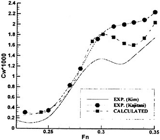
The experimental data used in the paper are from reference [11], and the computational results presented in this paper do agree better with Kajitani’s experimental data especially for the Fn less than 0.3. Since there may be different approaches for obtaining CW from the model tests, it is hard to draw a conclusion here. In any case, the authors will make more comparisons between the computational results and the experimental data to validate the presented method.
Regarding the Kutta condition, the authors’ experience is that the extrapolation technique Professor Söding suggested usually does not have an encouraging outcome for a foil section with a high camber ratio. However, a linear dipole distribution, or even higher order distribution, on the panel does provide a more accurate solution near the trailing edge. A paper written by Kinnas and Hsin (Kinnas and Hsin, “On the Local Error of a Low-order Boundary Element Method at the Trailing Edge of a Hydrofoil and Its Effect on the Global Solution,” Computers and Fluids Journal, January, 1994, pp. 63–75) presents this finding. For complicated three-dimensional geometries such as marine propellers, a pressure Kutta condition may even be needed besides the Morino’s Kutta condition (References [8] and [9]).
The United Ship Design and Development Center (where one of the authors, Dr. Chou, is working) has developed a source only free surface code satisfying the non-linear free surface boundary condition, and the authors do have the intention to implement the scheme used in that code into the presented method in the future.
DISCUSSION
R.Yeung
University of California at Berkeley, USA
If I may say so, the title of the paper is a misnomer. Normally, a “hybrid” method is used to refer to a combination of two or more computational methodologies. What is discussed here is essentially an integral-equation method that utilizes a kind of “block structuring” algorithm to make it easier for data assembly and solution speed.
On the point about the usage of the “Morino” condition as a Kutta condition, this was utilized extensively since a couple of works in the 2nd International Numerical Ship Hydrodynamics Conference (1977). Similar techniques were used in airfoil/hydrofoil flows (e.g., Yeung and Banger, 1977) to treat the Kutta condition. I do find the applications here quite interesting.
AUTHORS’ REPLY
Thanks for Professor Yeung’s comments. The reason we used the word “hybrid” is that we have used the different formulations (potential based and velocity based boundary element methods) to treat the body and the free surface separately. In some sense, it is not only a “block structuring” algorithm. However, we will try to figure out a better name for the presented method in the future work.
Regarding Morino’s Kutta condition, Professor Morino used it in his 1974 paper (Reference 7), and this condition was then extensively utilized for different problems. One of the applications is for the analysis of the flow around marine propellers. Many papers written by Professor Kerwin and his colleagues at MIT have discussed the effect of this condition in solving the propeller problems (for example, References 8 and 9). The authors do find that this condition can be applied to solving the surface piercing hydrofoil problems as well. More discussion about the Morino’s Kutta condition can be seen in the reply to Professor Söding.
Super Green Functions
X.-B.Chen (Bureau Veritas, France)
F.Noblesse (Naval Surface Warfare Center, Carderock Division, USA)
ABSTRACT
Free-surface potential flows generated by arbitrary distributions of singularities, e.g. sources and dipoles distributed over curved hull-panels or waterline-segments, are considered. Such flows are called super Green functions because of their similarities and differences with classical Green functions, which correspond to point sources instead of distributions of singularities. Fourier representations of super Green functions are given for generic dispersive media, and applied to the specific case of time-harmonic free-surface flows with forward speed. These representations of super Green functions are simple, well suited for accurate and efficient numerical evaluation (both in the far field and in the near field) and provide useful decompositions of near-field dispersive waves into wave components and nonoscillatory local components (negligible in the far field) given by single and double Fourier integrals, respectively. The ship-motion Green function, which includes major built-in advantages (proper far-field wavy behavior, radiation condition) can therefore be used with the same ease as Rankine singularities.
INTRODUCTION: GREEN FUNCTIONS AND SUPER GREEN FUNCTIONS
In potential flows, a Green function ![]() defines the velocity potential of the flow created at a point
defines the velocity potential of the flow created at a point ![]() by a source of unit strength located at a point
by a source of unit strength located at a point ![]() . The Green function for an unbounded incompressible fluid is
. The Green function for an unbounded incompressible fluid is
where r is the distance between the field point ![]() and the singular point
and the singular point ![]() . In free-surface hydrodynamics, Green functions can be expressed as
. In free-surface hydrodynamics, Green functions can be expressed as
(1)
where GF accounts for free-surface effects and GS is defined in terms of simple singularities. For instance, in the case of time-harmonic free-surface flows with forward speed in deep water, which is of primary interest in this study, the simple-singularity component GS is given by
where r′ is the distance between ![]() and the mirror image of
and the mirror image of ![]() with respect to the mean free-surface plane z=0. The free-surface component GF is defined by a double Fourier integral.
with respect to the mean free-surface plane z=0. The free-surface component GF is defined by a double Fourier integral.
For time-harmonic ship waves in infinite water depth, the free-surface component GF is given by the Fourier superposition of elementary waves
(2a)
where ![]() is the wavenumber and
is the wavenumber and
(2b)
Furthermore, D is the dispersion function
(3a)
and sign(Df)=sign(∂D/∂f) is given by
(3b)
The dispersion function (3a) is associated with the classical free-surface boundary condition
linearized about the uniform stream opposing the forward speed of the ship. The nondimensional frequency f, the Froude number F, and the Brard number τ are defined as
where ω is the encounter frequency of the regular ambient waves exciting the ship motions, L and U are the ship length and forward speed, and g is the acceleration of gravity.
Two basic difficulties restrict the practical utility of free-surface Green functions. One major difficulty is that the double Fourier integral representation (2a) of free-surface effects is singular and cannot be evaluated accurately (except in very few relatively simple cases like time-harmonic flows without forward speed, for which the near-field behavior of GF can be determined analytically [1]) in the critically-important limit (X, Y, Z) → 0. Another difficulty is that Green functions are not directly useful (except for idealized cases involving flows about spheres) for practical applications, which require flows generated by distributions of singularities (sources and dipoles) over hull-panels and waterline-segments instead of point singularities.
Indeed, practical calculations involve distributions of singularities of the form
(4)
where P stands for a hull-panel or a waterline-segment near a point1![]() and σ and
and σ and ![]() are source and dipole densities, respectively. A function (4) associated with a distribution of singularities is called a super Green function because of its similarities and differences with usual Green functions, associated with point singularities. In the usual approach in which G and ∇G are evaluated using (2) and subsequently integrated over a panel or a segment as in (4), the super Green functions
are source and dipole densities, respectively. A function (4) associated with a distribution of singularities is called a super Green function because of its similarities and differences with usual Green functions, associated with point singularities. In the usual approach in which G and ∇G are evaluated using (2) and subsequently integrated over a panel or a segment as in (4), the super Green functions ![]() associated with free-surface flows cannot be evaluated accurately for field points near a waterline-segment or a hull-panel at the free surface.
associated with free-surface flows cannot be evaluated accurately for field points near a waterline-segment or a hull-panel at the free surface.
However, the super Green functions ![]() of main interest in free-surface hydrodynamics (and their derivatives) can be evaluated in a remarkably simple way using Kochin’s formulation [2] and the Fourier representation of free-surface effects developed here. Within the Fourier-Kochin formulation, the free-surface-effect component
of main interest in free-surface hydrodynamics (and their derivatives) can be evaluated in a remarkably simple way using Kochin’s formulation [2] and the Fourier representation of free-surface effects developed here. Within the Fourier-Kochin formulation, the free-surface-effect component
(5)
of the super Green function
is defined by substituting (2) into (5) and performing the space integration over the hull-panel or the waterline-segment before the Fourier integration. Thus, the free-surface component ![]() is given by the double Fourier integral representation
is given by the double Fourier integral representation
(6a)
where
(6b)
and S is the spectrum function defined as
(7a)
(7b)
The integral representations (2) and (6) of the free-surface components GF and ![]() of the related Green function G and super Green function
of the related Green function G and super Green function ![]() show that GF is a special case of
show that GF is a special case of ![]() corresponding to
corresponding to
An important property of the spectrum function (7) associated with a distribution of singularities is
As a result, the super Green function ![]() defined by (6) is finite in the limit (X, Y, Z) → 0, whereas GF is singular in this limit. Furthermore, space integration over a hull-panel or a waterline-segment is incomparably simpler in (7a), where the elementary wave-function (7b) is infinitely differentiable, than in (5) which involves functions GF and ∇GF singular for (X, Y, Z)=0. Thus, the Fourier-Kochin representation of super Green functions given by (6) and (7) effectively circumvents the two previously-noted basic difficulties restricting the utility of the classical approach based on (2) and (5). In this approach, influence coefficients (which are an important class of super Green functions) in fact cannot be evaluated with accuracy for field (control) points in the vicinity of a distribution of singularities over a waterline-segment or a hull-panel at the free surface, as already noted. However, the Fourier-Kochin representation (6) and (7) makes it possible to evaluate influence coefficients in all cases, including the most difficult and important2 case involving a waterline-segment or a hull-panel at the free surface.
defined by (6) is finite in the limit (X, Y, Z) → 0, whereas GF is singular in this limit. Furthermore, space integration over a hull-panel or a waterline-segment is incomparably simpler in (7a), where the elementary wave-function (7b) is infinitely differentiable, than in (5) which involves functions GF and ∇GF singular for (X, Y, Z)=0. Thus, the Fourier-Kochin representation of super Green functions given by (6) and (7) effectively circumvents the two previously-noted basic difficulties restricting the utility of the classical approach based on (2) and (5). In this approach, influence coefficients (which are an important class of super Green functions) in fact cannot be evaluated with accuracy for field (control) points in the vicinity of a distribution of singularities over a waterline-segment or a hull-panel at the free surface, as already noted. However, the Fourier-Kochin representation (6) and (7) makes it possible to evaluate influence coefficients in all cases, including the most difficult and important2 case involving a waterline-segment or a hull-panel at the free surface.
The space integration (7) in the Fourier-Kochin representation of super Green functions is a trivial
task, as was already noted. However, the Fourier integration (6a) is a nontrivial issue. This critical issue is considered in [3–5] and here for generic dispersion and spectrum functions D and S, i.e. for arbitrary singularity distributions in generic dispersive media. Indeed, although super Green functions are defined above for time-harmonic ship waves in deep water, a broad class of dispersive waves (including water waves in finite water depth and internal waves in a density-stratified fluid) are defined by the generic Fourier representation (6). This Fourier representation of dispersive waves is now considered.
Specifically, the super Green ![]() function defined by the Fourier representation
function defined by the Fourier representation
(8)
is considered for generic dispersion and amplitude functions D and A. We define polar coordinates
(9)
We may assume that the amplitude function A(α, β) in (8) vanishes as k → ∞ and does not oscillate rapidly, as follows from (7).
GENERIC DISPERSIVE WAVES: FAR-FIELD WAVES
It is shown in [3] that the double Fourier integral (8) can be expressed in the basic form
(10)
where ![]() is the double Fourier integral
is the double Fourier integral
(11)
obtained by formally setting ε=0 in (8), and ![]() is given by the single Fourier integrals
is given by the single Fourier integrals
(12)
along the dispersion curves defined by the dispersion relation3D=0. In (12) and elsewhere, ∑D=0 means summation over all the dispersion curves, ds is the differential element of arc length of a dispersion curve, and ![]() with Dα=∂D/∂α and Dβ=∂D/∂β.
with Dα=∂D/∂α and Dβ=∂D/∂β.
(11) indicates that the functions ![]() and g2(α, β)≡A/D are Fourier transforms. The theory
and g2(α, β)≡A/D are Fourier transforms. The theory
|
3 |
The dispersion relation usually defines several dispersion curves, although a single dispersion curve may exist in some cases; e.g. wave diffraction-radiation without forward speed |
of Fourier transforms [6] indicates that the behavior of the function ![]() in the limit H → ∞ is determined by the singularities of the Fourier transform g2(α, β), i.e. by the dispersion relation D=0. Thus, the far-field waves contained in (11) are determined by the dispersion curves defined by the dispersion relation. Specifically, we have
in the limit H → ∞ is determined by the singularities of the Fourier transform g2(α, β), i.e. by the dispersion relation D=0. Thus, the far-field waves contained in (11) are determined by the dispersion curves defined by the dispersion relation. Specifically, we have
(13)
where ![]() is given by the single Fourier integrals [5]
is given by the single Fourier integrals [5]
(14)
along the dispersion curves. Here, Θ is defined as
(15)
where erf is the usual error function, k* is a reference wavenumber, and σ is a positive real number. The reference wavenumber k* may be taken equal to the local value of the wavenumber k at the dispersion curve. Other reference wavenumbers may be used; e.g., for free-surface flows, k*=f2 and k*=1/F2 are proper choices for time-harmonic flows without forward speed and steady flows [7].
By using (13) in (10) we obtain
(16)
where
(17)
is defined by (12) and (14) as
(18)
The terms sign(Df) and Θ stem from the components ![]() and
and ![]() respectively, in the basic representation (10) of the super Green function
respectively, in the basic representation (10) of the super Green function ![]() . The sign function sign(Df), associated with the limit ε → +0 in (8), ensures satisfaction of the radiation condition, and the function Θ accounts for the far-field waves contained in the double Fourier integral
. The sign function sign(Df), associated with the limit ε → +0 in (8), ensures satisfaction of the radiation condition, and the function Θ accounts for the far-field waves contained in the double Fourier integral ![]() .
.
In the far-field limit H → ∞, (15) yields
(19)
The Fourier representation of generic far-field dispersive waves defined by (18) and (19), given in [3], is a special case of the representation defined by (18) and (15). Specifically, (19) corresponds to a far-field approximation of (15) as was just shown. The function (19) is independent of the parameter σ in (15)
and indeed corresponds to the limit σ=0 of (15). The Fourier integral (18) can be further approximated using the method of stationary phase. The stationary-phase approximation of (18) yields simple relations, given in [8], between the dispersion curves D=0 and important aspects (wavelengths, directions of wave propagation, phase and group velocities, and cusp angles) of the corresponding farfield waves.
GENERIC DISPERSIVE WAVES: NEAR-FIELD REPRESENTATIONS
In the near field, the generic super Green function (8) can be expressed as the sum of a wave component ![]() and a local component
and a local component ![]() :
:
(20)
where ![]() is defined as
is defined as ![]() . The constant σ in expression (15) for the function Θ in (18) may be chosen so that the local component
. The constant σ in expression (15) for the function Θ in (18) may be chosen so that the local component ![]() decays without oscillations, i.e. so that the wave component
decays without oscillations, i.e. so that the wave component ![]() fully accounts for the waves included in
fully accounts for the waves included in ![]() in the near field (as well as in the far field where
in the near field (as well as in the far field where ![]() is negligible and
is negligible and ![]() ). Thus, both the wave component
). Thus, both the wave component ![]() and the local component
and the local component ![]() in (20) involve σ, although the sum is
in (20) involve σ, although the sum is ![]() of course independent of σ, like the far-field approximation of
of course independent of σ, like the far-field approximation of ![]() given by (18) and (19).
given by (18) and (19).
The near-field decomposition (20) into wave and local components is nonunique. The function Θ in expression (18) for the wave component is taken as (19) in [4], where a Fourier representation of the corresponding local component ![]() is given. Here, the function Θ in (18) is taken as (15), obtained in [5]. Expression (19), given in [3] and used in [4], is a particular case of (15), which involves σ; indeed, (19) corresponds to a far-field approximation or the limit σ → 0 of (15) as already noted.
is given. Here, the function Θ in (18) is taken as (15), obtained in [5]. Expression (19), given in [3] and used in [4], is a particular case of (15), which involves σ; indeed, (19) corresponds to a far-field approximation or the limit σ → 0 of (15) as already noted.
The integrand of the double Fourier integral representation of ![]() given in [4] is continuous everywhere but varies rapidly across a dispersion curve. Here, the more general representation (15) of the function Θ is used, as already noted, and a remarkably simple Fourier representation of the corresponding local component
given in [4] is continuous everywhere but varies rapidly across a dispersion curve. Here, the more general representation (15) of the function Θ is used, as already noted, and a remarkably simple Fourier representation of the corresponding local component ![]() is given. The near-field representation of
is given. The near-field representation of ![]() given here is mathematically exact (whereas the representation of
given here is mathematically exact (whereas the representation of ![]() given in [4] involves numerical approximations) and is well suited for accurate and efficient numerical evaluation. In particular, the integrand of the double Fourier integral in the expression for the local component
given in [4] involves numerical approximations) and is well suited for accurate and efficient numerical evaluation. In particular, the integrand of the double Fourier integral in the expression for the local component ![]() given further on is continuous everywhere and varies slowly across a dispersion curve.
given further on is continuous everywhere and varies slowly across a dispersion curve.
Expressions (10) and (17) show that the local component ![]() is given by
is given by
(21)
This basic representation of the local component ![]() is ill suited for numerical calculations because the double Fourier integral (11) cannot be evaluated acccurately. Practical near-field Fourier representations, suited for accurate evaluation, of the local component
is ill suited for numerical calculations because the double Fourier integral (11) cannot be evaluated acccurately. Practical near-field Fourier representations, suited for accurate evaluation, of the local component ![]() associated with the generic Fourier representation (8), (20), (18), (15) of dispersive waves are given below for two common cases. These two cases correspond to dispersion functions that define two basic classes of dispersion curves, called simple open dispersion curves and simple closed dispersion curves. These classes of dispersion curves, and the corresponding near-field representations of super Green functions, are examined below. A more general Fourier representation for dispersion curves of arbitrary shape is given in [9].
associated with the generic Fourier representation (8), (20), (18), (15) of dispersive waves are given below for two common cases. These two cases correspond to dispersion functions that define two basic classes of dispersion curves, called simple open dispersion curves and simple closed dispersion curves. These classes of dispersion curves, and the corresponding near-field representations of super Green functions, are examined below. A more general Fourier representation for dispersion curves of arbitrary shape is given in [9].
GENERIC DISPERSIVE WAVES : SIMPLE OPEN DISPERSION CURVES
The case of a dispersion relation D=0 that yields a single dispersion curve defined by a single-valued function α=αd(β) with −∞<β<∞ is considered first. Thus, it is now assumed that every constant-β line intersects the dispersion curve only once. Such a dispersion curve is called a simple open dispersion curve of type A. Expression (12) yields
where the relation ds/∥∇D∥=dβ/|Dα| was used and α=αd(β). In the vicinity of the dispersion curve α=αd(β) the amplitude and dispersion functions can be approximated as A~Ad and ![]() where Ad and
where Ad and ![]() are the values of A and Dα at the dispersion curve. By using these approximations in (11) we can express
are the values of A and Dα at the dispersion curve. By using these approximations in (11) we can express ![]() . The component
. The component ![]() is given by
is given by
Here, the subscript or superscript d was deleted, and k* and σ are the reference wavenumber and the parameter defined in (15). By using the foregoing expressions for ![]() and in (17)
and in (17) ![]() we obtain
we obtain
with
(22a)
The relation dβ/|Dα|=ds/∥∇D∥ may be used to express ![]() in the form (18).
in the form (18).
In the more general case a dispersion function that defines several simple open dispersion curves of type A, defined by single-valued functions α=αj(β) with −∞<β<∞, ![]() is defined by (18) with Θ given by (22a). The local component is
is defined by (18) with Θ given by (22a). The local component is ![]() given by
given by

(22b)
where Aj and ![]() represent the values of A and Dα at the jth dispersion curve α=αj(β), and the localizing function
represent the values of A and Dα at the jth dispersion curve α=αj(β), and the localizing function ![]() is defined as
is defined as
(22c)
Here ![]() is the reference wavenumber attached to the jth dispersion curve. The integrand of (22b) is finite at a dispersion curve. Specifically, we have
is the reference wavenumber attached to the jth dispersion curve. The integrand of (22b) is finite at a dispersion curve. Specifically, we have
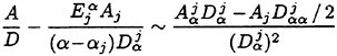
(23)
as α → αj, where ![]() and
and ![]() are the values of Αα and Dαα at the jth dispersion curve.
are the values of Αα and Dαα at the jth dispersion curve.
The near-field representation (22) of dispersive waves may be used for a dispersion function that yields simple open dispersion curves, of type A, defined by single-valued functions α=αj(β) with −∞<β<∞. This generic Fourier representation is applied to steady ship waves in [7] and to time-harmonic ship waves in this study. An analogous Fourier representation is given in [9] for a dispersion function that yields one or more simple open dispersion curves, of type B, defined by single-valued functions β=βj(α) with −∞<α<∞.
At a point where Dα or Dβ vanishes, as occurs if the functions αj(β) or βj(α) defining the dispersion curves are not single valued, the function given by (23) or the similar function given in [9] for simple open dispersion curves of type Β are singular, respectively. However, the near-field representation (22) for simple open dispersion curves of type A and the analogous representation for simple open dispersion curves of type Β given in [9] can be generalized to the case of arbitrary dispersion curves, that cannot be defined by single-valued functions αj(β) or βj(α). The more general near-field Fourier representation of dispersive waves, required for time-harmonic ship waves in the narrow band ![]() is given in [9].
is given in [9].
GENERIC DISPERSIVE WAVES: SIMPLE CLOSED DISPERSION CURVE
The case of a dispersion function that defines a closed dispersion curve surrounding a point (α0,β0) in the Fourier plane is now considered. Polar Fourier variables centered at (α0, β0) are defined:
(24a)
(24b)
It is assumed here that the dispersion curve can be defined by a single-valued function ρ=ρd(γ) with −π≤/≤π. Such a dispersion curve is called a simple closed dispersion curve. (24) and (9) yield
(25)
By using the relation ds/∥∇D∥=ρddγ/|Dρ| and (25) in (12) we obtain
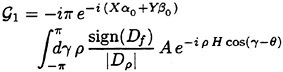
where ρ=ρd(γ). Similarly, (11) becomes
In the vicinity of the dispersion curve ρ=ρd(γ) we have ρ ~ ρd, A ~ Ad and ![]() where Ad and
where Ad and ![]() stand for the values of A and Dρ at the dispersion curve. By using these approximations we can express
stand for the values of A and Dρ at the dispersion curve. By using these approximations we can express ![]() in the form
in the form ![]() . The component
. The component ![]() is given by
is given by
where the subscript and superscript d were deleted, k* and σ are the reference wavenumber and the parameter defined in (15), and Θ is given by
(26a)
By substituting the foregoing expressions for ![]() and
and ![]() into (17) we obtain
into (17) we obtain
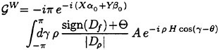
The relation ρdγ/|Dρ|=ds/∥∇D∥ and (25) show that this integral representation of the wave component ![]() is identical to (18).
is identical to (18).
The local component ![]() is given by
is given by
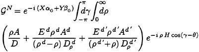
(26b)
Here, ρd and ρd′ are defined as
(26c)
Ad, ![]() and Ad′,
and Ad′, ![]() stand for the values of A and Dρ at the points (ρd, γ) and (ρd′, γ+π):
stand for the values of A and Dρ at the points (ρd, γ) and (ρd′, γ+π):
(26d)
and similarly for ![]() and
and ![]() . Finally, the localizing functions Ed and Ed′ are given by
. Finally, the localizing functions Ed and Ed′ are given by
(26e)
(26f)
The integrand of (26b) is easily shown to be continuous at the dispersion curve.
The near-field representation (26) of dispersive waves may be used for a dispersion function that yields a simple closed dispersion curve, surrounding a point (α0, β0) of the Fourier plane, defined by a single-valued function ρ=ρd(γ), with ρ and γ given by (24). This generic Fourier representation is applied to diffraction-radiation of water waves without forward speed in [7] and to time-harmonic ship waves (in the regime τ<1/4) in this study.
APPLICATIONS TO TIME-HARMONIC SHIP WAVES
The foregoing Fourier representations of super Green functions in generic dispersive media are now applied to a specific class of dispersive waves. This class of dispersive waves is characterized by the dispersion function (3a), which corresponds to time-harmonic free-surface flows with forward speed in deep water. Two interesting special cases of time-harmonic flows with forward speed are time-harmonic flows without forward speed (F=0) and steady flows (f=0), for which the dispersion function (3a) respectively becomes
These classes of flows correspond to the complementary special cases F=0 with f≠0 and f=0 with F≠0 of the limit τ=f F=0. For time-harmonic flows without forward speed, the dispersion relation D=0 defines a single simple closed dispersion curve (the circle k=f2 centered at the origin of the Fourier plane) and the representation (26) may be applied. For steady flows, we have two simple dispersion curves of type A, which are symmetric with respect to both α=0 and β=0, and the representation (22) may be applied. The Fourier representations of super Green functions for wave diffraction-radiation without forward speed and steady ship waves are given in [7]. The case τ≠0 is considered here.
TIME-HARMONIC SHIP WAVES: DISPERSION CURVES
The dispersion function (3a) shows that the dispersion curves D=0 are symmetric with respect to β=0 and, in the region β≥0, are given by
(27)
In the Fourier upper half plane, the expression ds/∥∇D∥=dα/|Dβ| for the differential element of arc length ds of a dispersion curve and (3a) yield
(28)
This relation is used further on. The dispersion relation D=0 defines two or three dispersion curves if τ is larger or smaller than 1/4.
If τ<1/4, the three dispersion curves intersect the axis β=0 at four values of α, which are denoted ![]() and
and ![]() and are given by
and are given by
(29)
The three dispersion curves are found in the regions
(30a)
If τ=1/4, (29) yield
and the dispersion curves in the regions ![]() and
and ![]() are connected. If τ>1/4, the roots
are connected. If τ>1/4, the roots ![]() and
and ![]() are complex and we only have two dispersion curves, located in the regions
are complex and we only have two dispersion curves, located in the regions
(30b)
The inner roots ![]() and the outer roots
and the outer roots ![]() satisfy the inequalities
satisfy the inequalities
(31)
The inequalities (31) show that the sign function sign(Df) defined by (3b) is equal to −1 for the dispersion curve in the region ![]() and to 1 for the other dispersion curves. The dispersion curves defined by (27), (29) and (30) are depicted for several values of τ in Fig. 1, where the Fourier plane is scaled with respect to f/F.
and to 1 for the other dispersion curves. The dispersion curves defined by (27), (29) and (30) are depicted for several values of τ in Fig. 1, where the Fourier plane is scaled with respect to f/F.
In the limit τ=0, (29) yield ![]() and
and ![]() . More generally, we have
. More generally, we have
Thus, the dispersion curves in the outer regions ![]() and
and ![]() correspond to values of the wavenumber k that are greater than 1/F2 (approximately), whereas we have k≈f2 for the dispersion curve in the inner region
correspond to values of the wavenumber k that are greater than 1/F2 (approximately), whereas we have k≈f2 for the dispersion curve in the inner region ![]() . The ratio of the wavenumbers ki and ko associated with the inner and outer dispersion curves, given by ki/ko≈τ2, is very small if τ is small, say if τ≤0.2. Thus, scaling of the Fourier coordinates α and β with respect to f2 and 1/F2 is proper in this regime. The upper and lower parts of Fig. 2 respectively depict the inner and outer dispersion curves for several values of τ in the frequency-scaled and speed-scaled Fourier planes (α, β)/f2 and F2(α, β). Finally, (29) yield
. The ratio of the wavenumbers ki and ko associated with the inner and outer dispersion curves, given by ki/ko≈τ2, is very small if τ is small, say if τ≤0.2. Thus, scaling of the Fourier coordinates α and β with respect to f2 and 1/F2 is proper in this regime. The upper and lower parts of Fig. 2 respectively depict the inner and outer dispersion curves for several values of τ in the frequency-scaled and speed-scaled Fourier planes (α, β)/f2 and F2(α, β). Finally, (29) yield
Thus, scaling of the Fourier coordinates with respect to f/F is proper for large values of τ.
TIME-HARMONIC SHIP WAVES : COMPONENT WAVE SYSTEMS
The dispersion curves in the regions (30) yield distinct contributions to the wave component ![]() . For τ<1/4,
. For τ<1/4, ![]() can be expressed in the form
can be expressed in the form
(32a)
The components ![]() and respectively
and respectively ![]() correspond to the dispersion curves in the inner region
correspond to the dispersion curves in the inner region ![]() and the outer regions
and the outer regions ![]() and
and ![]() . The component
. The component ![]() represents a system of ring-like waves, called ring waves here. The components
represents a system of ring-like waves, called ring waves here. The components ![]() and
and ![]() represent two systems of V-like waves contained within wedges and called outer V waves and inner V waves, respectively. Curves of constant phase (e.g. crest lines) corresponding to the ring waves (thick solid lines), the outer V waves (dashed lines), and the inner V waves (thin solid lines) are depicted in the upper part of Fig. 3 for τ=0.24. In the limit τ=0, the components
represent two systems of V-like waves contained within wedges and called outer V waves and inner V waves, respectively. Curves of constant phase (e.g. crest lines) corresponding to the ring waves (thick solid lines), the outer V waves (dashed lines), and the inner V waves (thin solid lines) are depicted in the upper part of Fig. 3 for τ=0.24. In the limit τ=0, the components ![]() and
and ![]() respectively correspond to the time-harmonic ring waves (limit F=0) and the steady ship waves (limit f=0) considered in [7].
respectively correspond to the time-harmonic ring waves (limit F=0) and the steady ship waves (limit f=0) considered in [7].
For τ>1/4, ![]() can be expressed as
can be expressed as
(32b)
where ![]() and
and ![]() are associated with the dispersion curves in the regions
are associated with the dispersion curves in the regions ![]() and
and ![]() respectively. The component
respectively. The component ![]() represents a system of inner V waves qualitatively similar to the inner V waves in (32a). The component
represents a system of inner V waves qualitatively similar to the inner V waves in (32a). The component ![]() represents fan-like waves and incomplete ring waves. These waves are also contained within a wedge, and are called ring-fan waves. The system of ring-fan waves can be further divided into two systems of waves: a system of inner fan waves and a system of partial ring waves and outer fan waves, which correspond to the portions α≤−f/F and
represents fan-like waves and incomplete ring waves. These waves are also contained within a wedge, and are called ring-fan waves. The system of ring-fan waves can be further divided into two systems of waves: a system of inner fan waves and a system of partial ring waves and outer fan waves, which correspond to the portions α≤−f/F and ![]() of the dispersion curve
of the dispersion curve ![]() . Constant-phase curves corresponding to the partial ring waves and the outer fan waves (thick solid lines), the inner fan waves (dashed lines), and the inner V waves (thin solid lines) are depicted in the lower part of Fig. 3 for τ=0.26.
. Constant-phase curves corresponding to the partial ring waves and the outer fan waves (thick solid lines), the inner fan waves (dashed lines), and the inner V waves (thin solid lines) are depicted in the lower part of Fig. 3 for τ=0.26.
The components ![]() and
and ![]() in the decompositions (32) of the wave component
in the decompositions (32) of the wave component ![]() are considered in [10] using the Fourier representation of
are considered in [10] using the Fourier representation of ![]() given by (18) and (19). As noted previously, this representation of
given by (18) and (19). As noted previously, this representation of ![]() is a far-field approximation of the representation given by (18) and (15), which is used here. The analysis of far-field time-harmonic ship waves given in [10] is completed in this study using the near-field Fourier representation of
is a far-field approximation of the representation given by (18) and (15), which is used here. The analysis of far-field time-harmonic ship waves given in [10] is completed in this study using the near-field Fourier representation of ![]() given above4. Thus, the near-field analysis of the super Green function
given above4. Thus, the near-field analysis of the super Green function ![]() defined by (3), (6) and (7), corresponding to an arbitrary distribution of pulsating singularities in translation, expounded below extends the far-field analysis considered in [10].
defined by (3), (6) and (7), corresponding to an arbitrary distribution of pulsating singularities in translation, expounded below extends the far-field analysis considered in [10].
TIME-HARMONIC SHIP WAVES: INNER V WAVES
The inner V wave component ![]() exists for all values of τ and corresponds to the simple open dispersion curve of type A in the region
exists for all values of τ and corresponds to the simple open dispersion curve of type A in the region ![]() where
where ![]() is given by (29). Inner V waves are represented in terms of coordinates scaled with respect to the reference wavenumber
is given by (29). Inner V waves are represented in terms of coordinates scaled with respect to the reference wavenumber ![]()
(33a)
The dispersion relation yields ![]() along the dispersion curve
along the dispersion curve ![]() . The upper half of this dispersion curve is defined by
. The upper half of this dispersion curve is defined by
The function Γ is defined as
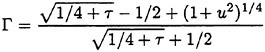
(33b)
with 0≤u<∞. (29) and the relations ![]() and
and ![]() were used. The parameter u is roughly equal to the scaled Fourier variable
were used. The parameter u is roughly equal to the scaled Fourier variable ![]() .
.
We have sign(Df)=−1 and sign(Dα)=1 along the dispersion curve ![]() . By using these relations, (22a), (28), and the foregoing parametric representation of the dispersion curve in (18) we obtain
. By using these relations, (22a), (28), and the foregoing parametric representation of the dispersion curve in (18) we obtain
(33c)
where ![]() is the wave integral
is the wave integral
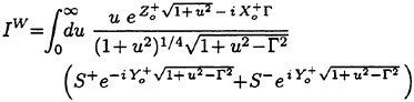
(33d)
Here S± stand for the values of S(α, β) at ![]() and
and ![]() . We have
. We have
Thus, the integrand of (33d) is continuous for u≥0.
TIME-HARMONIC SHIP WAVES: OUTER V WAVES
The outer V wave component ![]() which only exists if r<1/4, corresponds to the simple open dispersion curve of type A in the region
which only exists if r<1/4, corresponds to the simple open dispersion curve of type A in the region ![]() where
where ![]() is given by (29). Outer V waves are represented in terms of coordinates scaled with respect to the reference wavenumber
is given by (29). Outer V waves are represented in terms of coordinates scaled with respect to the reference wavenumber ![]()
(34a)
The dispersion relation yields ![]() along the dispersion curve
along the dispersion curve ![]() . The upper half of this dispersion curve is defined by
. The upper half of this dispersion curve is defined by
The function Γ is defined as
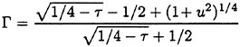
(34b)
with 0≤u<∞. (29) and the relations ![]() and
and ![]() were used. The parameter u is roughly equal to the scaled Fourier variable
were used. The parameter u is roughly equal to the scaled Fourier variable ![]() .
.
We have sign(Df)=1 and sign(Dα)=−1 along the dispersion curve ![]() . By using these relations, (22a), (28), and the foregoing parametric representation of the dispersion curve in (18) we obtain
. By using these relations, (22a), (28), and the foregoing parametric representation of the dispersion curve in (18) we obtain
(34c)
where ![]() is the wave integral
is the wave integral
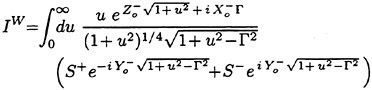
(34d)
Here S± stand for the values of S(α, β) at ![]() and
and ![]() . We have
. We have
Thus, the integrand of (34d) is continuous for u≥0.
In the limit τ=0, the V wave ![]() component given by (32a) and (33)–(34) is identical to the wave component for steady flows given in [7]. Thus, although the components
component given by (32a) and (33)–(34) is identical to the wave component for steady flows given in [7]. Thus, although the components ![]() and
and ![]() contain real and imaginary parts, the sum
contain real and imaginary parts, the sum ![]() is real if τ=0.
is real if τ=0.
TIME-HARMONIC SHIP WAVES: RING-FAN WAVES
The ring-fan wave component ![]() which only exists if τ>1/4, corresponds to the dispersion curve in the region
which only exists if τ>1/4, corresponds to the dispersion curve in the region ![]() where
where ![]() is given by (29). The case
is given by (29). The case ![]() for which every constant-β line intersects the dispersion curve
for which every constant-β line intersects the dispersion curve ![]() only once and (22) may be used, is now considered. Ring-fan waves are represented in terms of coordinates scaled with respect to the reference wavenumber
only once and (22) may be used, is now considered. Ring-fan waves are represented in terms of coordinates scaled with respect to the reference wavenumber ![]()
(35a)
The dispersion relation yields ![]() along the dispersion curve
along the dispersion curve ![]() . The upper half of this dispersion curve is defined by
. The upper half of this dispersion curve is defined by
The function Γ is defined as
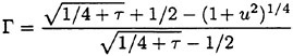
(35b)
with 0≤u<∞. (29) and the relations ![]() and
and ![]() were used. The parameter u is roughly equal to the scaled Fourier variable
were used. The parameter u is roughly equal to the scaled Fourier variable ![]() .
.
We have sign(Df)=1 and sign(Dα)=−1 along the dispersion curve ![]() . By using these relations, (22a), (28), and the foregoing parametric representation of the dispersion curve in (18) we obtain
. By using these relations, (22a), (28), and the foregoing parametric representation of the dispersion curve in (18) we obtain
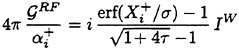
(35c)
where ![]() is the wave integral
is the wave integral
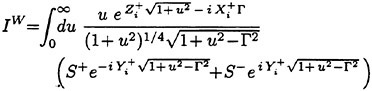
(35d)
Here S± stand for the values of S(α, β) at ![]() and
and ![]() . We have
. We have
Thus, the integrand of (35d) is continuous for u≥0.
TIME-HARMONIC SHIP WAVES: RING WAVES
The ring wave component ![]() which only exists if τ<1/4, is associated with the simple closed dispersion curve in the inner region
which only exists if τ<1/4, is associated with the simple closed dispersion curve in the inner region ![]() where
where ![]() are given by (29). Ring waves are represented in terms of coordinates scaled with respect to the reference wavenumber k*=f2:
are given by (29). Ring waves are represented in terms of coordinates scaled with respect to the reference wavenumber k*=f2:
(36a)
The center point (α0, β0) in (24) is taken at the origin of the Fourier plane. The upper half of the dispersion curve is defined by
where the frequency-scaled wavenumber Γ=k/f2 is given by
(36b)
with 0≤γ≤π. In the limit τ → 0, Γ → 1 and the inner dispersion curve becomes a circle of radius k=f2 centered at the origin of the Fourier plane [7].
We have sign(Df)=1 and sign(Dk)=−1 along the inner dispersion curve. By using these relations, the relation ds/∥∇D∥=kdγ/|Dk|, (3a), (36b), and (26a) in (18) we obtain
(36c)
where IW(Xω, Υω, Ζω) is the wave integral
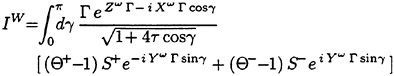
(36d)
Here S± are the values of S(a, β) at β=±f2 Γ sinγ and α=f2 Γ cosγ, and Θ± are given by
(36e)
The integrand of (36d) is continuous for 0≤γ≤π. In the limit τ=0, the ring wave component (36) is identical to the wave component for diffraction-radiation without forward speed given in [7].
TIME-HARMONIC SHIP WAVES: LOCAL FLOW DISTURBANCE
The local component ![]() in (20) is now considered for the two cases
in (20) is now considered for the two cases ![]() and τ≤1/4.
and τ≤1/4.
Case 
If ![]() we have two dispersion curves, located in the regions (30b). The contributions of these dispersion curves to the wave component
we have two dispersion curves, located in the regions (30b). The contributions of these dispersion curves to the wave component ![]() yield the ring-fan waves
yield the ring-fan waves ![]() and the inner V waves
and the inner V waves ![]() —in accordance with (32b)—defined by (35) and (33), respectively, which follow from the generic representation (22) for simple open dispersion curves of type A. Expression (22b) yields
—in accordance with (32b)—defined by (35) and (33), respectively, which follow from the generic representation (22) for simple open dispersion curves of type A. Expression (22b) yields
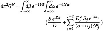
(37)
where Δα=−Dα. Here, j=1 and j=2 correspond to the dispersion curves in the regions ![]() and
and ![]() respectively. These dispersion curves are defined by α=αj(β) where αj are the two real roots of the dispersion relation D=0. (3a) yields
respectively. These dispersion curves are defined by α=αj(β) where αj are the two real roots of the dispersion relation D=0. (3a) yields
(38)
Sj stands for the value of S(α, β) at (αj, β), and ![]() is defined by (22c) where the reference wavenumber
is defined by (22c) where the reference wavenumber ![]() is given by
is given by ![]() and
and ![]() .
.
Case τ<1/4
If τ<1/4 we have three dispersion curves, located in the regions (30a). As is indicated in (32a), the contributions of these dispersion curves to the wave component ![]() yield the ring waves
yield the ring waves ![]() associated with the closed dispersion curve in the inner region
associated with the closed dispersion curve in the inner region ![]() and the V waves
and the V waves ![]()
associated with the open dispersion curves in the outer regions ![]() and
and ![]() . The ring waves are defined by (36) and the V waves by (34) and (33). In the limit τ=0, the ring waves
. The ring waves are defined by (36) and the V waves by (34) and (33). In the limit τ=0, the ring waves ![]() and the V waves
and the V waves ![]() are identical to the wave component for diffraction-radiation without forward speed (F=0) and the wave component for steady flows (f=0), respectively [7]. Thus, the particular cases F=0 and f=0 correspond to the limit F → 0 with f≠0 and the limit f → 0 with F≠0, which are distinct complementary limits included in the limit τ → 0. The local component
are identical to the wave component for diffraction-radiation without forward speed (F=0) and the wave component for steady flows (f=0), respectively [7]. Thus, the particular cases F=0 and f=0 correspond to the limit F → 0 with f≠0 and the limit f → 0 with F≠0, which are distinct complementary limits included in the limit τ → 0. The local component ![]() can be expressed as
can be expressed as
(39)
where the components ![]() and
and ![]() stem from the contributions of the inner region k=O(f2) and the outer region k=O(1/F2) of the Fourier plane, respectively. Thus, the generic free-surface potential
stem from the contributions of the inner region k=O(f2) and the outer region k=O(1/F2) of the Fourier plane, respectively. Thus, the generic free-surface potential ![]() can be expressed as
can be expressed as
(40)
The inner-outer decomposition (39) of the local component ![]() is now considered.
is now considered.
It is useful to define the blending functions
These functions satisfy the conditions ![]() and
and ![]() . Furthermore, if the positive real constant C is chosen sufficiently small, say if C≤1/5, we have
. Furthermore, if the positive real constant C is chosen sufficiently small, say if C≤1/5, we have ![]() and
and ![]() for
for ![]() and
and ![]() and
and ![]() for
for ![]() . Expressions (29) yield
. Expressions (29) yield
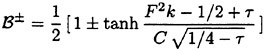
(41)
If τ≪1 we have ![]() which readily yields
which readily yields ![]() and
and ![]() . Thus, we have
. Thus, we have ![]() and
and ![]() in the inner region k≤f2, and
in the inner region k≤f2, and ![]() and
and ![]() in the outer region k≥1/F2 as already noted. The spectrum function S may be expressed as
in the outer region k≥1/F2 as already noted. The spectrum function S may be expressed as ![]() . The components
. The components ![]() and
and ![]() in (39) represent the contributions of the components
in (39) represent the contributions of the components ![]() and
and ![]() .
.
The component ![]() is defined by (22b) as
is defined by (22b) as
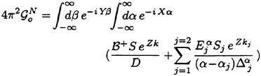
(42)
where Δα=−Dα. Also, the relation ![]() at the dispersion curves in the outer regions was used. Here, j=1 and j=2 correspond to the dispersion curves in the outer regions
at the dispersion curves in the outer regions was used. Here, j=1 and j=2 correspond to the dispersion curves in the outer regions ![]() and
and ![]() respectively. These dispersion curves, associated with the wave components
respectively. These dispersion curves, associated with the wave components ![]() and are
and are ![]() defined by α=αj(β) where αj are the two outer roots of the dispersion relation D=0. (3a) shows that
defined by α=αj(β) where αj are the two outer roots of the dispersion relation D=0. (3a) shows that ![]() is given by (38). Furthermore, Sj stands for the value of S at (αj, β), and
is given by (38). Furthermore, Sj stands for the value of S at (αj, β), and ![]() is defined by (22c) where the reference wavenumber
is defined by (22c) where the reference wavenumber ![]() is given by
is given by ![]() and
and ![]() .
.
The component ![]() is defined by (26b) as
is defined by (26b) as
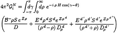
(43)
Here, the relation ![]() at the inner dispersion curve ρ=ρd(γ) was used, and ρ≡k and γ are the polar Fourier variables (24) centered at the origin of the Fourier plane. (3a) yields
at the inner dispersion curve ρ=ρd(γ) was used, and ρ≡k and γ are the polar Fourier variables (24) centered at the origin of the Fourier plane. (3a) yields
Furthermore, the notation defined in (26) was used. Thus, ρd and ρd′ are given by (26c), Sd, ![]() and Sd′,
and Sd′, ![]() stand for the values of S and Dρ at the points (ρd, γ) and (ρd′, γ+π), as in (26d), and Ed and Ed′ are given by (26e) and (26f) with k*=f2.
stand for the values of S and Dρ at the points (ρd, γ) and (ρd′, γ+π), as in (26d), and Ed and Ed′ are given by (26e) and (26f) with k*=f2.
TIME-HARMONIC SHIP WAVES: ILLUSTRATIVE APPLICATIONS
The foregoing Fourier representations of the super Green function for time-harmonic free-surface flows with forward speed are now applied to the practical task of evaluating influence coefficients, which are main building blocks within typical numerical solution procedures based on boundary-integral flow-representations. An example related to a low-order panel method is considered.
Specifically, we consider a uniform surface distribution of sources with density m over a flat rectangular panel Hp of length 2hp and depth dp contained in a vertical plane making an angle θp with the x axis. This source panel is centered at the point (xp, yp, zp≤0) and is defined by x=xp+u cosθp, y=yp+u sinθp and z=zp+v with −hp≤u≤hp and −dp≤v≤0. The velocity potential of ![]() the flow due to this distribution of sources is given by
the flow due to this distribution of sources is given by ![]() where the potentials
where the potentials ![]() and
and ![]() correspond to the simple-singularity and free-surface
correspond to the simple-singularity and free-surface
components GS and GF in expression (1) for the Green function.
Only the influence coefficient CF associated with the free-surface-effect component ![]() is considered here. Specifically, we consider the influence coefficient CF defined via a Galerkin integration5 of the free-surface potential
is considered here. Specifically, we consider the influence coefficient CF defined via a Galerkin integration5 of the free-surface potential ![]() over a flat rectangular panel Hq of length 2hq and depth dq contained in a vertical plane making an angle θq with the x axis. The influenced panel Hq is centered at the point (ξq, ηq, ζq≤0) and is defined by ξ=ξq+u cosθq, η=ηq+u sinθq and ζ=ζq+v with −hq≤u≤hq and −dq≤v≤0.
over a flat rectangular panel Hq of length 2hq and depth dq contained in a vertical plane making an angle θq with the x axis. The influenced panel Hq is centered at the point (ξq, ηq, ζq≤0) and is defined by ξ=ξq+u cosθq, η=ηq+u sinθq and ζ=ζq+v with −hq≤u≤hq and −dq≤v≤0.
The free-surface influence coefficient CF can be expressed as
(44a)
where ![]() is defined by (6a) with
is defined by (6a) with
(44b)
(44c)
(44d)
(44c) and (44d) yield S=1 for k=0 and S → 0 as k → ∞. More precisely, we have S=O(1/k4) as k → ∞, except along the rays γ=θp±π/2 and γ=θq±π/2 where we have S=O(1/k3). In the special case when θq=θρ we have S=O(1/k2) as k → ∞ along the rays γ=θp±π/2.
The free-surface influence coefficient ![]() normalized with respect to the source strength m and the areas of the source panel Hp and of the influenced panel Hq, is evaluated for panels Hp and Hq of sizes hp=0.025=hq and dp=0.015=dq in Figs 4 and 5. Furthermore, the orientations of Hp and Hq with respect to the x axis are chosen as θp=π/4 and θq=−π/4, and both panels are located at the free surface. Thus, we have Ζ=0 in (44b) and (6a).
normalized with respect to the source strength m and the areas of the source panel Hp and of the influenced panel Hq, is evaluated for panels Hp and Hq of sizes hp=0.025=hq and dp=0.015=dq in Figs 4 and 5. Furthermore, the orientations of Hp and Hq with respect to the x axis are chosen as θp=π/4 and θq=−π/4, and both panels are located at the free surface. Thus, we have Ζ=0 in (44b) and (6a).
Figs 4a,b,c respectively depict the inner-V wave component ![]() the ring-fan wave component
the ring-fan wave component ![]() and the local component
and the local component ![]() of the free-surface influence coefficient
of the free-surface influence coefficient
for τ=0.3 (F=0.25 and f=1.2). Similarly, Figs 5a,b,c respectively depict the V wave component ![]() the ring wave component
the ring wave component
![]() and the local component
and the local component ![]() of the free-surface influence coefficient
of the free-surface influence coefficient
for τ=0.2 (F=0.15 and f=4/3). Each of the six figures 4a,b,c and 5a,b,c is divided into a top half and a bottom half, which respectively correspond to the real and imaginary parts of the functions depicted in Figs 4a,b,c and 5a,b,c. The parameter σ in the Fourier representations of the wave and local components is taken equal to 0.2 for the calculations presented in Figs 4a,b,c and 5a,b,c.
Fig. 4a depicts the inner-V wave component ![]() in the region
in the region
where ![]() and
and ![]() are the coordinates defined by (33a). The top part and
are the coordinates defined by (33a). The top part and ![]() the bottom part
the bottom part ![]() show the real and imaginary parts of
show the real and imaginary parts of ![]() respectively, as noted already. Fig. 5a depicts the V wave component
respectively, as noted already. Fig. 5a depicts the V wave component ![]() in the region
in the region
where ![]() and
and ![]() are the coordinates defined by (34a). Fig. 4b depicts the ring-fan wave component
are the coordinates defined by (34a). Fig. 4b depicts the ring-fan wave component ![]() in the region
in the region
where ![]() and
and ![]() are the coordinates defined by (35a). Fig. 5b depicts the ring wave component
are the coordinates defined by (35a). Fig. 5b depicts the ring wave component ![]() in the region
in the region
where Χω and Υω are the coordinates defined by (36a). Finally, Figs 4c and 5c depict the local component ![]() in the region
in the region
These two figures show that the local component ![]() decays rapidly and without oscillations.
decays rapidly and without oscillations.
SUMMARY AND CONCLUSIONS
The functions D and A in expression (8) for the super Green function ![]() stand for generic dispersion and amplitude functions. Thus, the Fourier representation (8) is representative of a broad class of dispersive waves, including water waves in finite uniform water depth and internal waves in a density-stratified fluid, generated by an arbitrary distribution of singularities (e.g. localized polynomial distributions of sources and/or dipoles over curved hull-panels or waterline-segments, or global distributions over a whole ship hull).
stand for generic dispersion and amplitude functions. Thus, the Fourier representation (8) is representative of a broad class of dispersive waves, including water waves in finite uniform water depth and internal waves in a density-stratified fluid, generated by an arbitrary distribution of singularities (e.g. localized polynomial distributions of sources and/or dipoles over curved hull-panels or waterline-segments, or global distributions over a whole ship hull).
The near-field representation (20) expresses the generic super Green function ![]() as the sum of a wave component
as the sum of a wave component ![]() which is dominant in the far field, and a nonoscillatory local component
which is dominant in the far field, and a nonoscillatory local component ![]() negligible in the far field but significant in the near field. The
negligible in the far field but significant in the near field. The
wave component ![]() defined by (18) and (15), is expressed in terms of single Fourier integrals along the curves, called dispersion curves, defined by the dispersion relation D=0. The local
defined by (18) and (15), is expressed in terms of single Fourier integrals along the curves, called dispersion curves, defined by the dispersion relation D=0. The local ![]() component is given by a double Fourier integral.
component is given by a double Fourier integral.
Expressions for the wave component ![]() and the local component
and the local component ![]() are given for simple open dispersion curves, said to be of type A, defined by single-valued functions α=αj(β) with −∞<β< ∞ and for simple closed dispersion curves. The generality6 and simplicity of these near-field representations of the generic super Green function (8), given by (18) and (22) for simple open dispersion curves of type A and by (18) and (26) for simple closed dispersion curves, are remarkable properties of the near-field representations (18), (22) and (26), which are notable also in that they are suited for accurate numerical evaluation.
are given for simple open dispersion curves, said to be of type A, defined by single-valued functions α=αj(β) with −∞<β< ∞ and for simple closed dispersion curves. The generality6 and simplicity of these near-field representations of the generic super Green function (8), given by (18) and (22) for simple open dispersion curves of type A and by (18) and (26) for simple closed dispersion curves, are remarkable properties of the near-field representations (18), (22) and (26), which are notable also in that they are suited for accurate numerical evaluation.
The generic near-field Fourier representations for simple open dispersion curves of type A and for simple closed dispersion curves are applied to the super Green function (6) for time-harmonic ship waves, where the spectrum function S is associated with an arbitrary distribution of singularities as indicated in (7). Two cases are considered:
-
the regime
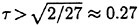 for which the dispersion function (3a) yields two simple open dispersion curves of type A, and
 -
the regime τ<1/4 for which we have a simple closed dispersion curve and two simple open dispersion curves of type A.
The near-field Fourier representations of the super Green function (6) for time-harmonic ship-waves in the regimes ![]() and τ<1/4 are given by the decompositions (32) into wave and local components. The corresponding Fourier representations of the inner and outer V wave components
and τ<1/4 are given by the decompositions (32) into wave and local components. The corresponding Fourier representations of the inner and outer V wave components ![]() and
and ![]() the ring-fan wave component
the ring-fan wave component ![]() the ring wave component
the ring wave component ![]() and the local component
and the local component ![]() provide simple expressions suited for accurate numerical evaluation of time-harmonic ship waves generated by arbitrary distributions of singularities for all values of τ except the narrow band
provide simple expressions suited for accurate numerical evaluation of time-harmonic ship waves generated by arbitrary distributions of singularities for all values of τ except the narrow band ![]() . Corresponding Fourier representations of the generic super Green function (6) for the particular cases of steady flows (f=0) and time-harmonic flows without forward speed (F=0) are given in [7].
. Corresponding Fourier representations of the generic super Green function (6) for the particular cases of steady flows (f=0) and time-harmonic flows without forward speed (F=0) are given in [7].
In the narrow band ![]() the dispersion function (3a) defines two open dispersion curves. One of these open dispersion curves is a simple curve of type A. However, some constant-β lines intersect the other dispersion curve at three
the dispersion function (3a) defines two open dispersion curves. One of these open dispersion curves is a simple curve of type A. However, some constant-β lines intersect the other dispersion curve at three
|
6 |
the functions D and A in these Fourier representations stand for generic dispersion and amplitude functions |
points. Thus, the generic Fourier representation for simple open dispersion curves of type A cannot be used in this case, for which a more general representation for dispersion curves of arbitrary shape is required. This general Fourier representation of the generic super Green function (8) is given in [9].
An important property of the decompositions, given by (20) and (32), into wave and local components is that they yield a corresponding decomposition of hydrodynamic loads into added-mass and wave-damping components, which are defined by single Fourier integrals.
The Fourier representation of time-harmonic free-surface flows with forward speed generated by arbitrary distributions of singularities given here makes it possible to use free-surface Green functions, which offer important built-in advantages (proper far-field behavior, radiation condition), with the same ease as Rankine singularities. E.g.:
-
Free-surface Green functions can be employed in a calculation method based on linearization about the double-body flow. Indeed, free-surface Green functions can be distributed over a small region of the mean free surface in the vicinity of a ship since the Kelvin free-surface boundary condition is nearly exact at a small distance from a ship.
-
The boundary-integral representation of time-harmonic free-surface potential flows with forward speed given in [11] and the Fourier representation of the related super Green function given here can also be used to couple a near-field calculation method, e.g. a potential-flow method based on Rankine singularities or a viscous-flow method, and an outer linear free-surface potential-flow representation.
Indeed, the Fourier representation of super Green functions for time-harmonic ship waves given here and the related boundary-integral representation given in [11] provide a new mathematical basis for solving the ship-motion problem in the frequency domain. An important property of the mathematical developments given here and in [11] is that they can be extended to the more general and difficult case of wave diffraction-radiation with forward speed in finite uniform water depth.
ACKNOWLEDGMENTS
The work of the first author was supported in part by a research grant from the DGA. We wish to thank Dr. Iwashita for providing results of his numerical evaluations of the ship-motion Green function, which were useful to check our calculations7.
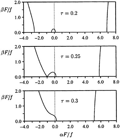
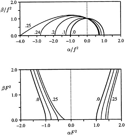
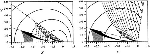
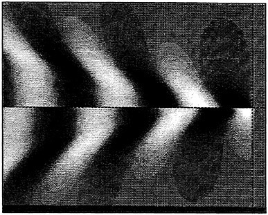
Fig. 4a Wave component ![]() for τ=0.3 in the region
for τ=0.3 in the region ![]() and
and ![]()
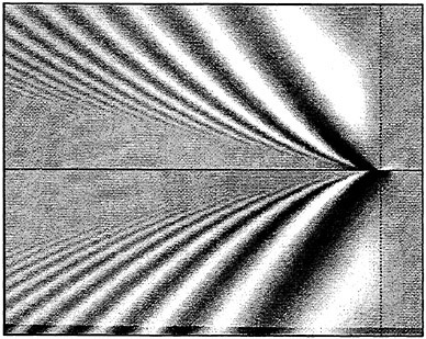
Fig. 4b Wave ![]() component for τ=0.3 in the region
component for τ=0.3 in the region ![]() and
and ![]()
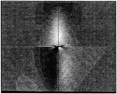
Fig. 4c Local component ![]() for τ=0.3 in the region −2≤X≤2 and −1.6≤Y≤1.6
for τ=0.3 in the region −2≤X≤2 and −1.6≤Y≤1.6
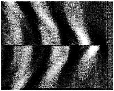
Fig. 5a Wave ![]() component for τ=0.2 in the region
component for τ=0.2 in the region ![]() and
and ![]()
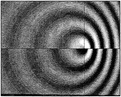
Fig.5b Wave component ![]() for τ=0.2 in the region −28≤Χω≤12 and −16≤Υω≤16
for τ=0.2 in the region −28≤Χω≤12 and −16≤Υω≤16
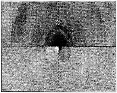
Fig. 5c Local ![]() component for τ=0.2 in the region −2≤X≤2 and −1.6≤Y≤1.6
component for τ=0.2 in the region −2≤X≤2 and −1.6≤Y≤1.6
REFERENCES
[1] B.Ponizy, F.Noblesse, M.Ba & M.Guilbaud (1994) Numerical evaluation of free-surface Green functions, Jl Ship Research 38, 193–202
[2] F.Noblesse & C.Yang (1995) Fourier-Kochin formulation of wave-diffraction-radiation by ships or offshore structures, Ship Technology Research 42, 115–139
[3] F. & X.B.Chen (1995) Decomposition of free-surface effects into wave and near-field components, Ship Technology Research 42, 167–185
[4] F.Noblesse & C.Yang (1996) Fourier representation of near-field free-surface flows, Ship Technology Research 43, 19–37
[5] F.Noblesse & X.B.Chen (1997) Far-field and near-field dispersive waves, Ship Technology Research 44, 37–43
[6] M.J.Lighthill (1958) Fourier Analysis and Generalized Functions, Cambridge University Press London, U.K.
[7] X.B.Chen & F.Noblesse (1998) Green functions and super Green functions in free-surface hydrodynamics, Colloq. on Recent Computational Developments in Steady and Unsteady Naval Hydrodynamics, Euromech 374, Poitiers, France
[8] X.B.Chen & F.Noblesse (1997) Dispersion relation and far-field waves, 12th Workshop on Water Waves and Floating Bodies 31–35, Carry-le-Rouet, France
[9] X.B.Chen & F.Noblesse (1998) Super Green functions for water waves and other dispersive waves, 3rd Intl Conf. on Hydrodynamics, Seoul, Korea
[10] F.Noblesse, X.B.Chen & C.Yang (1996) Fourier-Kochin theory of free-surface flows, 21st Symp. on Naval Hydrodynamics 120–135, Trondheim, Norway
[11] F.Noblesse, C.Yang & X.B.Chen (1997) Boundary-integral representation of linear free-surface potential flows, Jl Ship Research 41, 10–16
DISCUSSION
G.Hearn, University of Newcastle Upon Tyne, United Kingdom
Francis, your paper is extremely eloquent in its mathematical exposition. Your presentation also provides insight regarding the mathematical advantages in terms of execution of evaluation of singularity influences over sub-surfaces (panels) of appropriate surfaces or lines.
During the presentation you also referred to work by Yang & Lohner. Could you please provide exact specification of reference cited?
Adoption of your procedure will best follow complete understanding of the derivation of your super Green functions. Given the usual limitations of space in external publications could you provide details of other documents (Ph.D, internal reports) which would allow us to follow the derivations more fully? Thank you for a very interesting new approach and your insight.
AUTHORS’ REPLY
Thank you for your encouraging comments.
The far-field extension of fully nonlinear ship waves showed during the oral presentation is part of ongoing, currently unpublished, work by Chi Yang and Rainald Lohner at George Mason University. This work is expected to be reported at the 7th International Conference on Numerical Ship Hydrodynamics in a paper entitled “Fourier-Kochin extension of fully nonlinear ship waves.”
A more detailed self-contained presentation of the Fourier representation of super Green functions given in the paper will be presented in a paper entitled “Generic super Green functions” that is expected to be published in the near future.
Radiation and Diffraction of Waves in a Two-Layer Fluid
R.Yeung, T.Nguyen (University of California at Berkeley, USA)
ABSTRACT
The solution of the radiation and diffraction problem for floating bodies in a two-layer fluid of arbitrary depth is obtained using an integral-equation method. Such problems are of considerable interest for marine-vehicle operation in coastal and estuarine regions. The three-dimensional oscillatory Green function is derived, and its asymptotic expansion in the far-field is used in conjunction with Green’s theorem to obtain the symmetry relations for the added mass and damping coefficients and an analogue to the Haskind-Hanaoka relation. Added mass and damping coefficients, as well as exciting forces due to incident waves of both surface- and internal- wave modes are computed for a rectangular barge. The results indicate that density stratification can have a strong effect on the hydrodynamic characteristics of floating bodies over a wide range of frequencies.
1 INTRODUCTION
Density stratification is a common occurence in the ocean because of variation of water temperature and salinity with depth. Very often the density gradient is confined within a thin pycnocline separating two well-mixed fluid layers above and below. This pycnocline structure can be most simply modeled by a two-layer fluid where the density in each layer is constant, and the fluid is assumed to be inviscid, incompressible, and the flow irrotational. This two-layer fluid model can also be used to investigate the effects of muddy water at the bottoms of many channels and harbors on the hydrodynamic characteristics of ships. Many important hydrodynamic properties, such as added mass and damping coefficients for motions in the vertical plane, are not strongly influenced by the viscosity of the water (Yeung and Wu, 1991) or of the mud layer (Zilman et al., 1996), and the inviscid assumption provides a simple framework for addressing many physical phenomena of importance to the naval architects.
The presence of a heavier, lower fluid gives rise to internal waves on the interface between the two fluid layers. The loads on marine structures due to ambient internal waves can sometimes be quite significant. This has been documented both in field tests (Razumeenko, 1995) and in laboratory experiments (Ermanyuk and Sturova, 1994, Gavrilov et al., 1996). Despite the importance of internal waves as a source of exciting forces, there are very few theoretical studies published on this subject, and they all deal with two-dimensional cylinders. Although two-dimensional cylinders are not very practical structures, many interesting features of the wave-body interaction in a two-layer fluid have been illuminated by these studies. It is of interest to mention a parallel study for three-dimensional waves in a two-layer fluid for steady, forward motion reported in Yeung and Nguyen (1998).
Unlike waves in a uniform fluid, incident waves in a two-layer fluid can propagate with two different wave numbers k1 and k2, corresponding to the “surface-wave mode” and “internal-wave mode”, respectively (see Lamb, 1932). In the “surface-wave mode”, the amplitude of the incident waves is larger on the free surface than on the interface, but in the “internal-wave mode” the reverse is true. For the same wave frequency σ, the wavenumber k1 is smaller than k2, and the gap increases as the density difference decreases. However, regardless of the initial mode, once the incident waves impact upon the structure, waves of both modes are scattered. Thus,
wave energy can be transferred from the incident wave mode to the other mode (Sturova, 1993). In general, for the two-dimensional case, waves of wavenumbers k1 and k2 are reflected upstream and also transmitted downstream from the body. For a uniform fluid of infinite depth, it is well-known (Dean, 1948) that there is no reflection of waves of any frequency by a circular cylinder. The same property also holds true for a circular cylinder in a two-layer fluid if it is located in the infinitely deep, lower layer (Linton and McIver, 1995). However, if the cylinder is in the upper fluid layer, waves of both modes are reflected.
The transfer of energy between modes depends strongly on the density difference between the two fluid layers. When the density difference is small as in the case of fresh water laying above heavier salt water, the amount of energy transferred can be much less than 1%. If the lower layer contains fluidized mud, density ratio of 0.5 is not unrealistic. In this case, depending on the location of the body, it has been shown that as much as 20% of the energy in the incident waves of one mode can be transfered to the other mode (Linton and McIver, 1995).
In this paper, the three-dimensional, time-harmonic Green function is obtained for a two-layer fluid of arbitrary depth. This allows one to compute the wave exciting forces as well as the added mass and damping coefficients for realistic, three-dimensional bodies. Numerical results for a floating barge are presented which show the important effects of internal waves on the hydrodynamic characteristics. It should be mentioned that two-dimensional numerical results have been reported by several authors. Zilman et al. (1996) included viscosity in the formulation but concluded that, in general, viscosity is not important. This is consistent with the results for a single-layer fluid. Sturova (1994a) presented results for stationary cylinders, and Sturova (1994b) showed results for cylinders with forward velocity. In both of the latter studies, the cylinder is in the lower fluid of infinite depth, whereas in Zilman et al. (1996), the cylinder is in the upper fluid, and both fluid layers are of finite depths.
Although the time-harmonic Green function can be derived directly, in this paper, we chose to obtain the unsteady, time-dependent Green function first and use it to obtain the time-harmonic Green function. The unsteady Green function is important in itself and can be used in a time-domain formulation of the wave-body interaction problem.
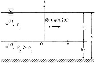
Figure 1: Coordinate system
2 UNSTEADY, TIME-DEPENDENT SOURCE
2.1 Mathematical Formulation
Consider a fixed Cartesian coordinate system Oxyz with the origin Ο located at the interface and the z-axis pointing upwards (see Fig. 1). Let’s denote the densities and depths of the upper and lower fluid layers as ρ1, h1 and ρ2, h2, respectively. For a source located at (ξ(t), η(t), ζ(t)) in the upper fluid layer, the governing equations of the velocity potentials Φ(m) are
(1)
(2)
The linearized boundary condition on the free surface is
(3)
and the conditions on the interface are
(4)
(5)
where g is the gravitational acceleration, and γ=ρ1/ρ2 is the density ratio. At the rigid bottom, the no-leak boundary condition applies,
(6)
and far away from the source, we require the velocity to vanish,
(7)
where R2=(x−ξ(t))2+(y−η(t))2. Finally, the initial conditions for Φ(m) are
(8)
(9)
2.2 Solution
We assume Φ(m) to have the following forms:
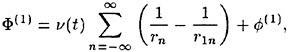
(10)
(11)
where ν(t) is the source strength and
(12)
(13)
These forms are chosen, so that the unknown potentials ![]() will satisfy the same initial conditions given by Eqns. (8) and (9). The governing equation for
will satisfy the same initial conditions given by Eqns. (8) and (9). The governing equation for ![]() is now simply the Laplace equation:
is now simply the Laplace equation:
(14)
To solve for ![]() we introduce the following transforms:
we introduce the following transforms:
(15)
(16)
(17)
Application of these transforms to Eqn. (14) yields the following equation for ![]()
(18)
where ![]() . The solutions of this equation are
. The solutions of this equation are
(19)
(20)
where the bottom condition in Eqn. (6) has been applied to obtain ![]() . The unknown coefficients
. The unknown coefficients ![]() and
and ![]() can be obtained from the remaining boundary conditions as follows.
can be obtained from the remaining boundary conditions as follows.
Substituting Φ(1) from Eqn. (10) into the free-surface boundary condition, Eqn. (3), we obtain for z=h1:
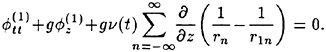
(21)
Taking the Laplace transform of the this equation and applying the initial condition, we obtain
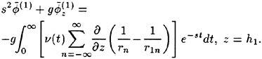
(22)
From the definition of the inverse Fourier transform in Eqn. (17), we can express ![]() in terms of à and
in terms of à and ![]() as follows:
as follows:
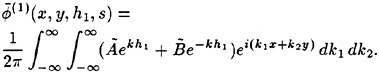
(23)
Using this expression and the well-known relationship (see Gradshteyn and Ryzhik, 1980)
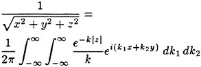
(24)
in Eqn. (23), we obtain the following equation for à and ![]()
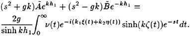
(25)
In deriving the above equation, use has been made of the formula (see Zilman and Miloh, 1995)
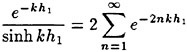
(26)
to eliminate the infinite series in Eqn. (23).
The same procedures can now be applied to the interface boundary conditions, Eqns. (4) and (5), to give
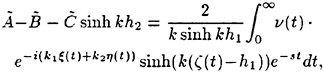
(27)
(28)
Eqns. (26), (27), and (28) form a linear system of equations which can be solved for the coefficients
Ã, ![]() and
and ![]() . Once Ã,
. Once Ã, ![]() and
and ![]() are known,
are known, ![]() can be inverted to the (x, y) space to give
can be inverted to the (x, y) space to give ![]() and
and ![]() can then be inverted to the time domain to obtain
can then be inverted to the time domain to obtain ![]() .
.
This inversion process is rather lengthy and will not be presented here. However, it is described in detail in Nguyen (1998). The velocity potentials of an unsteady, time-dependent source are given by the following final expressions:
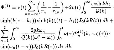
(29)
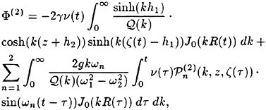
(30)
where
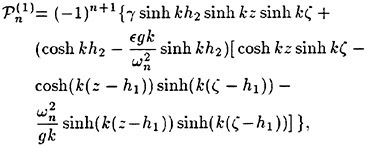
(31)
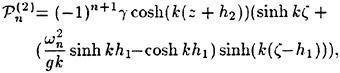
(32)
(33)
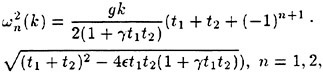
(34)
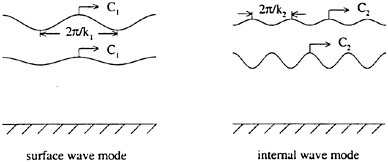
Figure 2: Two modes of propagation for waves of frequency σ
and ∈=1−γ. The functions ω1(k) and ω2(k) are the dispersion relations for the so-called “surface-wave mode” and “internal-wave mode”, respectively. We will elaborate on these two possible wave modes in a later section when we describe the velocity potentials of the incident waves. Note that when γ=1, the two-layer fluid becomes a single-layer fluid of depth h=h1+h2, and Eqn. (34) becomes
(35)
Similarly, Φ(1) and Φ(2) each becomes the velocity potential for an unsteady source in a single layer fluid (see Eqn. (13.53) of Wehausen and Laitone, 1960).
3 RADIATION AND DIFFRACTION PROBLEMS
3.1 Incident Waves in a Two-Layer Fluid of Finite Depth
Let’s denote the surface and interface elevations as ζ(1) and ζ(2), respectively, and assume the plane surface and internal waves of frequency σ propagate at an angle β relative to the positive x-axis (see Fig. 3). We can write ζ(m)(x, y, t) as
(36)
where ![]() and
and ![]() are the amplitudes of the surface and internal waves, and k is the wavenumber. The velocity potentials
are the amplitudes of the surface and internal waves, and k is the wavenumber. The velocity potentials ![]() satisfy the usual Laplace equation and also the following kinematic and dynamic conditions on the free surface
satisfy the usual Laplace equation and also the following kinematic and dynamic conditions on the free surface
(37)
(38)
and on the interface
(39)
(40)
![]() also satisfies the bottom condition
also satisfies the bottom condition
(41)
Let’s assume ![]() to have the following forms:
to have the following forms:
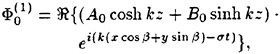
(42)
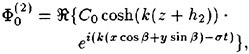
(43)
where A0, B0, and C0 are unknown coefficients. Clearly, ![]() satisfy the Laplace equation as well as the bottom condition. Substituting
satisfy the Laplace equation as well as the bottom condition. Substituting ![]() and ζ(m) into the remaining boundary conditions, Eqns. (37)–(40), we obtain A0, B0, C0 as well as the two dispersion relations given in Eqn. (34).
and ζ(m) into the remaining boundary conditions, Eqns. (37)–(40), we obtain A0, B0, C0 as well as the two dispersion relations given in Eqn. (34).
As mentioned earlier, the mode of wave propagation associated with ω1 is called the “surface-wave mode” and that associated with ω2 is called the “internal-wave mode”. Thus, incident waves of frequency σ can have two possible wavenumbers k1 and k2 given implicitly by
(44)
From Eqn. (39), the amplitude ratio ![]() is
is
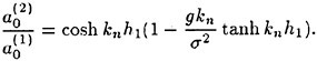
(45)
For the “surface-wave mode”, n=1, the amplitude ratio is always positive and greater than one. Thus, both surface and internal waves are in phase, and the amplitude of the surface wave is greater than the internal wave. For the “internal-wave mode”, n=2, the amplitude ratio is negative and less than one. The surface and internal waves are 180° out-of-phase, and the amplitude of the internal wave is larger than the surface wave. Fig. 2 illustrates these two possible modes of propagation for incident wave of frequency σ.
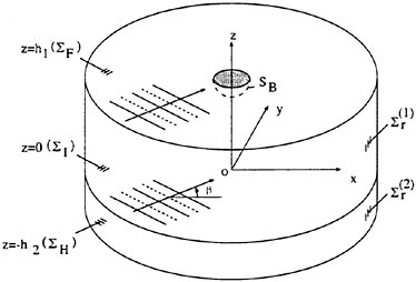
Figure 3: Radiation and diffraction problems
If the expressions for A0, B0, C0 are used in Eqns. (42) and (43), the incident wave potentials ![]() become
become
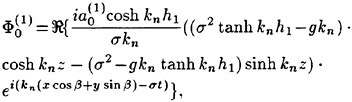
(46)
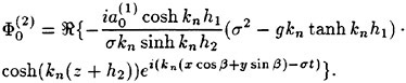
(47)
3.2 Decomposition of Potentials
Consider a rigid body oscillating in the upper fluid layer under the action of an incident wave of frequency σ (see Fig. 3). This incident wave can be of either wave mode, and its velocity potentials ![]() are given in Eqns. (46) and (47). Let’s denote the translational displacements of the body in the x, y, and z-directions as ζ1(t), ζ2(t), and ζ3(t), respectively, and the angular displacement components as ζ4(t), ζ5(t), and ζ6(t).
are given in Eqns. (46) and (47). Let’s denote the translational displacements of the body in the x, y, and z-directions as ζ1(t), ζ2(t), and ζ3(t), respectively, and the angular displacement components as ζ4(t), ζ5(t), and ζ6(t).
The velocity potentials Φ(1) and Φ(2) in the upper and lower fluid layers must satisfy the Laplace equation as well as the boundary conditions in Eqns. (3)–(6). In addition, since the body is floating in the upper fluid layer, Φ(1) must also satisfy the following linearized kinematic condition on the surface of the body in its resting position (see Wehausen, 1971):
(48)
where ![]() is the velocity of a point on the body surface, and
is the velocity of a point on the body surface, and ![]() is the unit normal vector pointing into the body.
is the unit normal vector pointing into the body.
The velocity potential Φ(m)(x, y, z, t) can be decomposed into three components:
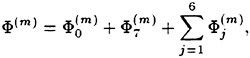
(49)
where ![]() is the incident wave potential,
is the incident wave potential, ![]() is the diffraction potential, and
is the diffraction potential, and ![]() j=1, 2,…, 6 are the radiation potentials associated with the body motions in calm water. Note that the mode of the incident wave determines
j=1, 2,…, 6 are the radiation potentials associated with the body motions in calm water. Note that the mode of the incident wave determines ![]() but it does not affect the formulation of the problem otherwise.
but it does not affect the formulation of the problem otherwise.
For time-harmonic motions, we can express ζj(t) as
(50)
where aj are the complex amplitudes of the displacements. The velocity potential Φ(m) can also be expressed in the same manner
(51)
Applying the decomposition in Eqn. (49), we can write ![]() as
as
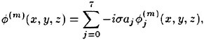
(52)
where a0=a7 is the amplitude of the incident wave. If the incident wave is of the “surface-wave mode”, ![]() and if it is of the “internal-wave mode”,
and if it is of the “internal-wave mode”, ![]() . The potential function
. The potential function ![]() can be obtained from Eqns. (45)–(47).
can be obtained from Eqns. (45)–(47).
The other potential functions ![]() j=1,…,7 satisfy the Laplace equation in their respective domains, and from Eqns. (3)–(6), the boundary conditions for
j=1,…,7 satisfy the Laplace equation in their respective domains, and from Eqns. (3)–(6), the boundary conditions for ![]() are:
are:
(53)
(54)
(55)
(56)
From Eqn. (48), we have
(57)
(58)
where n1, n2, n3 are the x, y, z-components of ![]() and n4, n5, n6 are the x, y, z-components of
and n4, n5, n6 are the x, y, z-components of ![]() . Here
. Here ![]() is the position vector of a point on the body surface, and
is the position vector of a point on the body surface, and ![]() is the position vector of the body’s center of gravity. Finally, to make the problem unique, we need to impose the appropriate radiation condition which requires the radiated and diffracted waves to be outgoing and to have the proper amplitude behavior at infinity.
is the position vector of the body’s center of gravity. Finally, to make the problem unique, we need to impose the appropriate radiation condition which requires the radiated and diffracted waves to be outgoing and to have the proper amplitude behavior at infinity.
To solve for ![]() we make use of Green’s theorem and introduce the Green function
we make use of Green’s theorem and introduce the Green function ![]()
![]() . This Green function is the velocity potential of a stationary source with oscillatory strength and will be derived in the next section. The potential function
. This Green function is the velocity potential of a stationary source with oscillatory strength and will be derived in the next section. The potential function ![]() can be expressed in terms of g(m) as
can be expressed in terms of g(m) as
(59)
where SB is the surface of the body in its resting position, and νj is the source strength distribution on SB for the jth motion. Substituting Eqn. (59) into the body kinematic boundary condition yields the following Fredholm integral equation of the second kind.
(60)
This equation can be solved for the source strength νj which is then used in Eqn. (59) to compute the potential ![]() .
.
The hydrodynamic force and moment acting on the body can be written as
(61)
(62)
where p is the fluid pressure which can be obtained from Euler’s integral as
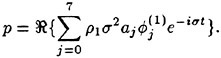
(63)
If we denote the x, y, z-components of ![]() as F1, F2, F3, and the x, y, z-components of
as F1, F2, F3, and the x, y, z-components of ![]() as F4, F5, F6, and
as F4, F5, F6, and ![]() then using Eqn. (63) we have
then using Eqn. (63) we have
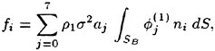
(64)
for i=1, 2,…, 6. Following the usual convention, we now define the wave exciting force per unit wave amplitude Xi as
(65)
and the “added mass” and “damping coefficients” as
(66)
In terms of these new variables, the hydrodynamic forces become
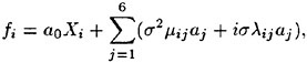
(67)
for i=1, 2,…, 6. The wave exciting force depends on ![]() and, thus, on the mode of the incident wave. The added masses and damping coefficients, however, depend only on the body geometry and not the body motion or the incident wave mode. Once Xi, μij, and λij are known, it is a simple matter to obtain the motion amplitudes aj using Newton’s second law. While all this analysis is analogous to the single-layer fluid problem, the intricacies in the two-layer problem lie in obtaining an expression for g(1).
and, thus, on the mode of the incident wave. The added masses and damping coefficients, however, depend only on the body geometry and not the body motion or the incident wave mode. Once Xi, μij, and λij are known, it is a simple matter to obtain the motion amplitudes aj using Newton’s second law. While all this analysis is analogous to the single-layer fluid problem, the intricacies in the two-layer problem lie in obtaining an expression for g(1).
3.3 Velocity Potentials of a Stationary, Oscillating Source
To solve for ![]() we first need to obtain the velocity potentials of a stationary source with oscillating strength, located in the upper fluid layer. This can most easily be accomplished if we start with the unsteady potentials Φ(m) in Eqns. (29) and (30). If we fix the source location (ξ, η, ζ) and set the source strength ν(t)=cosσt, we can then perform the t integration and take the limit as t → ∞ to obtain the desired velocity potentials (see Wehausen and Laitone, 1960). After the appropriate limiting operations, the velocity potentials G(m) of a stationary, oscillating source can be expressed as
we first need to obtain the velocity potentials of a stationary source with oscillating strength, located in the upper fluid layer. This can most easily be accomplished if we start with the unsteady potentials Φ(m) in Eqns. (29) and (30). If we fix the source location (ξ, η, ζ) and set the source strength ν(t)=cosσt, we can then perform the t integration and take the limit as t → ∞ to obtain the desired velocity potentials (see Wehausen and Laitone, 1960). After the appropriate limiting operations, the velocity potentials G(m) of a stationary, oscillating source can be expressed as ![]() where m=1 indicates the upper fluid layer, m=2 indicates the lower fluid layer, and g(m) are given by
where m=1 indicates the upper fluid layer, m=2 indicates the lower fluid layer, and g(m) are given by
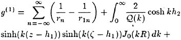
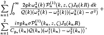
(68)
and
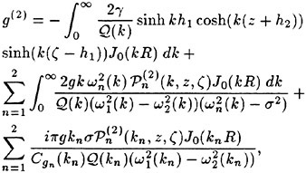
(69)
where ![]() is the group velocity for waves of the n mode.
is the group velocity for waves of the n mode.
4 RECIPROCITY RELATIONS
4.1 Radiation and Diffraction Potentials in the Far Field
Using Eqns. (68) and (69), we can obtain the following asymptotic expansion for g(m) as R → ∞ (see Nguyen, 1998):
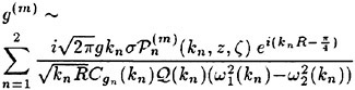
(70)
According to the above equation, for a given frequency of oscillation σ, there are two wave trains with wavenumbers k1 and k2 propagating outward from the source such that ωn(kn)=σ. The velocity potential decays at the rate of ![]() which is required for the conservation of energy.
which is required for the conservation of energy.
With the asymptotic expression for g(m) known, we can now investigate the behavior of the radiation and diffraction potentials ![]() far away from the body. The potential
far away from the body. The potential ![]() can be expressed in terms of g(m) through the following integral equation:
can be expressed in terms of g(m) through the following integral equation:
(71)
where νj is the unknown source strength on the wetted surface SB of the body. Substituting g(m)
from Eqn. (70), we have for R → ∞:
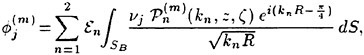
(72)
where
(73)
Next, we would like to express ![]() in terms of the so-called Kochin functions as in the single-layer fluid case (Kochin, 1940, Haskind, 1946a, b, John, 1950). These functions have been obtained for a two-layer fluid by Sturova (1994a) for the two-dimensional case. The Kochin functions depend on the geometry of the oscillating body, and in a two-layer fluid where there are two possible wave-numbers kn for a given frequency of oscillation σ, the Kochin functions Hj,n also depend on the wave mode n as well.
in terms of the so-called Kochin functions as in the single-layer fluid case (Kochin, 1940, Haskind, 1946a, b, John, 1950). These functions have been obtained for a two-layer fluid by Sturova (1994a) for the two-dimensional case. The Kochin functions depend on the geometry of the oscillating body, and in a two-layer fluid where there are two possible wave-numbers kn for a given frequency of oscillation σ, the Kochin functions Hj,n also depend on the wave mode n as well.
Before proceeding with the derivation of Hj,n, we need to convert the integrand of Eqn. (72) into a product of terms that are functions of either (ξ, η, ζ) only or (x, y, z) only. Using the expressions for ![]() in Eqns. (31) and (32), and the following definition of kn:
in Eqns. (31) and (32), and the following definition of kn:
(74)
we can rewrite ![]() as
as
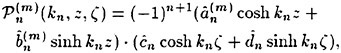
(75)
where
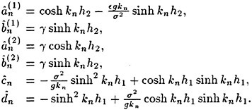
Let’s introduce the polar coordinates (r, θ) where x=R cos θ and y=R sin θ. Then when R → ∞,
(76)
Substitution of Eqns. (75) and (76) into Eqn. (72) gives the following expression for ![]() when R → ∞:
when R → ∞:
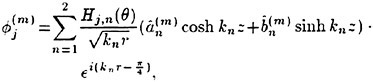
(77)
where the Kochin function Hj,n(θ) is defined as
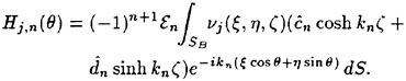
(78)
4.2 Application of Green’s Theorem
If Green’s theorem and the asymptotic expression of ![]() in Eqn. (77) are now used, it is possible to systematically derive the various reciprocity relations pertaining to the interaction of waves with a floating body. This has been done by Newman (1976) for a single-layer fluid for both two-dimensional and three-dimensional cases. Two-dimensional relations for a two-layer fluid of infinite depth have been obtained by by Wu (1992), Sturova (1994a), and Linton and McIver (1995). In this paper, we will not attempt to derive all the possible relations for the three-dimensional case. Instead, we will focus only on the symmetry of the added mass and damping coefficients and on an analogous Haskind-Hanaoka relation for the exciting forces.
in Eqn. (77) are now used, it is possible to systematically derive the various reciprocity relations pertaining to the interaction of waves with a floating body. This has been done by Newman (1976) for a single-layer fluid for both two-dimensional and three-dimensional cases. Two-dimensional relations for a two-layer fluid of infinite depth have been obtained by by Wu (1992), Sturova (1994a), and Linton and McIver (1995). In this paper, we will not attempt to derive all the possible relations for the three-dimensional case. Instead, we will focus only on the symmetry of the added mass and damping coefficients and on an analogous Haskind-Hanaoka relation for the exciting forces.
To apply Green’s theorem to a two-layer fluid of finite depth, we introduce the closed surfaces Σ(1) and Σ(2) as shown in Fig. 3. The surface Σ(1) contains only the upper fluid and consists of the body surface SB, the circular cylindrical surface ![]() of radius r, extending from the free surface to the interface, the circumscribed portion of the free surface exterior to the body ΣF, and the circumscribed portion of the interface ΣI. The second closed surface Σ(2) contains only the lower fluid. It consists of the circular cylindrical surface
of radius r, extending from the free surface to the interface, the circumscribed portion of the free surface exterior to the body ΣF, and the circumscribed portion of the interface ΣI. The second closed surface Σ(2) contains only the lower fluid. It consists of the circular cylindrical surface ![]() extending from the interface to the fluid bottom, the surface ΣI, and the circumscribed bottom ΣH.
extending from the interface to the fluid bottom, the surface ΣI, and the circumscribed bottom ΣH.
Applying Green’s second identity to a pair of potentials ![]() and
and ![]() over Σ(1) we have
over Σ(1) we have
(79)
where n is the normal direction out of the fluid domain. Since ![]() and
and ![]() satisfy the free surface boundary condition, Eqn. (53), the integral over ΣF vanishes. Next, to evaluate the integral over ΣI, we introduce the corresponding pair of potentials in the lower layer,
satisfy the free surface boundary condition, Eqn. (53), the integral over ΣF vanishes. Next, to evaluate the integral over ΣI, we introduce the corresponding pair of potentials in the lower layer, ![]() and
and ![]() . The potentials
. The potentials ![]() and
and ![]() satisfy the kinematic and dynamic boundary conditions on the interface, Eqns. (54) and (55), and from these conditions
satisfy the kinematic and dynamic boundary conditions on the interface, Eqns. (54) and (55), and from these conditions
we obtain:
(80)
Similarly, for ![]() and
and ![]() we have
we have
(81)
Combining Eqns. (80) and (81), we arrive at
(82)
for z=0. This equation relates the potentials in the upper fluid layer to those in the lower layer. Next, we apply Green’s second identity to ![]() and
and ![]() over Σ(2) to obtain
over Σ(2) to obtain
(83)
Since ![]() and
and ![]() satisfy the bottom boundary condition, the integral over ΣH vanishes, and Eqn. (83) becomes
satisfy the bottom boundary condition, the integral over ΣH vanishes, and Eqn. (83) becomes
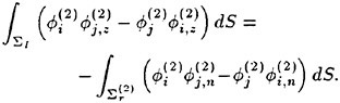
(84)
Using Eqns. (82) and (84), we can rewrite Eqn. (79) as
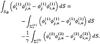
(85)
To evaluate the integrals over ![]() we note that when r → ∞, the velocity potentials can be approximated by the asymptotic expansion given in Eqn. (77). Substituting this expansion into Eqn. (85), we have
we note that when r → ∞, the velocity potentials can be approximated by the asymptotic expansion given in Eqn. (77). Substituting this expansion into Eqn. (85), we have
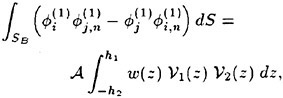
(86)
where A is some known function, and
(87)
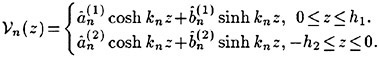
To show that the integrals in Eqn. (86) vanishes, we now introduce the following interface Sturm-Liouville problem. This problem is encountered when the boundary-value problem described in Eqns. (37)–(41) is solved using separation of variables. If we let ![]() then we obtain the following interface Sturm-Liouville problem for
then we obtain the following interface Sturm-Liouville problem for ![]()
(88)
and the boundary conditions for ![]() are
are
(89)
(90)
(91)
(92)
The solution of this Sturm-Liouville problem can easily be obtained. The eigenvalues are kn, n=1, 2, where kn are defined in Eqn. (35). The eigenvectors,
(93)
and the weighting functions w(z) can be shown to be given by Eqn. (87) (see Wylie and Barrett, 1995). Thus, the right-hand side integral vanishes because of the orthogonality of the eigenvectors Vn, and Eqn. (86) becomes
(94)
4.3 Symmetry of Added Mass and Damping Coefficients
Since Eqn. (94) is the same as that for a single-layer fluid, the proof that the added mass and damping coefficients are symmetric follows the same argument as in that case (see Wehausen, 1971). Applying Eqn. (94) to the two radiation potentials ![]() and
and ![]() we obtain
we obtain
(95)
By using the kinematic boundary condition on SB, Eqn. (95) becomes
(96)
From the definitions of the added mass and damping coefficients, it’s easy to see that μi,j=μj,i and λi,j=λj,i.
4.4 Analogue of Haskind-Hanaoka Relation for a Two-Layer Fluid
In a single-layer fluid, the Haskind-Hanaoka relation allows one to compute the exciting forces from the radiation potentials and the incident wave potential. Thus, it is not necessary to solve for the diffraction potential itself if one is only interested in the forces. In a two-layer fluid, an analogous relation exists which can be derived using Eqn. (94). The derivation follows the same line of argument as in the single-layer fluid case (see Wehausen, 1971). The wave exciting force can be computed as
(97)
or in terms of the far-field potentials
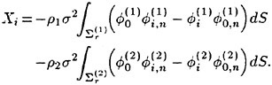
(98)
Thus, one can compute Xi without having to solve for the diffraction potential ![]() . Eqn. (98) has an advantage over Eqn. (97) in that the asymptotic expression for
. Eqn. (98) has an advantage over Eqn. (97) in that the asymptotic expression for ![]() in Eqn. (77) can be used to evaluate Xi. However, it does require the computation of both
in Eqn. (77) can be used to evaluate Xi. However, it does require the computation of both ![]() and
and ![]() .
.
5 NUMERICAL RESULTS
5.1 Numerical Evaluation of g(1)
In this paper, we are concerned with the motion of bodies floating in the upper fluid layer and not intersecting the fluid interface. Thus, we only need to evaluate g(1) and not g(2). These two functions, however, have similar forms, and the same method can be used for their evaluation.
The first term of g(1), Eqn. (68), represents an infinite array of Rankine sources and sinks. It is evaluated using the method presented in Newman (1992) which employs Fourier series and Chebyshev expansion. When R/h<1, the integrals of g(1) are computed using an adaptive quadrature with Simpson’s rule (see Conte and Boor, 1980). For the principal-valued integrals, the poles kn are obtained using Newton’s method, and these singularities are removed using the procedure in Endo (1987) before the numerical integration is performed. When R/h>1, direct numerical integration is inefficient, and a series expansion of g(1) is used for numerical evaluation. This series expansion is analogous to the series obtained by John (1950) for a single-layer fluid, and as in that case, the series converges exponentially and is more efficient than numerical integration.
5.2 Integral-Equation Solution
Numerical results are obtained for a floating barge, modeled here as a rectangular box. A brief review of integral-equation formulation may be found in Yeung (1982). Here, the low-order panel method of Hess & Smith (1964) is used for simplicity. Higher-order panel method such as Hamilton & Yeung (1997) can be easily adopted.
To solve Eqn. (60), we approximate the body surface by Ν plane, quadrilateral panels. For the rectangular box in our example, this geometrical discretization is adequate and will not leave any gaps between adjacent panels. For each panel p, we assume the source strength νj,p to be constant and define the control point (xp, yp, zp) as the null point of the panel (see Hess and Smith, 1964). Applying Eqn. (60) to each panel p will yield the following system of linear equations
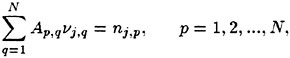
(99)
where nj,p is the component nj evaluated at the control point of panel p, and the element of Ap,q is defined as
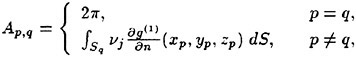
(100)
where Sq is the surface area of panel q. To perform the integration over Sq, we use the Gaussian quadrature with 3 points in each direction for a total of 9 points for each panel. This system of equations is then solved using the direct method of Gaussian elimination. The potential ![]() which is also constant over each panel p, is
which is also constant over each panel p, is
evaluated at the control point as
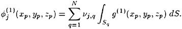
(101)
The wave exciting forces and the added mass and damping coefficients are computed in the same manner as well.
5.3 Floating Barge in a Two-Layer Fluid of Finite Depth
The wave exciting forces and hydrodynamic coefficients are computed for a floating barge, modeled here as a rectangular box. The dimensions of the box are chosen so that comparison with the numerical results of Endo (1987) for a single-layer fluid is possible. The length L of the box is 90 m, and its draft D is 40 m. A total number of 192 panels is used to discretize the surface of the box. The results obtained agree with those using 432 panels, thus, verifying the convergence of the numerical solution.
To study the effects of the density ratio γ, we obtain the solutions for γ=1, 0.9, 0.7, 0.1. For these runs, the depths of the fluid layers are fixed, h1=1.2D and h2=0.4D. When γ=1, the two-layer fluid becomes a single-layer fluid of depth h=h1+h2=1.6D, and the results can be compared with those of Endo (1987) for the same depth. As γ approaches zero, i.e., ρ2 becomes infinitely large, the lower fluid behaves more like a rigid block, and we would expect the results to approach those for a single-layer fluid of depth h1, the depth of the upper fluid layer. To illustrate this behavior, we include the results for a single-layer fluid of depth h1 in the plots as well.
Figs. 4–9 show the added mass and damping coefficients for surge, heave, and pitch. The hydrodynamic coefficients for yaw were computed but are not presented here. The results for γ=1 and h=1.6D agree quite well with those of Endo (1987). Also, the results for γ=0.1 approximate those for a single-layer fluid of depth h=1.2D as expected. The results for γ=0.7, 0.9 are in between these two limits, and when compared to the single-layer fluid case, they illustrate the effects of the internal waves on the hydrodynamic coefficients of the box. At high frequencies, these results are similar as those for a single-layer fluid which indicate that the internal waves are relatively unimportant. However, at lower frequencies, dramatic differences in the hydrodynamic coefficients can be seen, and they can be attributed to the presence of the internal waves.
For the same frequency of oscillation σ, the wavelength λ1 of the surface-wave mode is larger than the wavelength λ2 of the internal-wave mode. At high frequencies, the wavelength λ2 is too small for the internal waves to be important. Also, the difference λ1 and λ2 increases as γ increases. This means that as the density difference becomes very small, the effects of the internal waves are concentrated within a smaller range of low frequencies. This can be seen in Fig. 7 where the heave damping coefficient for γ=0.9 exhibits a significant peak over a range of lower frequencies.
Figs. 10–15 show the magnitude of the surge, heave, and pitch exciting forces due to both the surface-wave mode and the internal-wave mode. These forces are normalized by the amplitude a0 of the incident wave (see Eqn. (67)). For the surface-wave mode, a0 represents the amplitude of the incident surface wave, and similarly, for the internal-wave mode, a0 is the amplitude of the incident internal wave. The surge and heave exciting forces for the surface-wave mode do not differ significantly from those due to surface waves in a single-layer fluid. The pitch exciting moment, however, has larger oscillation especially for γ=0.7 and 0.9. The exciting forces due to the internal-wave mode, which does not exist in a single-layer fluid, exhibit many peaks and valleys. These peaks and valleys and the oscillations seen earlier in the added mass and damping coefficients are caused by the interaction between internal waves generated by the opposite edges of the rectangular box. The nondimensional magnitude of the exciting forces increases as γ decreases. This can be explained by the larger potential energy per unit amplitude of the incident internal waves when γ is small.
Figs. 16–21 show the motion amplitudes for both wave modes. Fig 18, in particular, shows the heave amplitude for the surface-wave mode and indicates that the presence of the lower fluid layer reduces the heaving motion. Fig. 21 shows the pitch amplitude for the internal-wave mode. Large pitching motion can be exited by the internal waves.
The effects of fluid depths on the forces and hydrodynamic coefficients were also investigated. However, owing to space limitation, these results are not presented here. They can be found in Nguyen (1998).
6 CONCLUSIONS
In this paper, the unsteady, time-dependent Green functions and the time-harmonic Green functions are derived for a two-layer fluid of finite depth. The latter Green functions are then used to solve the radiation and diffraction problems associated with the interaction of waves with floating bodies. By using Green’s theorem, the symmetry relations for the added mass and damping coefficients as well as an analogue to the Haskind-Hanaoka relation are established. Numerical results for a rectangular box are presented. They show the strong influence of the internal waves on the hydrodynamic coefficients over a wide range of frequencies. For incident waves of the surface-wave mode, the heaving motion is reduced by the presence of the lower fluid layer. However, large pitching motion can be excited by incident waves of the internal-wave mode.
Acknowledgements
We are pleased to acknowledge the support of the Office of Naval Research under Grant No. N00014–91–J1614 and N00014–95–1–0980. Partial support from the Shell Foundation is also gratefully acknowledged.
References
[1] Conte, S.D. and Boor, C. (1980). Elementary Numerical Analysis, McGraw-Hill, New York.
[2] Dean, W.R. (1948). “On the reflection of surface waves by a submerged circular cylinder,” Proc. Camb. Phil. Soc., 44, pp. 483–491.
[3] Endo, H. (1987). “Shallow-water effect on the motions of three-dimensional bodies in waves,” Journal of Ship Research, 31, pp. 34–40.
[4] Ermanyuk, E. and Sturova, I. (1994). “Effects of Regular Waves on the Body Submerged in a Stratified Fluid,” Proceedings of the 20th Symposium on Naval Hydrodynamics, Santa Barbara, CA.
[5] Gavrilov, N., Ermanyuk, E. and Sturova, I. (1996). “The forces exerted by internal waves on a restrained body submerged in a stratified fluid,” Proceedings of the 21st Symposium on Naval Hydrodynamics, Trondheim, Norway.
[6] Gradshteyn, I.S. and Ryzhik, I.M. (1980). Table of Integrals, Series, and Products, Academic Press, Orlando.
[7] Hamilton, J.A. and Yeung, R.W. (1997). “Shell-function solutions for three-dimensional nonlinear body motion problems,” Schiffstechnik, 44, no. 1, pp. 62–70.
[8] Haskind, M.D. (1946a). “The hydrodynamic theory of ship oscillations in rolling and pitching,” Prikl. Mat. Mekh., 10, pp. 33–66.
[9] Haskind, M.D. (1946b). “Waves arising from oscillation of bodies in shallow water,” Prikl. Mat. Mekh., 10, pp. 475–480.
[10] Hess, J.L. and Smith, A.M.O. (1964). “Calculation of nonlifting potential flow about arbitrary three-dimensional bodies,” Journal of Ship Research, 8, pp. 22–44.
[11] John, F. (1950). “On the motion of floating bodies,” Comm. Pure Appl. Math, 3, pp. 45–101.
[12] Kochin, N.E. (1940). “The theory of waves generated by oscillations of a body under the free surface of a heavy incompressible fluid,” Uchenye Zapiski Moskov. Gos. Univ., 46, pp. 85–106.
[13] Lamb, H. (1932). Hydrodynamics, 6th ed., Dover Publication Inc., New York.
[14] Linton, C.M. and McIver, M. (1995). “The interaction of waves with horizontal cylinders in two-layer fluids,” Journal of Fluid Mechanics, 304, pp. 213–229.
[15] Newman, J.N. (1976). “The interaction of stationary vessels with regular waves,” Proceedings of the 11th Symposium on Naval Hydrodynamics, London, England.
[16] Newman, J.N. (1992). “The approximation of free-surface Green functions,” Wave Asymptotics, Cambridge University Press, Cambridge, England.
[17] Nguyen, T.C. (1998). “Green’s functions for a two-layer fluid of finite depth,” Ph. D. thesis, University of California, Berkeley.
[18] Razumeenko, Y.V. (1995). “Changeability of hydrophysics ocean fields; Problems of manoeuvrability of submerged objects in real ocean,” International Symposium on Ship Hydrodynamics, St. Petersburg, Russia.
[19] Sturova, I.V. (1993). “Scattering of surface and internal waves on submerged body,” Computational Technology, Novosibirsk, 2, pp. 30–45.
[20] Sturova, I.V. (1994a). “Plane problem of hydrodynamic rocking of a body submerged in a two-layer fluid without forward speed,” Fluid Dynamics, 29, pp. 414–423.
[21] Sturova, I.V. (1994b). “Hydrodynamic forces on a submerged cylinder advancing in waves of two-layer fluids,” Proceedings of the 9th International Workshop on Water Waves and Floating Bodies, Kuju, Japan.
[22] Wehausen, J.V. and Laitone, E.V. (1960). “Surface waves,” Handbuch der Physik, 9, Springer, Berlin.
[23] Wehausen, J.V. (1971). “The motion of floating bodies,” Annual Review of Fluid Mechanics, 3, pp. 237–268.
[24] Wylie, C.R. and Barrett, L.C. (1995). Advanced Engineering Mathematics, 6th ed., McGraw-Hill, New York.
[25] Wu, J.H. (1992). “The second order wave loads on bodies in stratified ocean,” Proceedings of the 7th International Workshop on Water Waves and Floating Bodies, Val de Reuil, France.
[26] Yeung, R.W. (1982). “Numerical methods in free surface flows,” Annual Review of Fluid Mechanics, 14, pp. 395–442.
[27] Yeung, R.W. and Nguyen, T. (1998). “Waves generated by a moving source in a two-layer ocean of finite depth,” Journal of Engineering Math, to be published.
[28] Yeung, R.W. and Wu, C.F. (1991). “Viscosity effects on the radiation hydrodynamics of horizontal cylinders,” ASME Journal of Offshore Mechanics and Arctic Engineering, 113, pp. 334–343.
[29] Zilman, G. and Miloh, T. (1995). “Hydrodynamics of a body moving over a mud layer—Part I: wave resistance,” Journal of Ship Research, 39, pp. 194–201.
[30] Zilman, G., Kagan, L. and Miloh, T. (1996). “Hydrodynamics of a body moving over a mud layer—Part II: added-mass and damping coefficients,” Journal of Ship Research, 40, pp. 39–45.
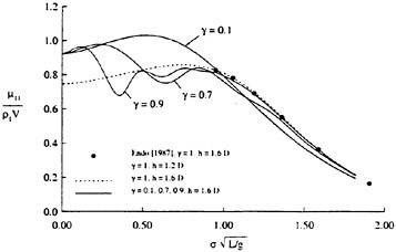
Figure 4: Surge added mass of a rectangular box, h1=1.2D, h2=0.4D
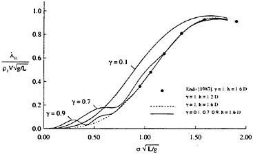
Figure 5: Surge damping coefficient of a rectangular box, h1=1.2D, h2=0.4D
Figure 6: Heave added mass of a rectangular box, h1=1.2D, h2=0.4D
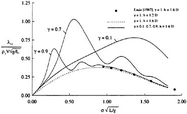
Figure 7: Heave damping coefficient of a rectangular box, h1=1.2D, h2=0.4D
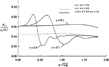
Figure 8: Pitch added moment of inertia of a rectangular box, h1=1.2D, h2=0.4D
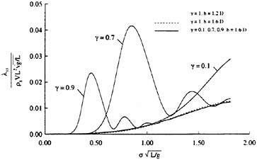
Figure 9: Pitch damping coefficient of a rectangular box, h1=1.2D, h2=0.4D
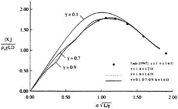
Figure 10: Magnitude of surge exciting force, surface-wave mode (n=1), h1=1.2D, h2=0.4D, β=0
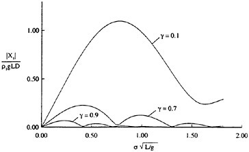
Figure 11: Magnitude of surge exciting force, internal-wave mode (n=2), h1=1.2D, h2=0.4D, β=0
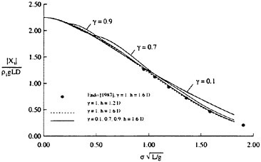
Figure 12: Magnitude of heave exciting force, surface-wave mode (n=1), h1=1.2D, h2=0.4D, β=0
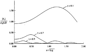
Figure 13: Magnitude of heave exciting force, internal-wave mode (n=2), h1=1.2D, h2=0.4D, β=0
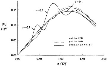
Figure 14: Magnitude of pitch exciting moment, surface-wave mode (n=1), h1=1.2D, h2=0.4D, β=0
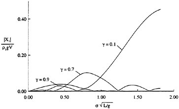
Figure 15: Magnitude of pitch exciting moment, internal-wave mode (n=2), h1=1.2D, h2=0.4D, β=0
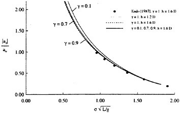
Figure 16: Surge amplitude, surface-wave mode (n=1), h1=1.2D, h2=0.4D, β=0
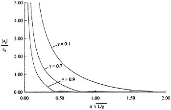
Figure 17: Surge amplitude, internal-wave mode (n=2), h1=1.2D, h2=0.4D, β=0
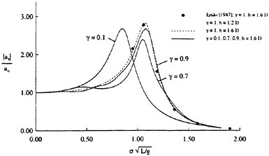
Figure 18: Heave amplitude, surface-wave mode (n=1), h1=1.2D, h2=0.4D, β=0
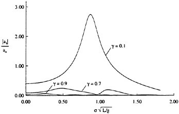
Figure 19: Heave amplitude, internal-wave mode (n=2), h1=1.2D, h2=0.4D, β=0

Figure 20: Pitch amplitude, surface-wave mode (n=1), h1=1.2D, h2=0.4D, β=0
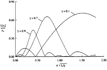
Figure 21: Pitch amplitude, internal-wave mode (n=2), h1=1.2D, h2=0.4D, β=0
DISCUSSION
G.Hearn
University of Newcastle Upon Tyne, United Kingdom
Thank you for a very interesting and mathematically beautiful paper. Demonstration of the reduction of your results to those of Wehausen and Laitone for the case of p1–p2, together with the symmetry of the reactive coefficients and the extension of the Haskind-Hanoaka relationship, provides additional eloquence. In short I thoroughly enjoyed your paper.
The application of the analysis is readily appreciated. To what extent could the analysis be extended in terms of p2 varying, to represent the stratification one might find in the muddy bottom?
AUTHORS’ REPLY
Thank you, Prof. Hearn, for your kind remarks and generous comments on our work. The development of the necessary Green functions in this paper was certainly made easier by assuming the density constant in each of the layers. Analytical expressions will be difficult to obtain if the variation in density is arbitrary within any given layer. There is a possibility that a linear variation or an exponentially decaying variation may still lead to analytical results.
Nonlinear Simulation of Breaking Waves with Spilling Breakers by a Boundary Integral Method
D.Sadovnikov (Krylov Shipbuilding Research Institute, Russia)
G.Trincas (University of Trieste, Italy)
Abstract
This paper describes a new generalized method for simulating free-surface flows with breaking, based on fully nonlinear wave potential theory. The method may reproduce wave profiles accurately provided the breaking phenomenon is modelled properly. To this end, the limited zone of the free surface where wave breaking occurs is substituted by a fictitious solid plate, following applications of the Riaboushinsky cavity termination model on the ending part of a cavity past a hydrofoil. This model is capable to take into account fluid energy dissipation processes in the breaker. It is demonstrated that the hydrostatic model of a spilling breaker as defined by Cointe and Tulin [1] on the basis of Duncan’s systematic experiments [2], is a particular case of the proposed model.
In the present work the breaking phenomenon of periodic Stokes’ limiting waves in deep water is studied from a numerical point of view. A set of results ranging from non-breaking solution up to the strongest breaking solution is discussed. Comparison between theoretical results and available experimental data shows good qualitative and quantitative agreement between the strongest breaking solution and the incipient steady wave breaking past a hydrofoil. It is also shown that the calculated free surface with the largest breaker and the smallest following waves downstream more probably emulate the natural phenomenon.
1 Introduction
Although accurate prediction of the flow with breaking waves is of paramount importance for many practical applications in shipbuilding, this phenomenon became a subject of intensive research only in the last thirty years. Various applicativ approaches of fully nonlinear wave theory in combination with viscous turbulent flow theory were derived to tackle this complicate problem. While experiments have dealt with both breaking and non-breaking waves, most CFD approaches consider non-breaking situations only, since limited knowledge of the mechanism of breaking waves still hampers adequate physical identification of the problem at hand and many numerical difficulties arise when the free surface is subject to large deformations.
Mason [3] classified two basic types of breaking waves, namely, spilling breakers and plunging breakers. The first type of breaking is characterized by areas of aerated water on the forward wave face impinging on the underlying wave from the crest and overturning to its leading edge, as it may be observed in deep ocean waves and around surface ships. Plunging breakers look like jets falling down from the wave crest to the front wave face like waves on a sloping beach. Although this classification is based on outward appearance of breaking waves, it has a deeper implication: fluid flows with plunging breakers are always strongly unsteady, whereas free-surface flows with spilling breakers are slightly unsteady or can be quasi-steady as it happens in front of a floating body or past a submerged body moving at constant speed.
Theoretical investigations of plunging and spilling breakers were carried out by means of different approaches and methods in the past two decades. Breaking waves with plunging breakers have been considered as non-dissipative overturning waves, and unsteady nonlinear wave theory has been used for their numerical computations [4, 5].
When investigating spilling breakers, viscous processes should be anyway taken into account since energy dissipation plays the leading role. The problem becomes significantly more difficult due to the
turbulent character of the flow with breaking waves at the scales which occur in nature. The first attempt to theoretically investigate spilling breakers was made by Longuet-Higgins [6] who associated the spilling breaker with a turbulent wedge and assumed the existence of a stagnation point at its leading edge. But this assumption was not confirmed by the experimental work of Banner and Phillips [7], who observed a stagnation point at the breaking wave crest, a rolling eddy on the face of the breaking wave and a viscous turbulent wake downstream of the breaker. The second model of a spilling breaker, proposed by Longuet-Higgins and Turner [8] to evaluate parameters of sea breaking waves, implied the existence of a gravity current riding down the front face of the wave.
So far, the most important contribution to physical understanding of spilling breakers was given by Duncan [2] who towed a two-dimensional submerged hydrofoil in a small towing tank at different values of hydrofoil speed and depth of submergence. The length and height of both the broken wave and the following waves were measured systematically to define relationships relating breaker’s geometric parameters and wave dimensions. He observed not only a zone of recirculated aerated water and a turbulent wake past the hydrofoil, but demonstrated that shear stresses, which produce a turbulent wake downstream, exist between the breaker and the underlying wave and sustain the spilling breaker on the front wave slope. He evaluated also the density of aerated fluid in the breaker indirectly, which resulted to be about 60% of the water density.
Duncan’s experiments gave rise to a theory of steady spilling breakers developed by Cointe and Tulin [1] and Tulin and Cointe [9]. They applied an idealization of the classical mixing turbulent layer at the onset point of the breaker and utilized extensive experimental data to identify relationships between amplitude and length of the following waves, breaker’s size and parameters of the viscous turbulent wake. They found that two types of breaking are possible, i.e. weak and strong breaking, then deriving that only strong breaking solution with a large breaker is stable and may take place. Finally, they proposed a hydrostatic model of spilling breaker and applied it to potential calculations based on a linear wave theory.
In the last decade, there has been remarkable progress in the nonlinear simulation of large-amplitude surface waves by numerical methods Many researchers (Miyata [10], Mori and Shin [11], Lungu and Mori [12], Kawamura et al. [13], Trincas [14], Kang [15]) have solved RANS equations directly by applying finite-difference or finite-volume schemes in order to simulate free-surface flows with breaking. Although some results seem very promising when wave breaking is induced by shallowly submerged bodies, it should be pointed out that all published numerical simulations have been carried out at low Reynolds numbers where turbulence stresses are not so relevant. Moreover, most of these methods use an overpressure superposition on the free surface when the transition to sub-breaking seems to take place, then switching the numerical scheme into that representative of the fully turbulent flow for which available turbulence models are still inadequate. The main limitation of all aforesaid methods consists in incorrect description of the breaking area at high Reynolds numbers typical of sea waves and marine vehicles.
It is authors’ opinion that the most effective way to investigate free-surface flows with breaking waves is to create simplified breaker’s models capable to describe the most important features of the physical process and to apply them to potential calculations by boundary integral equations of different type. The present paper discusses such an approach while improving previous studies by Sadovnikov [16, 17], who offered a simplified way for modelling the zone of free-surface breaking similar to Ivanov’s application of some cavity termination model to the ending part of a cavity [18]. In this work the model of steady spilling breakers has been combined with a numerical technique based on a fully nonlinear potential theory which implicitly includes viscous effects. The free-surface shape of periodic Stokes’ limiting waves breaking has been simulated accurately enough. Although the hydrostatic flat-topped model of a spilling breaker [9] is fully suitable to be introduced into the new generalized approach, results show that more adequate breaker’s models are to be expected from analysis of further experimental measurements.
2 Steady models of a spilling breaker
Wave breaking is a very complicated phenomenon because it is substantially unsteady and is always coupled with energy dissipation in the fluid. A classic example of a dissipative free-surface flow is a cavity after a body (Fig. 1) whose ending part is
unsteady even when the flow velocity is constant at infinity upstream. The fluid flow at the ending part of the cavity is dissipative and, therefore, rather difficult to be numerically evaluated in full detail. In the theory of cavitating flows [18] this problem is traditionally avoided by applying special cavity termination models. One of the most popular is the so-called generalized Riaboushinsky cavity termination model, where the cavity is closed by some solid fictitious body; for instance, by a vertical plate in the case of supercavitating flow around a hydrofoil (Fig. 1b).
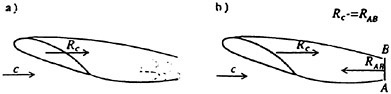
Figure 1: Cavitating flow past a hydrofoil
Since pressure on the fictitious body is not equal to the one on the free surface, a force appears on the plate. Projection RAB of this force on the incoming flow direction is equivalent to the cavitational resistance Rc of the initial body, say the hydrofoil. The composed body, consisting of a part of the initial body surface, of the cavity boundary and of the fictitious body surface, has nonzero wave resistance according to the d’Alembert paradox. Therefore, it may be concluded that a complicated unsteady dissipative phenomenon like cavitation can be investigated by means of steady potential theory.
2.1 Simplified general approach to simulate spilling breakers
In the present paper the same approach is applied to investigate breaking waves with spilling breakers. Like in the generalized Riaboushinsky cavity termination model, the free-surface region where wave breaking occurs is substituted by a solid plate of arbitrary shape (Fig. 2).
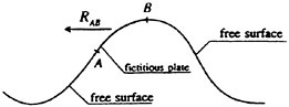
Figure 2: Wave breaking region modelled by a plate
The horizontal projection (RAB) of the force produced by the difference between the pressure on the plate and the atmospheric pressure, approximately describes the complicate dissipative processes in the breaker. Different applications of this modelling with a fictitious plate are shown in Figure 3.
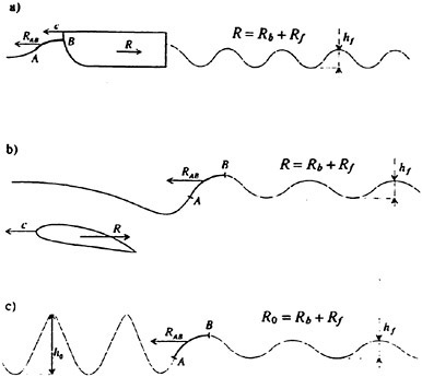
Figure 3: Different applications of a fictitious plate
If bow wave breaking occurs in front of a body moving on the water surface (Fig. 3a) or breaking wave arises past a towed shallowly submerged body (Fig. 3b), then the horizontal force RAB on the fictitious plate AB is equal and opposite to the resistance Rb due to wave breaking (Rb=−RAB). Following the momentum theorem, the wave resistance R of the moving body is the sum of resistance Rf due to following waves and resistance Rb
(1)
In the case of free progressive waves (Fig. 3c), breaking of one wave results in decreasing of the height of the waves downstream, and the resistance equation takes the form
(2)
In equations (1) and (2), the resistance associated to the following waves and incoming waves can be expressed respectively as
(3)
where c is the propagation speed of the waves; ![]() and
and ![]() denote the wave energy per unit of wave length and the energy propagation speed of the wave train following the breaking wave, respectively;
denote the wave energy per unit of wave length and the energy propagation speed of the wave train following the breaking wave, respectively; ![]() and
and ![]() signify the same characteristics for the incoming waves.
signify the same characteristics for the incoming waves.
This simplified general approach makes it possible to investigate free-surface flows with breaking waves by means of steady potential theory. But the shape and size of the fictitious plate AB simulating the wave breaking area, are unknown. Correct determination of these parameters implies experimental identification of adequate models for the decription of the wave breaking area.
2.2 Breaker with vertical plate
Like in the case of the cavity termination model for supercavitating flows past a hydrofoil (Fig. 1b), the model of breaking wave may be introduced in which the fictitious solid plate AB is flat and vertical, and extends as far as the wave crest (Fig. 4). The crest point Β of the breaking wave is a stagnation point; the free surface should be horizontal there (ω1=90°) as it occurs past a blunt body [19].
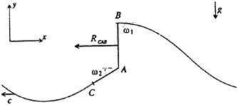
Figure 4: Breaking wave model with two plates
But unlike cavitating flows of weightless fluids, it is necessary to include an additional inclined plate AC since the free surface of a gravity steady potential flow can not be vertical. This solution was confirmed by Maklakov [20], who investigated two-dimensional free-surface flows behind inclined rectilinear plates and found that a steady free surface does exist only past a plate inclined less than 30°. That is why the inclination angle of the additional plate was set as ω2≤30° in Sadovnikov’s model of a spilling breaker [16].
This model that looks like the Riaboushinsky cavity termination model has some disadvantages; among the other things, it gives the same values of the crest elevation over the undisturbed water level for both the breaking wave and Stokes’ limiting wave, though the former is always lower than the latter according to all experimental data. Moreover, this model is not suitable for numerical computations since it assumes the simultaneous existence of two singular points A and B. Nevertheless, application of this model [17] showed its efficiency in evaluating the overall flow pattern outside the zone of the free-surface breaking.
2.3 Hydrostatic model of a spilling breaker
In accordance with Duncan’s experimental data [2], a spilling breaker has a distinctive shape characterized by two main features: i) the breaker’s height rapidly grows at its lowest point where it touches the front slope of the breaking wave; ii) the upper surface of the breaker reaches the wave crest where it becomes horizontal. Therefore, the breaker’s shape can be approximated by a right-angled triangle with catheti h* and l* which are the total height and length of the breaker, respectively (Fig. 5a).
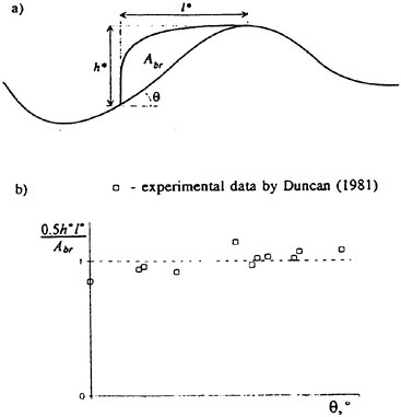
Figure 5: Evaluation of breaker’s shape
Figure 5b illustrates the ratio of the area of the triangle 0.5h*l* to the experimental area of the breaker Αbr versus the wave slope θ under the breaker. The velocity of the recirculating motion of the aerated fluid in the breaker is much lower than the speed of the propagating breaking wave. Therefore, also the dynamic pressure acting on the wave beneath the breaker is relatively small, being approximately 10% lower than the hydrostatic pressure of the breaker. Tulin and Cointe [9] showed that also the influence of the viscous turbulent wake on the flow pattern, caused by shear stresses between the breaker and the wave beneath, is relatively small but noticeable. In fact, the length of the following waves downstream of the breaking wave is
slightly reduced (less than 10%) with respect to the length of conventional progressive waves with the same phase speed. Therefore, a hydrostatic model of a spilling breaker can be formulated (Fig. 6) as a stagnant zone of the motionless aerated fluid with a lower density ρb=0.6ρ [2]. This region has the upper shape like a flat-topped right-angled triangle and reaches the breaking wave crest. In fact, this model substitutes the area of wave breaking by a curved fictitious plate AB placed between the breaker and the underlying wave
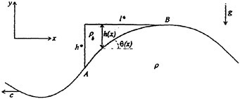
Figure 6: Hydrostatic model of a spilling breaker
The breaker exercises its influence on the fictitious plate AB by a hydrostatic pressure
(4)
where g is the gravity acceleration and h(x) is the local height of the breaker. This overpressure has a suppressive effect on the underlying wave. The horizontal force Rb applied on the fictitious plate AB and associated with dissipative processes, depends on the size of the breaker as well as on the wave slope θ on the dividing streamline beneath the breaker; it can be formulated as
(5)
Formula (5) shows that the larger the breaker and wave slope, the higher Rb and the stronger the wave breaking. The hydrostatic model of a spilling breaker reflects available empirical data and allows utilisation of the steady potential theory. Application of this model provides a set of solutions for different sizes of the breaker. To choose a unique solution as it occurs in nature, the experimental existence of a stagnation point at the breaking wave crest should be taken into account by considering flow viscosity under the breaker.
Relationship between breaker’s height and elevation of breaking wave crest
A discontinuous loss of the total head of the flow occurs at the initial point A of the breaker, and shear stresses do appear between the breaker and the underlying wave. These shear stresses keep the breaker at the front wave slope and generate the turbulent wake behind the breaking wave (Fig. 7a). Since the breaker is essentially a stagnant zone, an idealization of the classical turbulent mixing layer may be used at the initial point A of the breaker (Fig. 7b). In this classical model, the flow velocity v is rapidly decreased at the point A by a coefficient β, which is about 0.5 [21], and then remains constant and equal to ντ=βν along the dividing streamline. Unfortunately, this model can not be applied on the whole streamline dividing the breaker and the underlying wave since it is valid only for the initial part of the mixing layer and because the value of the coefficient β is unknown for fluids with different densities.
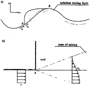
Figure 7: Application of the classical turbulent mixing layer model at the toe of the breaker
Despite these drawbacks, Cointe and Tulin [1] have applied the mixing layer model together with Bernoulli equation on the dividing streamline to define a relationship between breaker’s height and elevation of the breaking wave crest. Summing up their analysis, at the toe A of the breaker (Fig. 7a), the following relation holds
(6)
where vτ(A) is the flow velocity just downstream of A, while
(7)
is the flow velocity just upstream of A, being c the breaking wave propagation speed and y(A) the free-surface elevation over the undisturbed water level (y=0). Since the crest of the breaking wave is a stagnation point, it requires that ντ=0; hence, Bernoulli’s equation takes the form
(8)
where y(B) is the elevation of the crest of the breaking wave over the level y=0.
Equations (6) through (8) yield a simple relationship between the total height of the breaker [h*=y(B)−y(A)] and the elevation of the wave crest formulated as
(9)
This result (9) can be used for choosing a unique solution from a set of solutions calculated by means of the hydrostatic model of a spilling breaker and steady nonlinear potential theory provided β is evaluated on the basis of experimental data.
3 Steady breaking of periodic Stokes’ limiting waves
Breaking of sea waves in deep water may be related to growth of the wave amplitude due to wind or to interference with other waves. When the waves become steeper and reach some critical steepness, they may break with formation of spilling breakers. The steepest waves are known to be Stokes’ limiting waves with included angles of 120° at their crests. These waves are absolutely unstable and even a negligible disturbance of the flow could result in breaking of one wave. Therefore, the source of the disturbance of the waves may be omitted in the investigated problem so that the steady breaking phenomenon of Stokes’ limiting waves will be considered only.
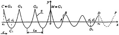
Figure 8: Breaking of Stokes’ limiting waves
With reference to Figure 8, the left-hand part of the free-surface flow consists of a semi-infinite train of incoming periodic Stokes’ limiting waves; one wave is broken and simulated by the flat-topped hydrostatic model of a spilling breaker; smooth waves of smaller amplitude follow downstream of the breaking wave. This steady problem is similar to the one considered by Tulin and Cointe [9] who utilized a linear wave theory and approximated the incoming waves of great amplitude by sin-shaped waves. Since this one is a too rough approximation for the problem at hand, in the new generalized approach the existence of actual Stokes’ limiting waves upstream of the breaking wave is assumed and a nonlinear potential method is introduced to simulate the free surface.
3.1 Problem statement
The steady and irrotational flow of an inviscid and incompressible fluid is considered. The free surface is fixed and flowed round by an uniform current with velocity c at infinity, which is equal to the propagation speed of the waves. Therefore, the governing equation for the velocity potential is
(10)
subject to the boundary conditions on the unknown free surface S
(11)
(12)
Equation (10) is the Laplace equation, equation (11) is the zero normal velocity boundary condition typical of steady flow, equation (12) is the Bernoulli equation modified by the presence of the breaker, S encompasses both the free surface and the surface SAB under the breaker, n is the outward unit normal vector on surface S, (x, y) is a Cartesian coordinate system which moves with the waves where axis y points vertically upwards from the undisturbed water level, Y is the ordinate of S, U=|∇Φ| is the velocity on S, with h=0 outside SAB and h>0 within SAB.
3.2 Numerical method
The unknown free-surface shape and the surface under the breaker, on which boundary conditions (11) and (12) should be fulfilled, are found through an iterative process of sequential approximations, thus updating the required shape of S step by step. An initial approximation So is set to define the shape of the free boundary S. On this surface, the velocity potential and, therefore, the velocity values are determined by the solution of the direct problem (10)–(11) in an area with known geometry. Verification of the modified constant pressure condition (12) is then produced and discrepancies are derived
at each point of the initial surface. If condition (12) is not fulfilled, a correction of the boundary is carried out, based on simplified equations of the inverse problem. Then, the updated surface shape is taken as the new trial one So, the velocity values on it are determined by the direct problem solution, check of the condition (12) is produced, and so forth, until this condition is satisfied. Summing up, every step of the iterative process consists of three main parts: i) solution of the direct problem (10)–(11) and definition of the velocity values on the boundary; ii) verification of the modified constant pressure condition (12); iii) solution of the inverse problem (correction of So).
The correction of the free boundary and of the surface under the breaker at every step of the iterative procedure is produced by means of quasi-linear equations. Despite the simplified character of the boundary shape correction, exact boundary conditions (11) and (12) are finally fulfilled. The accuracy of the whole problem solution depends on the accuracy of the direct problem (10)–(11) solution, which is the well-known Neumann boundary value problem. Simplifications introduced in the inverse problem compel to implement a procedure of sequential approximations. This procedure implies the development of a numerical technique for calculating cavitating flows of weightless fluid [18] and free-surface waves of finite amplitude [22].
3.2.1 Direct problem (velocity calculation)
A boundary integral method has been developed to calculate the velocity values on S at every step of the iterative procedure. A vortex layer is continuously distributed on a limited part CD of the infinite free surface as well as on the plate AB under the breaker (Fig. 8). Positive values are assigned to the required vortex intensity γ and to the angle between two directions, if they result in local counter-clockwise fluid rotation. Due to the periodic character of the waves in the far field both upstream and downstream, the wave trains are assumed to consist of waves whose shapes and velocity distributions on the free surface are similar to those of the edge semi-waves CC1 and D1D in the computational domain CC1M ABD1D.
Then a wide fictitious contour F1F2F3F4F5F6 is built (Fig. 9) in order to compile a Fredholm integral equation of the second kind for velocity calculation on S, which is similar to Melnikov equation for flows around foils [23]. The closed contour contains the calculation domain S identified by the path CC1M ABD1D, where mo and mf denote additional incoming and following waves, respectively, and by large horizontal rectilinear segments F1F2, F3F4 and F5F6 subject to the following constraints
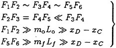
(13)
where Lo and Lf denote the length of the incoming and following waves, respectively. Since the contour F1F2F3F4F5F6 is closed, the velocity values U on it are equal to the intensity γ of the vortex layer
(14)
Equation (14) and constraints (13) allow to conclude that
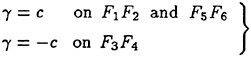
(15)
except on relatively small neighbourhoods of points F1, F2, F3, F4, F5 and F6.
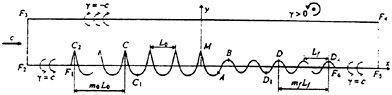
Figure 9: Scheme of fictitious closed contour
Then, the tangential velocity on S induced by the rectilinear segments of the closed contour, is considered. It is denoted by I with appropriate indexes related to the specific zone of the computational domain
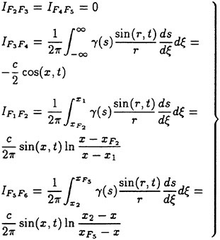
(16)
In the previous formulae x1 and x2 stand for the abscissae of points F1 and F6, x is the abscissa of any point on S where the velocity is calculated, t is the tangent to S in that point, r is the distance from a vortex to that point, s is the curvilinear abscissa measured on surface S. Finally, the joint induction from all rectilinear segments reads
(17)
Hence, the integral equation for calculating velocity values U on S can be formulated as
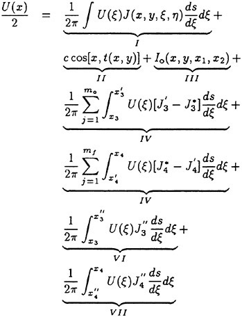
(18)
where
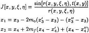
and
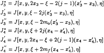
In equation (18) x and y denote the coordinates of any control point on S, while ξ and η represent the coordinates of the vortices on S. Abscissae ![]()
![]() are shown in Figure 8. The term on the left-hand side of equation (18) is the half-velocity at a control point within the integration domain [x3, x4]. The first term I in the right-hand side is the tangent velocity induced by vortices on [x3, x4]; the term II is the tangential component of the incoming flow; the term III is the tangent velocity—formula (17)—induced by the rectilinear segments of the fictitious closed contour; the term IV is the tangent velocity induced by γ distributed on the surface of mo imaginary periodic incoming waves copied from the edge semi-wave CC1; the term V is the similar velocity induced by γ on mf imaginary following waves; the terms VI and VII denote tangential velocities due to the last imaginary quarter-waves F1C2 and D2F6, respectively (Fig. 9). Integrals IV and V contain kernels composed by terms which correspond to the left- and right-hand imaginary periodic semi-waves, accordingly.
are shown in Figure 8. The term on the left-hand side of equation (18) is the half-velocity at a control point within the integration domain [x3, x4]. The first term I in the right-hand side is the tangent velocity induced by vortices on [x3, x4]; the term II is the tangential component of the incoming flow; the term III is the tangent velocity—formula (17)—induced by the rectilinear segments of the fictitious closed contour; the term IV is the tangent velocity induced by γ distributed on the surface of mo imaginary periodic incoming waves copied from the edge semi-wave CC1; the term V is the similar velocity induced by γ on mf imaginary following waves; the terms VI and VII denote tangential velocities due to the last imaginary quarter-waves F1C2 and D2F6, respectively (Fig. 9). Integrals IV and V contain kernels composed by terms which correspond to the left- and right-hand imaginary periodic semi-waves, accordingly.
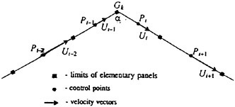
Figure 10: Flow modelling around the crest
The Fredholm integral equation of second kind (18) is solved numerically. Values of U, i.e. of the vortex intensity γ, are assumed to be constant on every rectilinear elementary panel on S. Control points are placed at the centres of the panels. Equation (18) is then reduced to a system of linear algebraic equations. At control points Pi, Pi+1 (Fig. 10) which are the nearest to the four crests of Stokes’ limiting waves Gk (k=1, 2, 3, 4) of the computational domain (Fig. 8), instead of equation (18) the following asymptotic formulae are used
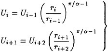
(19)
for potential flow inside the angle α enclosed by the tangents to the two branches of the wave at small neighbourhoods of the crest (α=2π/3). Here, velocities Ui and Ui+1 are calculated from values Ui−1 and Ui+2 at control points Pi−1 and Pi+2 which are the closest to Pi and Ρi+1, respectively; ri−1,
ri, ri+1 and ri+2 are the distances from the corresponding control points to the wave crest. Formulae (9) are introduced into the rows corresponding to points Pi and Pi+1 of the algebraic system, thus improving the accuracy of velocity calculation. The minimum sufficient number mo and mf of the additional periodic waves upstream and downstream of the calculation domain CD was determined by systematic calculations, which showed that values of U do not depend on mo and mf for mo=mf>10. Here mo=mf=20 has been assumed.
3.2.2 Inverse problem (surface correction)
In order to determine more and more correct shapes of the free surface S and to satisfy at each step of the iterative procedure all the conditions of the boundary value problem (10)–(12) from previous surface shape So, a correction of the trial surface will be produced through a quasi-linear approximation, i.e. assuming a small difference between the initial surface and the sought surface, which are smooth and have small curvature.
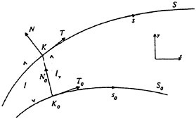
Figure 11: Notation for the inverse problem
The velocity potentials related to boundaries So and S are denoted as Φo and Φ, accordingly. The outward pointing unit normal and tangent vectors to these surfaces are no, to and n, t, respectively. It is assumed that the direct problem (10)–(11) has been solved for the initial surface So and that the potential Φo is known which satisfies the zero normal velocity condition
(20)
The distance l between two surfaces along direction no is considered as a variable which characterizes surface S with respect to the known surface So (Fig. 11). The potential function
(21)
is introduced to take into account the disturbance of the potential Φo caused by the deflection of the initial surface So and measured by distances l along no. Due to the small difference assumed between S and So, φ and l are small values too.
To compile equations of the inverse problem, it is necessary to denote the principal parameters of the surface S through the known parameters of the boundary So and the unknown functions φ(x, y) and l(so), where so is any abscissa measured along surface So. The normal and tangent vectors to the surfaces at corresponding points are bound together by the following relations
(22)
The derivatives of the potential Φ on S along n and t can be expressed through the derivatives of the potentials Φo and φ along directions no and to as
(23)
(24)
By using the Taylor-series expansion within a neighbourhood of size l around a point Ko on the surface So (Fig. 11), the values of the derivatives of the potentials Φo and φ on the surface S can be expressed through sums of the derivatives calculated on the known boundary So, in the form
(25)
(26)
(27)
(28)
By introducing expansions (25) through (28) into the derivatives (23) and (24) and then into the boundary conditions (11) and (12), and neglecting small terms of the second and higher order, a system of differential equations is obtained for the inverse problem as
(29)
where
(30)
is the velocity on the boundary So, yo denotes ordinates of So, ly is the projection of l on the vertical axis y. The former equation of the system (29) is the linearized representation of the zero normal velocity condition (11), whereas the latter is the linearized form of the modified constant pressure condition (12). The system (29) contains two unknown functions, that is, φ and l. After these functions are determined, ordinates Υ of the sought free surface S can be simply calculated as
(31)
The potential φ is represented by a continuous singularity distribution with strength σ on the initial boundary So
(32)
Since So is assumed to have a small curvature, equation (32) allows to write the first equation of the system (29) in the following form
(33)
By denoting the initial and ending point of the domain of So as a and b, respectively, and assuming the initial condition at the point a
(34)
the function l at whichever point so can be derived from equation (33) as
(35)
The increment of the tangential velocity on So caused by the presence of additional singularities on it, is represented by the singular integral
(36)
where sb is the abscissa of point b on So. By introducing formulae (35) and (36), the second equation of the system (29) can be transformed into the following singular integral equation for the unknown strength σ(so) of the singularities
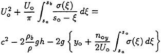
(37)
where noy is the projection of no on the vertical axis.
In the left-hand side equation (37) contains a Cauchy integral presenting a singularity at ξ=so. This equation may be solved by assuming a specific behaviour of the function σ(so) at the ends of the domain [sa, sb] and applying a desingularizing formula [24] for the Cauchy integral. Starting from the conditions σ(sa)=0 and σ(sb) → ∞, the trial free surface and surface SAB under the breaker are corrected accordingly, starting from the crest Μ of Stokes’ limiting wave which is the nearest to the breaking wave (Fig. 8). In practice, the point Μ is associated with the initial point a of the domain where the inverse problem should be solved. In the present modelling, the last point b is the crest Ρ of the third smooth wave downstream of the breaking wave (Fig. 8). Unlimited values of σ at this point do not cause any numerical difficulty because the last wave DP is cut off after the boundary correction. As a result, the following non-singular integral equation is introduced to correct the boundary at every step of the iterative procedure
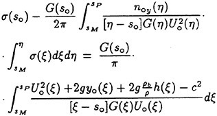
(38)
where ![]() being sM and sM the abscissae of the points Μ and P. Equation (38) is solved numerically by reducing it into a system of linear algebraic equations. Elementary panels and control points coincide with the ones selected in the direct problem, and intensity of singularitiess is assumed to be constant within any panel. After calculating the strength σ from equation (38), at each step the distances l from the corrected surface are obtained by formula (35). Finally, the ordinates of the free surface with breaker are determined by equation (31).
being sM and sM the abscissae of the points Μ and P. Equation (38) is solved numerically by reducing it into a system of linear algebraic equations. Elementary panels and control points coincide with the ones selected in the direct problem, and intensity of singularitiess is assumed to be constant within any panel. After calculating the strength σ from equation (38), at each step the distances l from the corrected surface are obtained by formula (35). Finally, the ordinates of the free surface with breaker are determined by equation (31).
3.3 Solution procedure
The left-hand side of the free-surface flow (Fig. 8) always consists of periodic Stokes’ limiting waves whose profiles are taken from previous results obtained by Amromin et al. [22]. When starting computation for a breaking solution, a trial shape of the right-hand side of the boundary with three smooth arbitrary waves and a flat-topped breaker on the front slope of the first wave are set. Then, velocity values are calculated from equation (18) at all control points of the trial boundary and used to verify the boundary condition (12). If the dynamic boundary condition is not satisfied with required accuracy, equation (38) is solved to obtain a new shape of the surface. The new position of the lowest point A of the breaker on the corrected boundary is automatically determined from the solution of the inverse problem, while the ending point Β of the breaker is not defined according to its previous position, but it is always placed at the wave crest. The step-by-step transformation of the breaker is depicted in Figure 12, where dotted lines and solid lines denote the free surface and the breaker before correction and after correction, respectively.
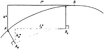
Figure 12: Transformation of the breaker
Thus, not only the free-surface shape, but also the dimensions of the breaker as well as the shape of the boundary beneath are updated during each step of the iterative procedure. The process is then repeated and the corrected surface is taken as a trial one at next step of iteration. Calculations terminate when the error in condition (12) becomes less than 2.5c2·10−5.
In practice, the most rational way of obtaining a set of solutions with different breakers was met in calculating a non-breaking shape of the free surface assuming h=0 everywhere, in placing a little breaker on the face of the first smooth wave and in deriving a breaking solution from this initial approximation. Later on, the front side of the breaker was slightly lowered with respect to the previous breaking solution. Calculations were then performed for the newly modified surface, and so forth, iterating for a solution.
4 Results and discussion
The fully nonlinear method developed in the previous section was applied to compute breaking of Stokes’ limiting waves. Two series of calculations were basically carried out; the former for nonbreaking smooth waves and the latter for breaking waves. The calculated breaking wave parameters have been compared with Duncan’s experimental results [2]. Accuracy of the numerical computations was verified by considering energetic balance between the incoming Stokes’ limiting waves, breaking wave and following waves.
4.1 Non-breaking solution
The calculated shape of a non-breaking free surface (Fig. 13) is composed of two semi-infinite trains, namely, Stokes’ limiting waves for x<0 and smooth periodic waves of high amplitude for x>0. The latter waves have a shape which is very close to the one for Stokes’ limiting waves except in the neighbourhood of the crests. The crest-to-trough height of these waves hf~1.32c2/(2g) is smaller than the height of Stokes’ limiting waves ho~1.49c2/(2g). It is obvious that waves with angled crest can not be obtained from computations unless one assumes their existence. Consequently, in order to improve accuracy when calculating the free surface in the neighbourhood of the crests, the following hypotheses were considered: i) the calculated smooth waves are analogous to Stokes’ limiting waves within the stated accuracy in numerical computations; ii) the height of the smooth waves and the surface curvature at the crests are increased until these waves
have a shape quite similar to Stokes’ limiting waves. The latter possibility is mainly dependent on dimensions of the local elementary panels. But these hypotheses have been found to be incorrect because the shape of the smooth waves is practically independent on the stated accuracy.
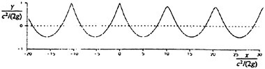
Figure 13: Non-breaking solution
Fortunately, the possibility of existence of the combined wave train can be explained from the wave energy point of view. Longuet-Higgins [25] discovered the remarkable fact that Stokes’ limiting waves do not have maximum energy parameters. In fact, according to formula (3) the value of Ro for Stokes’ limiting waves in deep water is about 0.01955ρc4/g, but a maximum value Ro=0.020ρc4/g was derived by Duncan [26] for smooth waves of a little, smaller steepness. Dependence of Ro on hoko, being ko the fundamental wave number, is as follows: Ro grows for hoko<0.82 and decreases for 0.82<hoko<0.87. Thus, there are smooth periodic waves with Ro value nearly equal to the one for Stokes’ limiting waves. Just these waves were calculated; their profiles are depicted in Figure 13.
4.2 Breaking solutions
A set of solutions was obtained assuming different sizes of the breaker and different amplitudes of the following waves downstream. Some examples of the free surfaces with flat-topped spilling breakers are shown in Figure 14.
In all calculations, the elevation YS of the breaking wave crest presented the same value, while the amplitudes Yf of the following waves over the undisturbed water level were practically constant at each test case in accordance with Duncan’s experimental data [2]. The limiting solution having the largest breaker and the smallest amplitude of the following waves is represented in Figure 14d.
The principal parameters of the calculated breaking waves versus normalized Yf are plotted in Figure 15, where h* and l* are the total height and length of the breaker, respectively, y(A) is the ordinate of the lower edge A of the breaker and the horizontal force Rb is calculated by means of formula (5). The larger the breaker, the smaller the amplitudes of the breaking wave and following waves; the lower the initial point A of the breaker, the higher Rb and hence the energy dissipation due to breaking.
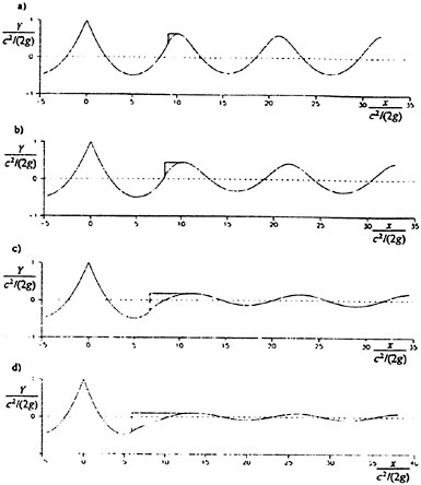
Figure 14: Breaking solutions
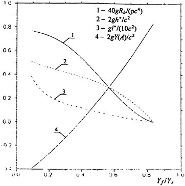
Figure 15: Principal parameters of breaking solutions
4.3 Comparison with experiments
Theoretical results have been compared with Duncan’s experimental data of breaking waves past a hydrofoil [2] in order to obtain a unique solution
which has to satisfy the criterion of existence of a stagnation point at the breaking wave crest in the case of viscous flow between the breaker and the underlying wave. To this purpose, calculated (solid curve) and experimental (squares) values of the total height h* of the breaker have been plotted versus the normalized elevation of the crests of the following waves (Fig. 16). Most of the experimental data are in good agreement with the theoretical results when introducing the value β2=0.5 into equation (9), except in the point representing the breaking onset. This regime means formation of a steep wave past a hydrofoil, which resembles Stokes’ limiting wave and rapidly breaks if a small disturbance is added to the flow. It corresponds to the value β2=0.41 in equation (9).
Obviously, breaking of free Stokes’ limiting waves differs from wave breaking past a hydrofoil. This fact is illustrated in Figure 16 where, in case of fully developed stages of breaking past a hydrofoil, significantly higher breakers take place with respect to the achieved numerical results. In any case, the regime of breaking onset is the most similar to breaking of Stokes’ limiting waves because the disturbances produced by a hydrofoil on the free surface are very low with respect to developed breaking stages.
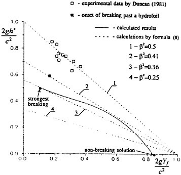
Figure 16: Total breaker’s height versus crest elevation of following waves
The computed strongest breaking solution turned out to be rather near to the experimental point of the breaking onset past a hydrofoil (Fig. 16). Moreover, for this solution formula (9) gives the value β2=0.36 which is the nearest to the value β2=0.25 corresponding to the classical mixing layer model. Therefore, it may be concluded that the numerically determined free-surface shape with the largest breaker more probably occurs under natural conditions.
4.4 Momentum flux
In the case of the strongest breaking solution numerical calculations yielded the values Rb=0.01910ρc4/g and Yf=0.08575ρc2/(2g). The wave breaking resistance can be used to evaluate the incoming wave momentum flux Ro of periodic Stokes’ limiting waves from the energy (resistance) point of view. Since the following waves have small amplitude with respect to their length, according to the linear theory it results
(39)
Inserting values of Rb and Rf into formula (3) yields the maximum wave resistance
(40)
in good agreement with Duncan’s calculations [26] which gave Ro=0.020ρc4/g for a wave with slope slightly smaller than Stokes’ limiting wave.
5 Concluding remarks
A generalized approach has been developed to investigate breaking waves with steady spilling breakers by substituting the area of breaking with a solid surface. This method is similar to application of cavity termination models and allows to reduce the problem into investigation of a steady potential free-surface flow. Consequently, complicated dissipative processes can be indirectly taken into account to evaluate wave breaking resistance as well as to estimate decreasing amplitudes of progressive waves after breaking.
Two simplified models for the breaking area have been considered, deriving that the hydrostatic flat-topped model of a spilling breaker is rather accurate and suitable for numerical computations. Insertion of this model into the newly developed nonlinear boundary integral method has allowed accurate numerical investigation of steady breaking of periodic Stokes’ limiting waves in deep water. A set of potential solutions with different breakers and wave
amplitudes has been obtained. It is noticeable that a non-breaking solution has been found consisting of Stokes’ limiting waves and smooth periodic waves (Fig. 14), thus confirming the possibility of its existence from the wave energy point of view. In accordance with Duncan’s observations [2] all breaking solutions have practically yielded equivalent crest elevation for the breaking wave and the same value of the crest elevation for the following waves downstream of a given breaker.
Comparison of theoretical results with experimental data has shown that the strongest breaking solution is the nearest to the breaking onset past a hydrofoil. Moreover, this solution is the most dissipative and gives a value of coefficient β which is the nearest to the classical turbulent mixing layer. Therefore, it is reasonable to assume that the strongest solution occurs in nature in accordance with the second thermodynamics law that states that nature prefers the most ‘dissipative solution.
Intermediate solutions with smaller breakers could be considered at sequential stages of the free-surface transition from a non-breaking condition into a final quasi-steady breaking condition. But this analysis would be a mere academic exercise since reliable experimental data regarding the transient phenomenon are still lacking, due to the fact that the breaker appears too rapidly during experiments.
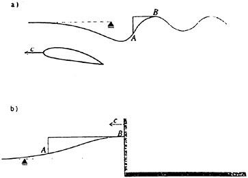
Figure 17: Further applications of hydrostatic model of a spilling breaker
Direct comparisons of achieved results with potential calculations by Tulin and Cointe [9] and Cointe and Tulin [1] were not carried out since they have approximated incoming waves by linear sin-shaped waves which have wave energy several times higher than Stokes’ limiting waves, so obtaining significantly larger breakers.
The hydrostatic model of a spilling breaker and the proposed numerical technique could be applied together also to investigate wave breaking past a hydrofoil (Fig. 17a) and in front of a blunt long body (Fig. 17b). In the first case, the experimental data [2], i.e. formula (9) with β2=0.5, should be used for choosing a unique solution from a series of feasible solutions, that is, for evaluating the balance between resistance due to wave breaking and the component due to the following waves. When investigating bow wave breaking, a unique solution will be automatically obtained since there should be no waves at infinity in front of the body.
Finally, it is authors’ opinion that in order to yield more accurate results when simulating free-surface flows with breaking waves, the hydrostatic model should be improved on the basis of new experimental data concerning the shape of a spilling breaker and the density of aerated water inside. In particular: i) the shape of the breaker should not be taken as flat-topped but parabolic, or should be defined by some more complicated affine function; ii) more exact value (even not constant along horizontal direction) of the water density in the breaker should be considered.
Acknowledgements
The present work was performed as a part of the scientific bilateral agreement between the Krylov Shipbuilding Research Institute and the Department of Naval Architecture, the University of Trieste. It has been developed during a 6 month post-doctoral study performed by the Russian author through a grant financed by the University of Trieste within the framework of the Italian law 19/1991 ‘Aree di Confine’. The Italian author is also pleased to acknowledge support provided by the Italian Ministry of Education under national contract MPI 40%.
References
[1] Cointe, R. and Tulin, M.P., “A Theory of Steady Breakers”, Journal of Fluid Mechanics, Vol. 276, 1994, pp. 1–20.
[2] Duncan, J.H., “An Experimental Investigation of Breaking Waves Produced by a Towed Hydrofoil”, Proceedings Royal Society London, Series A, Vol. 377, 1981, pp. 331–348.
[3] Mason, M.A., “Some Observations of Breaking Waves”, Gravity Waves, U.S. National Bureau
Standards, Circular No. 521, 1952, pp. 215–220.
[4] Longuet-Higgins, M.S. and Cokelet, E.D., “The Deformation of Steep Surface Waves on Water. II. Growth of Normal-Mode Instabilities”, Proceedings Royal Society London, Series A, Vol. 364, 1978, pp. 1–28.
[5] Peregrine, D.H., “Computations of Breaking Waves”, Preprint for NATO Advanced Research, Workshop on Water Wave Kinematics, 1989.
[6] Longuet-Higgins, M.S., “A Model of Flow Separation at a Free Surface”, Journal of Fluid Mechanics, Vol. 57, 1973, pp. 129–148.
[7] Banner; M.L. and Phillips, O.M., “On the Incipient of Breaking of Small Scale Waves”, Journal of Fluid Mechanics, Vol. 65, 1974, pp. 647–656.
[8] Longuet-Higgins, M.S. and Turner, J.S., “An Entraining Plume Model of a Spilling Breaker”, Journal of Fluid Mechanics, Vol. 63, 1974, pp. 1–20.
[9] Tulin, M.P. and Cointe, R., “A Theory of Spilling Breakers”, Proc. 16th Symposium on Naval Hydrodynamics, Berkeley, National Academy Press, 1986, pp. 93–105.
[10] Miyata, H., “Finite-Difference Simulation of Breaking Waves”, Journal of Computational Physics, Vol. 65, 1986, pp. 179–214.
[11] Mori, K. and Shin, M.S., “Sub-Breaking Waves: its Characteristics, Appearing Conditions and Numerical Simulation”, Proc. 17th Symposium on Naval Hydrodynamics, The Hague, National Academy Press, 1988, pp. 499–511.
[12] Lungu, A. and Mori, K., “A Study on Numerical Schemes for More Accurate and Efficient Comparison of Free-Surface Flows by Finite Difference Method”, Journal of the Society of Naval Architects of Japan, Vol. 173, 1993, pp. 9–17.
[13] Kawamura, T., Kawasima, H., Miyata, H. and Tsuchiya, Y., “CFD Simulation of the Flow around Craft and Tandem Hydrofoils”, Proc. FAST’95, Vol. 2, Lubeck-Travemünde, 1995, pp. 1181–1192.
[14] Trincas, G., “A Simulation Method for the Breaking Waves Generated by a Submerged Hydrofoil”, Proceedings of CMEM’97, Computational Mechanics Publications, Rhodes, 1997, pp. 533–542.
[15] Kang, K.J, “Numerical Simulations of Nonlinear Waves Generated by Submerged Bodies”, Post Doctoral Research Report, ISSN 1101–0614, Chalmers University of Technology, 1997.
[16] Sadovnikov, D.Y. “Application of Generalized Riaboushinsky Cavity Termination Model in the Problem of Gravity Wave Breaking”, Theses of Reports, XXXVI KSRI Conference, St. Petersburg, 1993, pp. 109–110 (in Russian).
[17] Sadovnikov, D.Y. “Gravity Nonlinear and Breaking Waves in Deep and Shallow Water”, Proceedings of the 1st International Shipbuilding Conference, Section B, St. Petersburg, 1994, pp. 190–197.
[18] Ivanov, A.N., “Hydrodynamics of Fully Cavitating Flows”, Sudostroienie, Leningrad, 1980 (in Russian).
[19] Dagan, G. and Tulin, M.P., “Two-Dimensional Free-Surface Gravity Flow past Blunt Bodies”, Journal of Fluid Mechanics, Vol. 51, 1972, pp. 29–43.
[20] Maklakov, D.V., “Analytical-Numerical Method for Calculating Nonlinear Waves past Ship Bottom”, Report of Kazanshky University, Kazan, 1992 (in Russian).
[21] Arie, M. and Rouse, H., “Experiments on Two-Dimensional Flow over a Normal Wall”, Journal of Fluid Mechanics, Vol. 1, 1956, pp. 129–141.
[22] Amromin, E., Ivanov A.N. and Sadovnikov, D.Y., “Bottom Effect on Limiting Stokes’ Waves”, Journal of Fluid Dynamics, Vol. 26, 1994, pp. 540–543.
[23] Melnikov, A.P., “About Vortex Method to Solve Problems of Flows Around Closed Contours”, LIIGVT, Vol. 4, 1936, (in Russian).
[24] Gakhov, F.D., “Boundary Value Problems”, Pergamon Press, Oxford, 1963.
[25] Longuet-Higgins, M.S., “Integral Properties of Periodic Gravity Waves of Finite Amplitude”, Proceedings Royal Society London, Series A, Vol. 342, 1975, pp. 157–174.
[26] Duncan, J.H., “A Note on the Evaluation of the Wave Resistance of Two-Dimensional Bodies from Measurements of the Downstream Wave Profile”, Journal of Ship Research, Vol. 27, No. 2, 1983, pp. 90–92.
Scattering of Internal Waves by a Circular Cylinder Submerged in a Stratified Fluid
N.Gavrilov, E.Ermanyuk, I.Sturova
(Lavrentyev Institute of Hydrodynamics, Russia)
ABSTRACT
The scattering of internal waves at circular cylinder submerged in continuously stratified fluid is studied theo retically and experimentally. The stratification is characterized by the presence of a layer of large density gradient (pycnocline) having finite thickness. The transmission coefficient for the incident internal wave of the first mode is obtained in relation to non-dimensional wave frequency and pycnocline thickness. It is experimentally shown that the scattering of internal waves is accompanied by non-linear effects. The transmitted wave train has a component with double frequency (second harmonic) compared to the incident wave frequency. The transmission coefficient of the second harmonic is measured.
The linear 2-D problem of internal wave scattering at a restricted cylinder is considered theoretically. The fluid is assumed to be nonviscous, incompressible and composed of three layers (the upper and lower layers are homogeneous and the middle layer is linearly stratified), which provides an approximate model of the experimental conditions. The Boussinesq approximation is used. The multipole expansion method is most efficient for solving the present problem, when a cylinder is fully immersed in the fluid layer of constant density. The comparison between theoretical and experimental data is presented.
INTRODUCTION
The sea wave propagation in the presence of different underwater obstacles and diffraction effect are the matters of great importance for marine engineering and underwater navigation. The problem of wave scattering by a submerged body has been investigated in detail for regular surface waves. However, for underwater objects placed near the region of high density gradient the study of internal wave scattering is the matter of considerable theoretical and practical interest.
The diffraction of surface waves on a submerged cylinder is a well-studied phenomenon. The absence of wave reflection at circular cylinder submerged in fluid of infinite depth has been shown by Dean [1]. In the fluid of finite depth the reflection is, in general, non-zero. However, zero reflection may be observed for a set of discrete wave lengths which are sometimes referred as bands of transparency (see, for example, Naftzger & Chakrabarti [2], Evans & Linton [3], Mallayachari & Sunder [4]). A study of internal wave diffraction at a circular cylinder in two-fluid system having free surface as the upper boundary and an interface between layers is presented by Linton & McIver [5]. It is shown that reflection is identically zero for a circular cylinder submerged in the lower layer of infinite depth. When the cylinder is submerged in the upper layer of finite depth, a certain portion of wave energy is reflected. Diffraction of internal waves at a submerged obstacle in continuously stratified fluid
has some specific features because each incident mode is scattered into an infinite number of modes. Numerical solution of 2-D linear diffraction problem for elliptic cylinder was obtained by Sturova [6] (two-layer fluid) and Gavrilov et al. [7] (three-layer fluid). The comparison between the experimental data and the computations presented in [7] reveals that the agreement between the predicted and measured loads is better for the horizontal component as compared to the vertical component what is especially notable at high wave frequencies. The approximate solution of diffraction problem for three-layer fluid is obtained by Sturova [8] under assumption that the body is immersed far from the middle layer.
The present report is organized as follows. The description of the experimental installation and technique is given in Section 2. The theoretical solution of the linear diffraction problem is presented in Section 3. Section 4 is dedicated to the analysis of numerical and experimental results.
2. EXPERIMENTS
The experiments were carried out in a test tank (4.5×0.2×0.6 m) filled with two layers of miscible fluids. The diagram of the experimental installation is shown in Fig. 1.
A weak solution of glycerine in water was used to create stratification. The fluid densities in upper and lower layers were ρ1=0.999g/cm3 and ρ2=1.0095g/cm3, respectively. The density distribution over depth ρ(y) may be well approximated by the following relation (the origin of the coordinate system is taken at free surface, the y-axis is directed upwards):
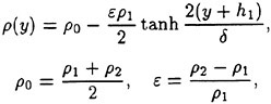
(1)
where h1 is the depth of the upper layer, δ is the characteristic thickness of the pycnocline. The depth of the lower layer is h2. The density distribution was measured by resistive probes. Since the diffusion coefficient of glycerine has low value,
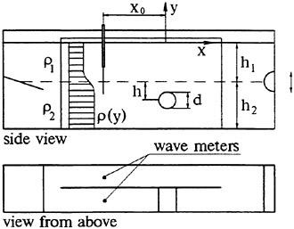
Fig. 1.
the variation of δ over one series of experiments was fairly small. The measurements taken prior to a series of experiments and after it demonstrated that the increase of δ did not exceed 0.2 cm.
The internal waves were generated by the wave maker undergoing harmonic vertical oscillations. The amplitude of oscillations A=0.6 cm, the frequency ω was varied. The test tank was equipped with a wave breaker. The wave breaker represented a flat plate inclined at 4° to the horizontal.
The experimental evaluation of reflection and transmission coefficients for surface waves at a submerged obstacle is normally based on comparison between the wave fields measured with and without an obstacle. Otherwise, one can use a method analogous to Grue [9]. According to this method one should formulate certain hypotheses about the structure of diffracted wave field. However, in the case of continuously stratified fluid the problem is complicated by complex modal structure of the diffracted wave field. Moreover, one should meet the necessary condition to reproduce all parameters of density distribution, in particular, the parameter δ. To attain these ends the test tank was partitioned by a thin longitudinal vertical plate in two identical channels of equal widths. A circular cylinder of diameter d=6 cm was installed in one of two channels. The distance between the centre of the cylinder and the middle of the pycnocline (ρ(y)=ρ0) is
denoted as h. The wave meters were installed in both parts of the test tank at equal distances from the wave maker. The horizontal distance between the wave meters and the axis of the submerged circular cylinder was x0=30 cm. The output of the wave meter installed at the lee side of the cylinder was treated as the characteristic of transmitted waves. The output of the other wave meter installed in the parallel channel was treated as the characteristic of the incident wave. The cylinder was located at the distance 170 cm from the wave maker.
The operation principle of the wave meters is based on the measurement of conductivity of medium between two closely-spaced vertical wires. The output of the wave meters e is related with density distribution ρ(y) as follows:
where e0 and e1 are dimensional constants, y1 and y2 are vertical coordinates of the lower and the upper ends of wires. If the vertical displacements of fluid particles η(y) are small, the time-dependent component of the output signal ![]() may be written
may be written
where f(t) is a harmonic function of time, the prime denotes differentiation with respect to y. In experiments the length of wires met the condition (y2−y1)>2δ, so that the following relations were satisfied with high accuracy: ρ(y1)=ρ1; ρ(y2)=ρ2; ρ′(y1)=ρ′(y2)=0. To perform a static calibration, the wave meters were vertically displaced by a known distance in otherwise quiescent fluid. Thus, a resistive wave meter with vertical wires records the following measure of internal wave intensity:
(2)
This value is the weighted (with ρ'(y) as the weight function) mean value of the amplitudes of vertical displacements of fluid particles in pycnocline. Let us note that for a sharp density variation (free surface or an interface) the derivative ρ'(y) is Dirac delta-function. In this case the definition of ![]() according to (2) reduces to usual definition of amplitude.
according to (2) reduces to usual definition of amplitude.
In experiments the wave maker generated the internal waves of the first internal mode. The measure of intensity of these waves defined by (2) is denoted as η0. It should be noted, that the experimental value of η0 was small (η0<0.15 cm).
The scattering of incident internal waves is accompanied by the excitation of high internal modes. Moreover, in certain range of parameters non-linear effects manifest themselves in the excitation of the second harmonic at the lee side of a submerged obstacle. The spectral analysis of the output signal of the wave-meter placed at the lee side of the submerged circular cylinder allowed to evaluate the intensities of the first and the second harmonics which are denoted as η1 and η2, respectively.
The value η1/η0 characterizes the ratio between the intensities of transmitted and incident waves. This value is, in a limited sense, analogous to the usual definition of the transmission coefficient. However, one should keep in mind the important difference introduced by the integral in (2). It is easy to see that the main contribution to the value ![]() is produced by the internal modes having uneven numbers, the input due to each particular mode being difficult to isolate. Nevertheless, the value η1/η0 represents an important measure which reflects the most important features of the wave scattering.
is produced by the internal modes having uneven numbers, the input due to each particular mode being difficult to isolate. Nevertheless, the value η1/η0 represents an important measure which reflects the most important features of the wave scattering.
In experiments the parameters of internal waves of the first mode satisfied with high accuracy the following dispersion relation [10]
(3)
where k=2π/λ is the wave number of the first internal mode.
3. THEORETICAL ANALYSIS
It is assumed that the inviscid incompressible fluid occupies the region −∞<x<∞, −Η<y<0 and there are three layers: homogeneous
upper and lower ones and a linearly stratified middle one. Thus, density stratification in an undisturbed state ρ(y) takes the form
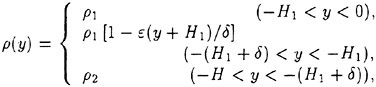
where H1=h1−δ/2 is the depth of upper layer, Η=h1+h2 is the total depth of the fluid. This three-layer fluid is the model of a smooth pycnocline and approximates the density distribution (1). Let us transfer the origin of the coordinates to the lower boundary of the middle layer by the translation ![]() .
.
We investigate the scattering of an internal wave of the given mode, incident on a solid horizontal circular cylinder which is fully immersed in the lower layer. The assumption that the cylinder is positioned outside of the pycnocline is crucial. To our knowledge, the problem for a body which intersects the pycnocline or is placed inside it has not yet been analysed even within the linear approach.
The cylinder axis is parallel to the front of the incident wave, so that the problem considered is 2-D one. it is assumed that the upper layer is bounded by a rigid lid. The disturbed oscillating motion of the fluid is assumed to be steady and the flow inside upper and lower layers is potential.
In the upper and lower homogeneous layers the total velocity potentials ![]() satisfy the equations
satisfy the equations
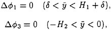
where H2=H−H1−δ is the depth of lower layer.
The internal wave equations for the vertical velocity ![]() in the middle layer are written within the Boussinesq approximation
in the middle layer are written within the Boussinesq approximation
where ![]() is the buoyancy frequency or Brunt—Vaisala frequency. In the general case
is the buoyancy frequency or Brunt—Vaisala frequency. In the general case ![]() . The boundary conditions are the following
. The boundary conditions are the following
(4)
(5)
(6)
(7)
It is known from the theory of linear internal waves that in such a fluid the existence of free internal waves is possible only with ω<Ν. The wave incident from the right can be an arbitrary internal mode with a vertical velocity
(8)
The wave number k satisfies the dispersion relation
(9)
where μ=kχ, ![]() t1=tanh kH1, t2=tanh kH2. There exists a countable number of values kj(k1<k2<…), satisfying the given dispersion relation. The eigenfunctions
t1=tanh kH1, t2=tanh kH2. There exists a countable number of values kj(k1<k2<…), satisfying the given dispersion relation. The eigenfunctions ![]() for the vertical velocity of the wave modes are represented in the form
for the vertical velocity of the wave modes are represented in the form
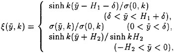
where
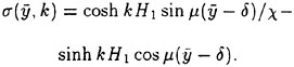
The eigenfunctions are orthogonal
(10)
The vertical velocity of the incident wave in (8) is conveniently expressed by
where
By analogy with Sect. 2 let us define the amplitude of internal wave as the average value of the vertical displacements of fluid particles over the thickness of a middle layer. The vertical displacement of fluid particle ![]() is determined from ∂η/∂t=υ0. In this case η0 is the dimensional value of incoming wave amplitude.
is determined from ∂η/∂t=υ0. In this case η0 is the dimensional value of incoming wave amplitude.
The total velocity potential in the lower layer can be written as
Here the incident wave potential ![]() of the l-th internal mode has the form
of the l-th internal mode has the form
and we seek the diffraction potential as
The boundary condition at cylinder surface S: ![]() has the form
has the form
(11)
where a=d/2 is the radius of the cylinder, ![]() is the distance from the centre of the cylinder to the lower boundary of middle layer,
is the distance from the centre of the cylinder to the lower boundary of middle layer, ![]() is the inward normal to the cylinder surface. In addition, the radiation condition must be satisfied, implying that only waves outgoing from the body are generated due to the scattering.
is the inward normal to the cylinder surface. In addition, the radiation condition must be satisfied, implying that only waves outgoing from the body are generated due to the scattering.
We can find the solution of this problem by the multipole expansion method. This method was used by many authors for the solution of different radiation and diffraction problems (see, for example, the list of references in [5]).
To write the solution in terms of the multipole expansion, we define the polar coordinates
The multipole expansion for the diffraction potential ![]() in the upper layer may be written as
in the upper layer may be written as
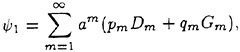
(12)
where
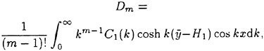
(13)
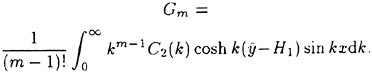
(14)
The potential ![]() in the lower layer is
in the lower layer is
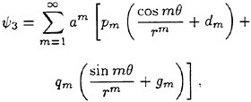
(15)
where
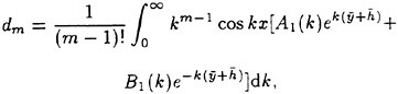
(16)
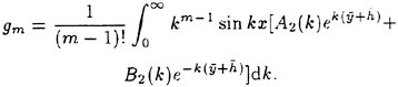
(17)
The vertical velocity of the scattering wave in the middle layer is
The multipole expansion for ![]() is
is
(18)
where
(19)
(20)
Using the relation
and the boundary conditions (4)–(7), we can determine the functions A1,2(k), B1,2(k), C1,2(k), X1,2(k), Y1,2(k). For example, the relations for A1,2(k) and B1,2(k) have the form
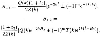
where
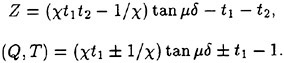
At ω<Ν the integrands in (12)–(20) have a countable number of the simple poles kj (j=1, 2,…) which represent the roots of the equation Z(kj)=0. This is tantamount to the dispersion relation (9).
Using the radiation relation, equations (16)–(17) then become
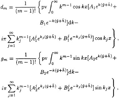
where the symbol pυ indicates the principal value integration and the superscript j denotes the residue of corresponding function in the point k=kj.
To impose the body surface condition, we use known relations
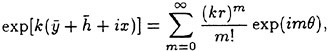
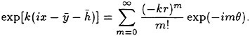
Equation (15) then becomes
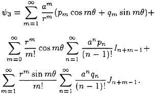
(21)
where
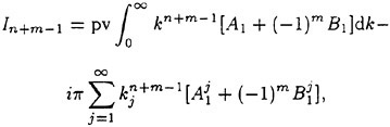
(22)
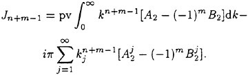
(23)
Differentiating (21) with respect to r and using (11), we obtain the systems of linear equations for determining of pm and qm
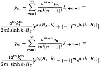
The solution of these equations may be obtained by truncating the infinite series at a finite number of terms, which depends on the desired accuracy.
One of the concerns in the diffraction problem is the exciting forces ![]() . They can be computed from
. They can be computed from
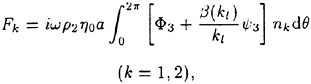
where
and are equal to
In far field (x → ±∞) the diffraction potential in the lower layer is
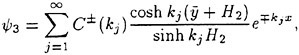
(24)
where C±(k)=T2(k)±T1(k),
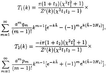
As the result of solution of the diffraction problem, we can determine backward (x → ∞) and forward (x → −∞) scattering matrices ![]() where for each element the row number l corresponds to the incident mode number, and the column number m—to the number of scattered internal wave mode. The wave scattering parameters are conveniently determined with use of energy evaluation (10)
where for each element the row number l corresponds to the incident mode number, and the column number m—to the number of scattered internal wave mode. The wave scattering parameters are conveniently determined with use of energy evaluation (10)
The complex values ![]() and
and ![]() are the transmission and reflection coefficients of the l-th internal mode, respectively. For the deep lower layer the backward scattering waves are absent because pm=−iqm at H2 → ∞ and hence
are the transmission and reflection coefficients of the l-th internal mode, respectively. For the deep lower layer the backward scattering waves are absent because pm=−iqm at H2 → ∞ and hence ![]()
![]() for exciting forces F2=−iF1. The approximate values of these functions are obtained in [8] for the body located in the deep lower layer far from the middle layer.
for exciting forces F2=−iF1. The approximate values of these functions are obtained in [8] for the body located in the deep lower layer far from the middle layer.
4. RESULTS AND DISCUSSION
When obtaining the multipole expansion solution the high accuracy can be achieved by using only several terms in (12), (15), (18). The following numerical results are obtained by using five terms what implies an error less than 10−3. The numerical integration is performed with relative error 10−4. On this basis the number of terms in the infinite sums (22), (23) is determined.
In the considered problem it is of interest to investigate the influence of pycnocline thickness on the loads acting on the cylinder. In an undisturbed state the mean line of pycnocline is located on fixed depth h1=a, the total depth of fluid is equal to Η=5a, the distance from the centre of cylinder to the mean line of pycnocline is equal to h=2a, relative difference of density between lower and upper layers is ε=0.03. The incident wave is the first mode (l=1).
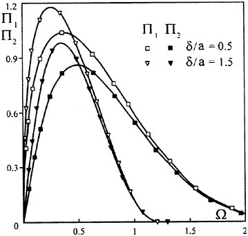
Fig. 2.
The numerical results for non-dimensional exciting forces Πj=|Fj|(2+ε)/ρ2η0aεg depending on Ω=aω2(2+ε)/εg are shown in Fig. 2. The light and dark squares correspond to the pycnocline thickness δ/a=0.5 (H1/a=0.75, H2/a=3.75,), ![]() the light and dark triangles correspond to δ/a=1.5 (H1/a=0.25, H2/a=
the light and dark triangles correspond to δ/a=1.5 (H1/a=0.25, H2/a=
![]() ). The light (dark) squares and triangles represent the results for the horizontal Π1 (vertical Π2) exciting forces. The value ω=Ν corresponds to Ω=3.94(1.31) at δ/a=0.5(1.5).
). The light (dark) squares and triangles represent the results for the horizontal Π1 (vertical Π2) exciting forces. The value ω=Ν corresponds to Ω=3.94(1.31) at δ/a=0.5(1.5).
As the thickness of pycnocline increases the maximal values of exciting forces also increase. But at fixed wave frequency for Ω>0.7, the greater pycnocline thickness corresponds to shorter incident internal wave, with a consequent drop of diffraction loads.
In the case being considered the thickness of the lower layer is relatively small and the horizontal exciting forces are greater than the vertical exciting forces.
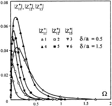
Fig. 3.
The backward scattering coefficients are presented in Fig. 3. The input parameters of Fig. 3 and Fig. 2 are the same. The curves 1–3 (4–6) correspond to the reflection coefficient ![]() the scattering coefficients of the first mode in the second
the scattering coefficients of the first mode in the second ![]() and in the third
and in the third ![]() ones at δ/a=0.5 (1.5), respectively. From Fig. 3 we notice that the amplitude of scattered waves increase with increased thickness of pycnocline.
ones at δ/a=0.5 (1.5), respectively. From Fig. 3 we notice that the amplitude of scattered waves increase with increased thickness of pycnocline.
In the first series of experiments the cylinder was entirely placed in the fluid layer of constant density ρ2, i.e. the density variation over the range of depth within the limits h±a was vanish
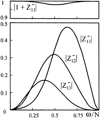
Fig. 4.
ingly small what complies with the assumptions adopted in theoretical formulation of the problem.
The comparison of the theoretical and experimental results is performed at H1=12.85 cm, δ=4.3 cm, H2=27.85 cm, ![]() ε=0.01051. The absolute values of the transmission coefficient
ε=0.01051. The absolute values of the transmission coefficient ![]() and the forward scattering waves
and the forward scattering waves ![]() for the first three modes are shown in Fig. 4. The transmission coefficient is just slightly different from 1 despite the fact that the forward scattering wave
for the first three modes are shown in Fig. 4. The transmission coefficient is just slightly different from 1 despite the fact that the forward scattering wave ![]() is pronounced.
is pronounced.
As different internal modes of given frequency ω have different wavelengths, the inputs in the signal of the wave meter due to each particular mode may be either summed up or subtracted from each other depending on their phase shifts in the point of measurements. Referring to Eq. (24), the output of the wave meters depends not only on the frequency of the incident wave but also on their spatial position. Shown in Fig. 5 are the results of calculations for x0/d=5, 15, 25. The numerical results are compared with experimental data for x0/d=5. As is seen from Fig. 5. the experimental and numerical data agree quite
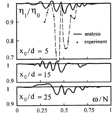
Fig. 5.
well qualitatively. At the same time there is a notable quantitative disagreement. This disagreement may be explained by the effects of viscosity and by the presence of discontinuity of the density gradient in the three-layer system.
In the second series of experiments the cylinder was partially submerged in the pycnocline. In this case the cylinder reflects a part of wave energy. The smaller is h/d, the greater is the portion of reflected wave energy and the lower is the value η1/η0. This effect is illustrated in Fig. 6 by the data obtained at h1/d=2.5, h2/d=5 for the following set of parameters: curve 1−h/d=1, δ/d=0.58; curve 2−h/d=0.75, δ/d=0.54; curve 3−h/d=0.6, δ/d=0.58. It easy to see that the effect is most pronounced for the incident waves of small length. The pycnocline plays the role of a waveguide and the cylinder represents an obstacle in this waveguide. The same effect is observed when the submergence of the cylinder is held fixed while the pycnocline thickness increases. The value k is related with frequency ω by Eq. (3) which was experimentally proven. It should be noted that for the experimentally studied range of parameters the dispersion relation for the first internal mode (3) agrees well with the complete dispersion relation (9).
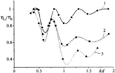
Fig. 6.
The non-linear effects accompanying the diffraction of waves at a submerged obstacle manifest themselves by the emergence of high-frequency components of wave field at the lee-side of an obstacle. Normally, the second harmonic having doubled frequency compared to the frequency of the incident waves is most pronounced. Under suitable conditions the amplitude of the second harmonic may be equal to the amplitude of the first harmonic [9].
The non-linear effects accompanying the diffraction of internal waves in continuously stratified fluid have not yet been studied in detail. Some qualitative descriptions of the observed wave patterns are given by Gavrilov & Ermanyuk [11]. In continuously stratified fluids the frequency range of high-order effects is limited by the value ω=Nm/2, where Nm is the maximum value of Brunt-Vaisala frequency N(y). The internal waves of second harmonic can not be excited when the frequency of incoming waves ω>Nm/2. It is interesting to determine the frequency range corresponding to most pronounced non-linear effects.
The results of experiments are shown in Fig. 7 for h1/d=2.5, h2/d=5, h/d=0.75: curves 1. 2 represent η2/η0; curves 3, 4—η1/η0; curves 5, 6—η0/d. Dark and light symbols correspond to δ/d=0.42 and δ/d=0.55, respectively. For surface waves of sufficiently small amplitude the value η2/η0 is directly proportional to η0/d [9]. The similar dependence should be expected for
internal waves. In experiments the amplitude η0 and the steepness parameter kη0 of the incident waves were small and varied within a narrow range. Thus, the dependence η2/η0 on ω/Nm shown in Fig. 7 gives a clear notion of the frequency range within which the second harmonic is markedly excited. As seen from the Fig. 7, the maximum values of η2/η0 measured at different δ/d take place at the common value ω/Nm≈0.34 while the corresponding non-dimensional lengths of the incident waves are different (kd=0.68 at δ/d=0.42 and kd=0.52 at δ/d=0.55). Using the dispersion relation (3) one can evaluate that under experimental conditions the energy transferred to the second harmonic did not exceed 1.4% of the incident wave energy. However, the presence of the second harmonic at the lee side of the submerged cylinder led to approximately three-fold increase of the local slopes of the curves ρ(y)=const in the middle of the pycnocline compared to the slopes in the incident wave system.
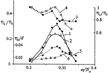
Fig. 7.
Thus, the perturbations of the local parameters of the diffracted wave field due to non-linear effects may be considerable. On the other hand, the non-linear mechanism of the energy transfer from low to high frequencies due to interaction of internal waves with complicated bottom topography may be of considerable interest on a large scale.
CONCLUSIONS
The present study continues the investigations started by the authors in [7]. It is experimentally shown that diffraction of internal waves at the circular cylinder is attended with the effects conditioned by complex modal structure of internal wave field. The characteristics of scattered waves essentially depend on position of the cylinder with respect to pycnocline. The portion of wave energy reflected by the cylinder drastically increases as the cylinder approaches the middle of pycnocline.
In the case of a cylinder located outside of the pycnocline the theoretical solution of linear diffraction problem is obtained by multipole expansion method. The theoretical solution clarifies a number of qualitative effects observed in experiments. The present results may be useful for the estimation of the accuracy of the numerical algorithms used for a body of an arbitrary form. An effective numerical method of the solution of the linear diffraction problem for a body submerged outside of the pycnocline is the coupled finite-element method (CFEM). This method was applied to study the diffraction of internal waves by a submerged elliptic cylinder in [7]. The comparison of the numerical results obtained for a circular cylinder in a three-layer fluid by CFEM and the solution given in the present report showed fair agreement.
In future, the multipole expansion method with point multipoles can be used to study the diffraction of internal waves at a submerged sphere.
The reason for quantitative disagreement between theory and experiments necessitates further investigations. To describe the observed nonlinear effects manifested by the emergence of high-frequency components of wave field, high order theory should be developed.
ACKNOWLEDGMENT
This work was supported in part by the Siberian Division of Russian Academy of Sciences (SD RAS) under the integrate grant no. 43.
REFERENCES
1. Dean, W.R., “On the Reflection of Surface Waves from a Submerged, Circular Cylinder,” Proceedings of the Cambridge Philosophical Society, Vol. 44, 1948, pp. 483–491.
2. Naftzger, R.A., and Chakrabarti, S.K., “Scattering of Waves by Two-Dimensional Circular Obstacles in Finite Water Depth,” Journal of Ship Research, Vol. 23, No. 1, 1979, pp. 32–42.
3. Evans, D.V., and Linton, C.M., “Active Devices for the Reduction of Wave Intensity,” Applied Ocean Research, Vol. 11, 1989, pp. 26–32.
4. Mallayachari, V., and Sunder, V., “Wave Transformation over Submerged Obstacles in Finite Water Depths,” Journal of Coastal Research, Vol. 12, No. 2, 1996, pp. 477–483.
5. Linton, C.M., and McIver, M., “The Interaction of Waves with Horizontal Cylinders in Two-Layer Fluids,” Journal of Fluid Mechanics, Vol. 304, 1995, pp. 213–229.
6. Sturova, I.V., “Plane Problem of Hydrodynamic Rocking of a Body Submerged in a Two-Layer Fluid without Forward Speed,” Fluid Dynamics, Vol. 29, No. 3, 1994, pp. 414–423.
7. Gavrilov, N., Ermanyuk, E., and Sturova, I., “The Forces Exerted by Internal Waves on a Restrained Body Submerged in a Stratified Fluid,” Preprints of 21st Symposium on Naval Hydrodynamics, Trondheim, Norway, 1996, pp. 254–265.
8. Sturova, I.V., “Effect of Anomalous Dispersion Dependencies on Scattering and Generation of Internal Waves,” Journal of Applied Mechanics and Technical Physics, Vol. 35, No. 3, 1994, pp. 366–372.
9. Grue, J., “Nonlinear Water Waves at a Submerged Obstacle or Bottom Topography,” Journal of Fluid Mechanics, Vol. 244, 1992, pp. 455–476.
10. Phillips, O.M., The Dynamics of the Upper Ocean., 2nd ed., Cambridge Univ. Press, Cambridge e.a., 1977.
11. Gavrilov, N.V., and Ermanyuk, E.V., “Effect of a Pycnocline on Forces Exerted by Internal Waves on a Stationary Cylinder,” Journal of Applied Mechanics and Technical Physics, Vol. 37, No. 6, 1996, pp. 825–831.
DISCUSSION
J.Grue
University of Oslo, Norway
The paper describes an interesting study on the interaction between internal waves and a submerged cylinder. Main focus is paid to transmission and reflection properties of the waves. The paper combines theoretical modeling and experiments, which is useful. In the theoretical part the linear diffraction problem in a three-layer fluid due to the presence of a cylinder in the lower layer is solved. Results for the wave field are presented. In addition, the induced forces are calculated in a few examples. The experimental part of the study is both as interesting as it is complex. Interesting linear and nonlinear features of the wave field are reported. I think that the authors could have spent more space to describe experimental results which I believe are available.
Both theory and experiments are carried out with thicknesses of the pycnocline, leading to results that describe a broader picture. It would, however, also be interesting if results for an infinitely thin pycnocline (δ/α=0) could be included in figures 2 and 3, for comparison. In view of the force computations in figure 2, did you also in the experiments measure the induced forces?
The comparison between the wave computations and the wave measurements is quite good in some cases, but less good in other cases. The disagreement between the two approaches is attributed to the effect of viscosity and a discontinuous density gradient in the three-layer system. I wonder if it is possible to calibrate a set of experiments that fit with the assumptions of the theory, where an eventual disagreement between the two approaches can be reduced to a minimum, at least for some parameters?
The results on the second harmonic waves are interesting. I wonder if observations in nature of this phenomenon exist?
AUTHORS’ REPLY
In the present experiments the measurement of forces has not been conducted. However, in the Proceedings of the 21st SNH (see reference [7] of our paper) the authors have presented the results of experimental investigation of loads acting on a submerged elliptical cylinder due to internal waves in stratified fluid having pycnocline. It is the authors’ belief that the qualitative physical effects for the circular cylinder are the same, although some quantitative difference must be expected.
In more detail the theoretical results are presented by Sturova [1]. Among other things the results for an infinitely thin pycnocline are included.
In the authors’ opinion it is possible to make special calibration or some refinement of experimental technique which can allow a fit with theoretical approach. It seems promising to conduct the measurements of the scattered internal wave field by the wave gauge translated horizontally at small constant speed. In this case the inputs due to different modes (having the same physical frequency but different wavelengths) will be separated due to Doppler effect and, as a result, be easily detectable by Fourier analysis. The analysis of inputs due to isolated modes seems to be easier and a better fit with the present theoretical approach based on presentation of internal waves as a sum of different modes.
The generation of internal waves of second harmonic was reported in the oceanographic literature in relation to tidal currents. It was observed that tidal oscillations of stratified fluid in the presence of an underwater mountain can generate internal waves having doubled frequency compared to the frequency of tidal motion.
Reference
1. Sturova, I.V., “Diffraction and Radiation Problems for the Circular Cylinder in Stratified Fluid,” (submitted to Fluid Dynamics).
DISCUSSION
C.M.Linton
Loughborough University, United Kingdom
Over the past five years or so problems associated with wave diffraction in stratified fluids have received considerable attention.
There have been three different types of approach—numerical, analytical and experimental—and all three have a role to play in increasing our understanding in this area.
Gavrilov et al.’s paper presents both experimental and analytical work, but in this discussion I will restrict my comments to the analytical part of the paper. As far as I am aware this work represents the first analytical attempt to solve an internal wave diffraction problem in which the interface between the two layers of fluid of different density is modeled by a layer of finite thickness in which the density gradient is large (a so-called pycnocline). This is incorporated into a two-dimensional model in which both the upper and lower layers have finite thickness and are bounded by a rigid wall.
The authors have analyzed wave scattering for this fluid configuration using the method of multipoles which typically allows problems in which the scatterer is a horizontal cylinder to be solved efficiently and accurately. This is what Gavrilov et al. have done and they confirm that only a small number of terms are required in the multipole expansions to achieve accurate results. The results which are presented are both useful and interesting, particularly those which show the effect of varying the thickness of the pycnocline on the hydrodynamic characteristics. Multipoles for two finite fluid layers separated by a sharp interface and bounded by rigid walls were first derived by S.E.Kassem (Math. Proc. Camb. Phil. Soc. (1982) 91, 323–329), and the derivation of the multipoles in the present paper represents an extension of Kassem’s work to the case of a finite pycnocline.
In the experiments that are described, the upper boundary of the upper layer is not a rigid wall but a free surface and the effect of changing this boundary condition in the theoretical analysis is not discussed. It would be interesting to know if the authors have any quantitative estimates of the effect of this approximation. In Linton & McIver (1995) (cited) multipoles were used to examine
scattering problems which contain both a free surface and a sharp interface, in which case energy can be transferred between internal and free surface waves. Presumably a similar analysis could be performed for the finite pycnocline situation and this would have an effect on the calculated results which may bring the experimental and theoretical results closer together.
Another aspect of Linton and McIver’s work was the systematic derivation, from Green’s theorem, of identities connecting the various hydrodynamic quantities which arise, such as reflection and transmission coefficients and exciting forces, and which are analogous to those that exist in standard linear water-wave theory. Presumably similar results exist for a finite pycnocline, both with the free surface approximated by a rigid lid and with the linear free-surface boundary condition applied. Such relations are of intrinsic theoretical importance and can also be used as a check on results obtained from any numerical procedure.
AUTHORS’ REPLY
We agree that the theoretical analysis can be performed with consideration the free surface on the upper boundary. Effect of the free surface on scattering of the internal waves in the two-layer fluid was studied by Sturova [1]. In the experiments described in the present paper the density variation over depth was very small what implies that the transfer of energy from internal modes to surface motion at free surface has been observed in experiments.
Indeed, the identities connecting the various hydrodynamic quantities exist for a finite pycnocline and are obtained by Sturova [2].
References
1. Sturova, I.V., “Scattering of Surface and Internal Waves on Submerged Body,” Computational technology, Vol. 2, No. 4, ICT SD RAS, Novosibirsk, 1993, pp. 30–45 (in Russian).
2. Sturova, I.V., “Diffraction and Radiation Problems for the Circular Cylinder in Stratified Fluid,” (submitted to Fluid Dynamics).


