
A Perspective on Naval Hydrodynamic Flow Simulations
A.Arabshahi, M.Beddhu, W.Briley, J.Chen, A.Gaither, K.Gaither, J.Janus, M.Jiang, D.Marcum, J.McGinley, R.Pankajakshan, M.Remotigue, C.Sheng, K.Sreenivas, L.Taylor, D.Whitfield (Mississippi State University, USA)
ABSTRACT
A perspective of computational hydrodynamics is presented that is considered relevant to particular Naval hydrodynamic problems. This is not intended as a survey of the field in general; rather, it is a summary of the ongoing research and development of computational tools in the Computational Fluid Dynamics Lab at Mississippi State University. A discussion is given of the enabling technologies on which most of the computational tools are based. Example results are presented for submarines, surface ships, and propulsors, that attempt to illustrate the current status of certain Naval hydrodynamic computational capabilities. Some observations and comments are offered relating to various needs and possible directions of future computational hydrodynamic research and development.
1.0 INTRODUCTION
This invited paper deals primarily with the development and application of Reynolds Averaged Navier-Stokes (RANS) codes to Naval hydrodynamic problems. The paper discusses some of the computational tools being developed in the CFD Lab that can be brought to bare on these hydrodynamic problems, and it also attempts to address some interesting but difficult underlying questions related to an assessment of present and future computational fluid dynamics (CFD) capabilities and requirements.
Recent increases in computer speed have not reduced typical runtimes for complex or advanced simulations, primarily because decreases in computer memory cost have increased the memory available, which in turn has made it possible to obtain numerical solutions to larger and far more complicated problems. The emergence of parallel computing is providing large global memory and runtimes which are reduced by multiple processors, and this is also enabling the solution of larger and even more complicated problems. Three-dimensional computations are now being performed rather routinely. In many cases, these computations have been and are being performed for either isolated components of complicated configurations or for steady state flows, and usually for both. Parallelization is now making it possible to obtain some reasonable measure of turnaround time for complete configurations in which all components are accounted for in their true interaction mode, and in some cases this is being done for both steady and unsteady flow situations. The complexity of flow configurations that are feasible will continue to increase, and along with this will come the need to address widely-varying time and length scales in the same physical problem. This, in turn, will invite further advances in both solution methodology, computer hardware and computational software.
The present paper is not intended as a survey of CFD for Naval hydrodynamics. Rather, it is primarily a summary of ongoing research in the CFD Laboratory of the NSF Engineering Research Center at Mississippi State University and through its associations with other agencies within the Navy, NASA, and Air Force. Some of the enabling technologies that have contributed to the development of certain hydrodynamic tools are first briefly reviewed in Section 2. Example results are then presented in Section 3 for simulations related to submarines, surface ships, and propulsors. Section 4 then offers some observations and comments relative to an assessment and suggested direction of CFD for Naval hydrodynamics. This section should be considered for no more than what it is, namely the opinions of the authors. Some conclusions are drawn in Section 5.
2.0 ENABLING TECHNOLOGIES
This section reviews briefly the technologies that form the basis for the tools used for the computational hydrodynamics results presented in the following
section. The topics covered are the usual grid generation and flow solver summaries, followed by the approach used for the dynamic relative motion grid computations required by rotating propellers. Following these are brief discussions on parallelization, graphics, and lastly, some comments relative to a CFS (Computational Field Simulation) system that is being developed to aid in code utilization and technology transfer.
2.1 Grid Generation
Structured multiblock grids have been used for some time for the computation of steady and unsteady Naval hydrodynamic problems. However, unstructured grid technology has been an active area of research, and the fruits of this effort are now beginning to be used for these same hydrodynamic problems. Consequently, both structured and unstructured grid generation capabilities are summarized.
2.11 Structured Multiblock
The structured grid generation code is a General Unstructured Multi-Block (GUM-B) structured grid generation system that evolved from the research and development of the structured grid technology within the NGP system [1]–[5]. Unstructured Multi-Block pertains to the issue of partial face matching, and the emphasis is that the block faces can be composed of multiple interfaces or subregions that can be interconnected to other block faces. Through the use of the solid-modeling data structure, the block connectivity is explicitly defined, so user intervention is not required to indicate block interfaces and orientations [2] [3]. Grid information of shared elements is automatically distributed to the adjoining parts [2] [4], thus allowing the user the freedom to concentrate on the domain decomposition.
The foundation of GUM-B has evolved to software reusability. The graphical user interface (GUI), Geometry/CAD, and graphics are now supported via independent libraries which are utilized by other research and educational efforts at the Engineering Research Center. The GUI was redesigned to be more intuitive and easy-to-read, and it was developed by an in-house package called GuiDe [6]. GuiDe provides easy-to-use GUI design and editing, prototyping of C code, and a convenient library of widget functions and links into the graphics server. The graphics server libraries have been developed on the Open Inventor object-oriented toolkit [7] [8]. The graphics server library was developed to take advantage of the available toolkit features, but is flexible enough to replace the underlying graphics, independent of GUM-B. The Geometry/CAD functions of NGP [1] [4] [5] were also packaged into a reusable library, allowing the underlying geometry engine to be replaceable within GUM-B, but usable for other systems.
2.12 Unstructured Grid Generation
Marcum and Weatherill [9] developed a very efficient local-reconnection procedure using advancing-front point placement and a combined Delaunay/min-max (minimize the maximum angle) type local-reconnection for generation of triangular or tetrahedral element grids. This approach is known as AFLR (Advancing-Front/Local-Reconnection). It differs substantially from earlier methods in that the combined Delaunay/min-max reconnection criterion is the only criteria developed to date which allows effective optimization of a three-dimensional tetrahedral element connectivity, by making effective use of the existing grid as a search data structure. Point insertion is performed using direct subdivision of the elements that contain them. This methodology has also been extended for generation of high-aspect-ratio elements [10], right-angle elements [11], and solution-adapted grids [12].
An advancing-normal type point placement strategy is used for the generation of high-aspect-ratio elements. The local-reconnection procedure, in conjunction with the advancing-normal point placement procedure does produce sliver elements in three dimensions. These elements are generated only in regions of high-aspect-ratio elements with a very structured alignment. A modified process that does not produce sliver elements is used for three-dimensional cases. The element connectivity is generated along new points in high-aspect-ratio regions. Local-reconnection is not used to determine the connectivity in these regions. This procedure produces a very structured connectivity and allows the tetrahedral elements to be easily combined into structured type elements. Typically, the majority of the tetrahedral elements within the high-aspect-ratio region can be combined into six-node pentahedrons (prisms). The outer layer of this region may have some five-node pentahedrons (pyramids) to match the outer tetrahedral elements. In all cases, the pentahedral elements have strict node, edge and face matching to each other and to neighboring tetrahedral elements.
High-quality grids have been generated about geometrically complex configuration using this procedure. Results verify that for isotropic grid generation, advancing-front point placement with a combined Delaunay/min-max connectivity criterion consistently produce the highest element quality in an efficient manner [13].
2.2 Flow Solvers
The discussion above of the structured and unstructured grid generation technology used is followed here by a brief discussion of both the structured and unstructured flow solvers.
2.21 Structured Multiblock
The numerical approach is to solve the three-dimensional time-dependent incompressible turbulent Navier-Stokes equations. These equations are first transformed to a time-dependent curvilinear coordinate system. The artificial compressibility idea of Chorin [14] is then introduced [15]–[17]. The use of artificial compressibility permits the experience gained in the numerical solution of compressible flow problems to be exploited in the numerical solution of incompressible flow problems [18]. The artificial compressibility form of the three-dimensional time-dependent Navier-Stokes equation in general curvilinear coordinates is
(1)
where
In these equations, β is the artificial compressibility coefficient, with a typical value of 5~10; p is static pressure; u, v, and w are the velocity components in Cartesian coordinates x, y, and z. U, V, and W are the contravariant velocity components in curvilinear coordinate directions ξ, η, and ζ, respectively. Terms ![]() where k=ξ, η, and ζ, are the viscous flux components in curvilinear coordinates. J is the Jacobian of the inverse transformation, and kx, ky, kz, and kt with k=ξ, η, and ζ are the transformation metric quantities [17], where a subscript denotes differentiation.
where k=ξ, η, and ζ, are the viscous flux components in curvilinear coordinates. J is the Jacobian of the inverse transformation, and kx, ky, kz, and kt with k=ξ, η, and ζ are the transformation metric quantities [17], where a subscript denotes differentiation.
In this work, the thin-layer approximation is introduced to simplify the full Navier-Stokes equations. An algebraic turbulence model [19], a k-ε model, and a nonlinear k-ε model [20] have been implemented within the code and used for the turbulent flow computations. The details of treating the viscous terms are explained in the work of Gatlin [21]. In addition, improvements have been made by Chen [22] with regard to the computation of the wall shear stress by improving the computation of the tangential velocity derivatives normal to a solid surface. This improvement is simple to implement and works extremely well on grids that may be highly skewed [22].
Equation (1) is discretized into a cell-centered finite-volume form. The cell face numerical flux vector was obtained using the flux difference split scheme of Roe [23]. The nonlimited form of the dependent variable extrapolation method of Anderson, Thomas, and van Leer was used to obtain second and third-order flux vectors [24]–[27]. The numerical flux used for the results presented here is the third-order upwind-biased scheme [27].
The normal procedure for the solution of the discretized equations would be to linearize the spatial difference terms, move the terms not containing ΔQn to the right-hand side of the equations, and solve for ΔQn [28]. This is particularly true for problems expected to have steady state solutions because the sum of the spatial difference operator terms as well as ΔQn would both go to zero. However, for unsteady flow, the ideal situation would be to find Qn+1 such that, for one dimension
(2)
One way of attempting to solve this problem is to use Newton’s method. Newton’s method [29] for the function ![]() would be
would be
(3)
where m=1, 2, 3,… and ![]() is the Jacobian matrix of the vector
is the Jacobian matrix of the vector ![]() . In principle the generated sequence Qn+1,m+1 converges to Qn+1 and, hence, Eq. (2) is satisfied.
. In principle the generated sequence Qn+1,m+1 converges to Qn+1 and, hence, Eq. (2) is satisfied.
A linear system of equations must be solved at each iteration of Newton’s method. For three-dimensional problems a direct solution seems to be impractical [30] and in this work symmetric Gauss-Seidel relaxation is used. Because the flux Jacobian of the flux vector based on Roe’s formulation is difficult to obtain analytically in three dimensions, and also in the interest of simplicity, the flux Jacobian is obtained numerically [30] [31]. The solution scheme is referred to as discretized Newton-relaxation [29], or the DNR scheme [30]. Multigrid is used to accelerate the numerical solutions [32]. This multigrid scheme has been extended to multiblock [33] and unsteady flow
[34]. The solution process is, therefore, a multigrid scheme for three-dimensional unsteady viscous flow on dynamic relative-motion multiblock grids.
The basic flow solver, called UNCLE (UN-steady Computation of fieLd Equations), has been modified for free-surface capability. The important difference between free-surface flows and other kinds of flows is that one has to obtain the motion of the free surface as part of the solution. One uses the kinematic condition [35], [36] to track the motion and the dynamic boundary conditions [37] (together with the continuity equation) to obtain the velocity and pressure at the free surface. Since the problem involves the motion (deformation) of one of the fluid boundaries, the governing equations can be cast either with respect to an inertial frame or with respect to a non-inertial frame. In the UNCLE solver the non-inertial frame is used which means that the free surface is always represented by a constant curvilinear coordinate surface. This approach involves grid motion and regeneration of the grid below the free surface at every instant in time. The basic UNCLE solver has been extended to handle difficult free surface problems such as the wetted transom flow behind the DTMB 5415 model, incorporating all the above mentioned changes.
2.22 Unstructured Solver
An efficient unstructured flow solver is being developed for simulations of three-dimensional unsteady compressible and incompressible high Reynolds number viscous flows about complete configurations. Clearly, achieving this goal is not easy, and requires that several limiting barriers be overcome. Firstly, the computational cost is one of the most pressing hurdles for performing large-scale simulations about a complete configuration. This computational cost is associated with the inherently large amount of memory required by unstructured solvers, and the relatively large CPU time required. Secondly, until very recently [38] there has been limited success at generating three-dimensional unstructured high-aspect ratio elements for realistic simulations of complex geometries in extremely large Reynolds-number flows. These fundamental issues must first be resolved in order for the unstructured approach to be useful in real-world applications of complete configurations.
An efficient unstructured flow solver for three-dimensional compressible and incompressible turbulent flows is being developed and further advanced. The basic solution algorithm is that of Anderson, Rausch, and Bonhaus [39]. It solves the three-dimensional Reynolds averaged Navier-Stokes equations, with the artificial compressibility formulation for incompressible flow. The Spalart and Allmaras [40] one-equation turbulence model is used to model turbulence. The discretized scheme uses a node-based finite-volume upwind approximation. The numerical flux for the inviscid part is evaluated using a second-order Roe scheme, while the viscous flux is evaluated with a finite-volume formulation that is equivalent to a Galerkin type of approximation. The time-advancement algorithm is based on the linearized backward Euler time-difference scheme, which yields a linear system of equations for the solution at each time step. The Gauss-Seidel procedure is used to solve the linear system of equations at each time step. The current work introduces an effective multiblock strategy [41] and mixed-element method to significantly reduce the memory requirements and computational time. Multigrid acceleration, dynamic moving grid capabilities, and parallelization will be added to the solver to further improve the efficiency and to predict the trajectory of unsteady maneuvering vehicles by coupling the unstructured solver with the 6-DOF solver.
2.3 Dynamic Relative Motion Grid Computations
The method used to include an actual rotating propulsor is one that has been continually developed and used for a number of years, primarily for compressible flows [42]–[47]. The approach is to use relative motion blocks with structured grids, whereby the blocks that include the rotating blades move relative to adjacent blocks with a region of the blocks near the relative motion interface being treated using the localized grid distortion technique introduced by Janus [43]. This method of handling relative-motion blocks insures the continuity of grid lines (although they do change partners periodically, or “click”) and restricts the maximum distortion of the grid to be of the order of the distance between grid points, which is of course small for viscous grids. This approach eliminates the need to interpolate the solution vector from one grid to another. The cell volumes do change in time, however, and the geometric conservation law must be satisfied [48].
2.4 Transition to Scalable Parallel Computing for Complex Simulations
The computer resources required for large-scale complex flow simulations are very substantial. Parallel computing can reduce the calendar time for running large cases by at least two or three orders of magnitude, and can provide access to the large global memory required for many larger problems. Consequently, portable scalable parallel implementations of the solution methodology are needed to enable the practical solution of large-scale problems and problems with long-term transient evolutions.
Parallel solution algorithms have been developed and implemented in a parallel code that enables a validated transition from single-processor computations to scalable parallel solution on complex large-scale practical applications. The parallel code exploits
coarse/medium-grained parallelism using the Single Program Multiple Data (SPMD) model, and employs MPI for message passing in view of its extensive portability and functionality. Much of the validation was accomplished by re-running cases that had provided validation for single-processor versions of the code.
The parallel code solves the three-dimensional incompressible unsteady RANS equations using an implicit finite-volume approximation in multiblock transformed coordinates, with characteristic-based upwind flux approximations. The implicit approximation is solved at each time-step using a Multigrid/Newton/Relaxation procedure analogous to that used in the sequential algorithm [31] [34]. Domain decomposition is used to partition and map the data space onto a set of processors. Static load balancing is done at the grid generation stage when possible, based on a heuristic performance estimator which takes into account the characteristics of the algorithm and the available system resources [49]. The time-linearized approximations at each time-step are solved using a block Jacobi symmetric Gauss-Seidel relaxation procedure that involves a point-to-point message exchange at each sub-iteration level. The code also uses point-to-point messages to handle the rotating interface required for handling propulsor calculations. The implementation of algebraic turbulence models includes user-defined collective operations over processor subsets.
The parallel code has been used extensively for simulations of isolated propulsors and for various submarine geometries involving hull, sail, sail planes, stern appendages, propeller, and moving control surfaces. For example, solutions for a fully-configured submarine with rotating propeller using a 1.6 million-point grid have been obtained using 51 processors on an IBM-SP (thin nodes). The parallel runtime is 57 minutes (1.5 Gflops) for one propulsor revolution of 160 time-steps, whereas the sequential solver requires 32 hours per propulsor revolution on an IBM 590 workstation.
Other examples have been run on a Cray T3E: A 4.5 million-point solution for a P5168 propeller with two-equation turbulence model requires 18.8 hours (42 processors) for the 1500 steps needed for a steady solution. An 11 million-point solution for the 11:6 count Sirenian propulsor requires 50 hours (87 processors) for five revolutions (5000 steps). A 4.5 million-point solution for a full-configuration SUBOFF geometry with k-ε turbulence model requires 7 hours (64 processors) per propeller revolution (300 steps).
The parallel solutions typically have efficiencies (percent CPU utilization) of 80–95 percent. Sealability studies using heuristic performance estimates indicate that on current-generation hardware, parallel efficiencies of 80 percent and more can be achieved on up to 400 processors and 50 million points, using appropriately-sized grids.
2.5 Graphics
Visualization of computed data presents several problems. First is the issue of the data itself. Current trends and technologies enable the solution of problems which produce enormous amounts of data. Often, a great deal of the post-processing time is spent just sifting through, culling out, and extracting data from files too large to read into the limited memory on a graphics workstation. Another issue is that of how to visualize the data. One often does not know a priori what features exist and which are important in the solution data. Consequently, much time is spent “stumbling” through the data in an effort to locate these features. This is especially true in data sets involving complex geometries and complex physics. Other problems exist due to the often cumbersome nature of many of the currently-available visualization software systems and to the constantlychanging state of the art.
To address these problems, the people who perform the post processing and visualization tasks at the ERC work and communicate closely with those who perform the computational simulations. Several commercially-available software packages are currently used for post processing of CFD data, these including PLOT-3D, FAST, and PV3. Emerging technologies are continually sought and evaluated as to their capabilities and usefulness. Another software system called DIVA (Data Interactive Visualization and Analysis) [50] is under development at the ERC. DIVA is built upon graphics server and user interface libraries designed to be portable, reusable, and maintainable. The development of this software has been driven primarily by the visualization needs of the computational engineers.
2.6 CFS System
Computing a computational field simulation (CFS) solution involves a number of steps, including components of geometry, grid generation, field simulation solvers, and visualization. Each of of these steps has traditionally been completed using a separate program. To facilitate a technology transfer vehicle that permits the creation of domain-specific problem solving environments for various field simulation applications, an integrated modular environment is being developed that provides a single and unified graphical user interface (GUI) to the software elements needed to compute a CFS solution. This environment is referred to as the CFS system.
The software development goal is to build highly cohesive (all modules of a library are self-contained), loosely coupled (a module does not depend on modules outside its respective library) reusable software libraries with well defined application programmer interfaces (APIs) between the libraries. This approach reduces the amount of software maintenance, speeds up the development of new systems, and reduces errors.
The APIs isolate the application developer in one library from changes in another library. By using the reusable-library model, a number of grid generation and visualization subsystem components, including SolidMesh (unstructured grid generator), GUM-B (structured grid generator), and DIVA (solution visualization) have been incorporated into the CFS system.
Graphics and the user interface are the issues of most concern when considering portability between computer platforms. The graphics server API abstracts the application programmer from a specific graphics language. OpenInventor has been used as the primary graphics language for the graphics server due to its portability across multiple platforms, including UNIX workstations and PCs. All user-interface activities are handled through the GuiDe API and are implemented in X Windows/Motif.
3.0 EXAMPLE NUMERICAL RESULTS
A few example numerical results are presented and discussed in this section. These results are for submarines, surface ships, and propulsors. The submarine results include a rotating propeller, so in this context, the body and propulsor are coupled in their natural interaction mode, including crashback. However, there will also be a few results given on an isolated propulsor because there is a good set of experimental data with which to compare.
3.1 Submarines
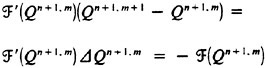
The submarine configuration considered here is the so-called SUBOFF geometry [51]. Numerous comparisons have been made with this configuration over the past few years. There are various appended configurations that include the bare hull, the bare hull with four stern appendages, and the bare hull with the sail. All of these configurations were considered in [52]. Numerous solutions at several angles of drift were computed and compared to experimental data in [52] [33] using the Baldwin-Lomax turbulence model. The results of this exercise resulted in extremely good agreement with experimental data, much better than one might expect, even to 18 degrees of drift. An example of this agreement is given in Figure 1 where the axial, normal, and pitching moment coefficients are compared with experimental data for the SUBOFF bare hull with four stern appendages.
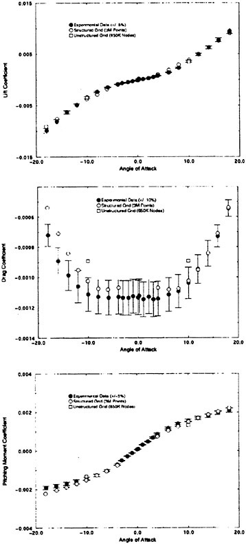
Figure 1. Numerical and Experimental Data Comparisons for the SUBOFF Body with Four Stern Appendages
Figure 2. Unstructured Viscous Grid in Stern Region of SUBOFF Configuration
Most of the numerical solutions in Figure 1 were carried out on a structured grid. However, one unstructured grid solution was obtained for 10 degrees angle of attack and the results are included in Figure 1. The unstructured grid used for this computation had 850,000 nodes for the complete configuration, whereas, the structured grid had 1.5×10⁶ grid points for half the body. The stern region of the unstructured grid is shown in Figure 2.
A more compelete configuration was constructed by adding a sail plane and rotating propeller to the basic SUBOFF geometry. The configuration then consisted of the hull, sail, sail plane, four stern appendages, and a rotating propeller. A visualization of the solution for this fully-configured geometry is shown in Figure 3. Maneuvering predictions were obtained for this configuration by combining the Navier-Stokes solver and a 6-DOF solver [53]. The first maneuvering prediction was carried out by Dreyer at ARL/Penn State [54] with a body-force propulsor in place of the rotating propeller. Subsequent to this calculation, a maneuvering prediction solution for a fully-configured geometry that included the actual rotating propeller in place of the body-force propulsor, was carried out by Davoudzadeh [55]. This maneuver included crashback. This computation was obtained by letting the body move roughly at cruise speed, which was determined from the coupled Navier-Stokes and 6-DOF solutions, and then the propeller rotation was decreased from the constant-rpm forward rotation speed, through zero, and up to a constant-rpm reverse rotation. The results of this maneuver are recorded in [55]. A propeller in crashback creates a vortex ring around the propeller as shown in Figure 4. The strength of this vortex ring depends on such things as the rotation rate of the prop and the velocity of the boat. The ring is not stable and unsteady side forces are created. Examples of the strength and orientation of this vortex ring are shown in [55].
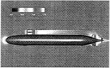
Figure 3. Axial Velocity About the Full SUBOFF Configuration at 0° Angle of Attack
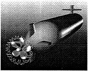
Figure 4. Vortex Ring Produced by the Crashback Maneuver
3.2 Surface Ships
A submarine in crashback is a difficult computation. However, a surface ship with a wetted transom stern flow is also a most difficult computation. The numerical solution of Model 5415 at a Froude number of 0.2756 is one such solution. The solution for the wave profile on the hull for this Froude number at a Reynolds number based on body length of 12.02 million is shown in Figure 5. The computed particle traces on the free surface in the transom stern region are also shown in Figure 5. The computed vortex, which can be seen in the enlarged view of the stern region, is in agreement with experimental measurements by Toby Ratcliff of DTMB [56]. The computed resistance at this Froude number and Reynolds number differs from Ratcliff’s experimental data by 1.2%. Details of this computation and additional comparisons with experimental data are given in [57].
There is considerable amount of experimental data available for the Wigley hull and the Series 60 hull. Both of these configurations have been computed and computational details and comparisons with experimental data for the Wigley hull form is given in [58], and the same for the Series 60 hull form are given in [59].
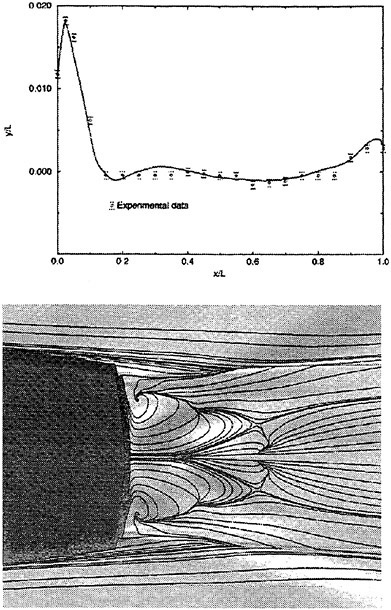
Figure 5. Numerical and Experimental Results for Model 5415 at Fr=0.2756
3.3 Propulsors
Where propulsors are included in their natural interactive mode, such as on a submarine configuration, the computations are carried out in the absolute frame. The SUBOFF results with the rotating propeller were obtained in this manner. Another example where this approach was used is the ΜIT notional geometry, known as Sirenian, designed by Kerwin [60]. This geometry had 11 inlet guide vanes, or stators, and 6 rotating blades, in other words, a non-even blade count stage propulsor. The grid had about 11 million points and an example of the grid for the propulsor region is shown in Figure 6. This propulsor is attached to a full body; therefore, the natural interaction of the propulsor with the hull boundary layer is taken into account. This solution was run using the parallel version of the UNCLE code and the grid consisted of 87 blocks. No experimental data exists for this configuration; however, the numerical results shown in Figure 7 for flow through this two blade-row propulsor seem plausible.
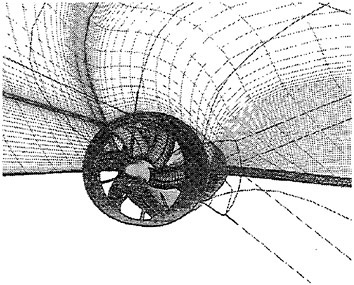
Figure 6. Structured Grid About the 11:6 Blade Count Sirenian Configuration
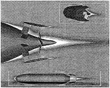
Figure 7. Numerical Solution of the Sirenian Configuration
For isolated propellers, considerable CPU time and memory can be saved by using a relative-frame version of the propeller code. Numerous propeller solutions have been obtained using this approach and the results have been compared to experimental data where available. However, there is a particularly detail set of experimental measurements that were taken by Jessup [61] on propeller P5168 at the David Taylor Model Basin. The purpose of these experiments was to investigate the propeller blade-tip vortex. An example of the axial, radial, and tangential velocity components just downstream of the propeller is given in Figure 8 for an advance ratio of 1.1. Numerous grid sizes were investigated in these computations that included structured multiblock grid densities of 300,000 to 1,500,000 points. Also various turbulence models were investigated that included algebraic, two-equation linear models, and two-equation non-linear models. For these computations the non-linear models gave essentially the same result as the linear two-equation models. There was a difference, of course, among the different solutions as indicated by the line plots in Figure 8. However, the overall agreement between the numerical and exper-
imental results for essentially all the turbulence models and grid densities considered, was consider good. The numerical results in the shaded plots in Figure 8 used the fine grid Baldwin-Lomax algebraic turbulence model.
4.0 OBSERVATIONS AND COMMENTS
The organizing committee asked that certain questions be addressed in this paper. Among these questions are: (1) what are the limitations of RANS codes and how well do they approximate the physics of real flows, (2) how well do the various turbulence models approximate the physics of flows, and for what type of flows of interest are the various turbulence models applicable, (3) how does grid selection influence the solution, (4) how does one check on uncertainty in the calculation, (5) have RANS codes been pushed as far as they can be and what future research needs to be done for development of RANS codes, and (6) what will be the new tools for the future? The authors do not feel qualified, capable, nor comfortable in attempting to answer these questions in a definitive way. However, something will be said about each topic, in no particular order, if for no other purpose than to stimulate thinking in those that may be capable of answering these questions.
4.1 An Application-Oriented Perspective on Flow Simulations and Turbulence Models
The resolution needed for flow simulations (number of points and local distributions) is affected by both geometric and physical factors. The geometry introduces its own length scales and resolution requirements. For example, a submarine geometry typically has elements such as a hull, sail, sail/bow planes, stern appendages, propulsor, control surfaces and gaps, and corner regions near adjoining surfaces.
Although the physical flow structure varies widely from problem to problem, external flow problems often have a uniform free stream (potential flow) with shear-layer development (laminar, transitional or turbulent) near solid surfaces. These surface layers require local resolution and also have important influences on the remaining flow structure. Vorticity generated on surfaces is transported by convection and diffusion, and the surface shear layers may themselves separate, detach or lift off of the surface, transporting vorticity and turbulence well away from the surface. This in turn generates new flow structures requiring local resolution, including vortices and wakes.
If a surface layer is turbulent, then turbulent correlations or shear stresses arising from time averaging (RANS) or space averaging (LES) exert an important local influence on the flow. Once a surface layer detaches, the vorticity transported into the flow can manifest itself as regions of rotational inviscid flow in which turbulence itself (if present) may have negligible
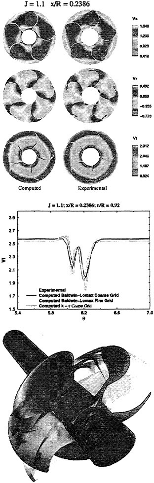
Figure 8. Numerical and Experimental Data Comparisons for Propeller P5168
influence on the flow behavior in an averaged sense, so that much of the flow is locally governed by the rotational inviscid Euler equations, even though the source of the vorticity is surface layers with turbulence. This can easily occur in three-dimensional flows, in which inviscid secondary flows are generated by turning a primary flow that has nonzero transverse vorticity. There is often strong physical interaction between the surface layers and the rotational inviscid regions, but the turbulence itself may be important only in very limited regions such as the surface layers and may not need to be modeled very accurately in much of the flow. If detached flow structures are present in which the turbulent shear stresses are not negligible, then they would require adequate modeling, provided they exert an important influence in the particular application of interest. In the authors experience, different implementations of specific turbulence models have given poor predictions by introducing too much modeled turbulence in what are essentially rotational inviscid regions resolvable by high-resolution flow solvers. The effects of turbulent transition are much more subtle and can be influenced or triggered by turbulence outside the wall layer which itself exerts negligible shear stress.
The point of all this is that flow applications with turbulence are physically complicated, and the importance and difficulty of modeling turbulence and validating turbulence models may depend on the particular application domain. Thus, it is dangerous to generalize about the validity of turbulence models, and the lack of a generally valid universal turbulence model may not prevent substantial affordable progress in a given application domain.
4.2 Implications for Flow Solvers, Equation Sets and Turbulence Modeling
To summarize some of these comments, although turbulence plays an important role in establishing the (averaged) flow structure to be resolved, much of the flow resolution requirements and computational cost for practical flow simulations can come from complex inviscid flow structures induced by geometry and wall layers. Since it is only recently becoming possible to obtain high resolution simulations for unsteady three-dimensional flows, the authors believe there is still much to be learned about the sources of error in specific applications of interest, whether from numerical, turbulence modeling, or experimental sources. Although systematic studies of error, uncertainty, verification and validation of flow simulation codes will continue to be needed, the effective use of flow simulation for complex applications is not becoming a routine exercise. Although the simulation code itself need not require a developer/specialist to use, it should be used by a specialist in simulations for the given application category.
Since the interaction between localized turbulence and larger inviscid flow structures can be very complex and application dependent, and since the cost of proving grid independence for a complex unsteady three-dimensional simulation is very high, it will probably remain difficult for some time to distinguish numerical, experimental and turbulence-modeling errors in a general problem independent way. For cases in which the turbulence modeling is important in localized regions, it may be that refinements to existing RANS turbulence models, although not universally valid, can provide very effective tools in specific problem domains, when used appropriately.
Recent increases in computing power, coupled with concerns about the lack of universality and predictive accuracy of RANS turbulence models have led to interest in Large Eddy Simulation (LES) methods for future simulations. The unsteady RANS equations are time-averaged over a time scale sufficient to average turbulent fluctuations into Reynolds stresses, while leaving the larger scale rotational inviscid motions to be resolved as unsteady phenomena. The LES equations employ a spatial averaging over a scale sufficient to filter scales not resolved by the particular grid being used, and the subgrid scale turbulence is then modeled. The unsteady RANS and LES approaches are very similar with regard to the solution algorithm, code development and validation needed, and both require some form of turbulence model that can be incorporated in modular form.
The primary difference is in the degree of mesh resolution required, since LES resolves the larger eddies of the turbulence itself, whereas the unsteady RANS approach models the turbulence and resolves the unsteady structures larger than the turbulent eddies. Consequently, LES typically requires much higher grid resolution, at least locally, and is therefore more costly. On the other hand, LES only models the subgrid turbulence structures and is universally applicable to the extent that a universal grid-independent subgrid model can be established. Since the unsteady RANS and LES codes can presumably be implemented in modular form as alternative turbulence or subgrid models, they are on equal footing in regard to the need for efficient and accurate unsteady flow solvers, and validation studies.
4.3 Influence of Grid Selection
In most practical simulations, solutions change in some degree when the grid is changed. The manner and degree of grid dependence is expected to depend on the problem, the flow solver, grid generation capabilities, and what is of particular interest in the solution. For example, the near-wall grid spacing required to resolve a turbulent boundary layer seems to depend on many things. Some approaches may require much finer resolution than others, and the spacing required to obtain an accurate numerical flux near a wall may be so small that the solver used cannot handle the numerical stiffness. On the other hand, the solver may be adequate for the
small mesh spacings, but the flux formulation used may require a very small spacing. Confronted with this, the developer may find the use of wall functions attractive, but, this approach still has it’s own requirements for grid resolution. Again, it is difficult at this time to generalize about quantitative grid requirements, and experience with individual flow solvers and specific problem objectives remains important.
4.4 Uncertainty and Validation
There are now many articles on topics such as code verification, validation, certification, calibration, and quantification of uncertainty (e.g., [62]–[65]). The intent here is not to explore these topics in any detail, but rather to offer some (hopefully practical) comments as to what a user of a code, or a user of results from a code, can reasonably expect over the near term.
Here, a user is considered to be one who uses the results of a code, whether or not this person is actually the one running the solutions. Although it is desirable for the user to know that the code producing the numerical results has been fully verified, validated, certified, calibrated, and/or uncertainty quantified, it appears unlikely that this will be achieved in the near future. This is not an easy process, and there is not general agreement on these issues, and in some cases the terminology. Consequently, it would seem that efforts devoted to these issues and how to achieve them should be continued. However, the user need not wait for this work to solidify because there are codes, whether fully or partially validated according to some definition, that can be of enormous help in the design and analysis process.
Roach [62] has described verification as “solving the equations right,” and validation as “solving the right equations.” Although some of the cases considered here could be construed as associated with verification, the emphasis here is regarded as validation. From the very onset of developing the UNCLE codes there has been a concerted validation effort. A large number of test cases has been accumulated, and many of these are listed in Table 1. None of the validation cases in Table 1 was a trivial exercise, and each case proved to be a much more extensive exercise than initially anticipated. Consequently, much was learned by considering each example. The end result of these efforts was that some measure of good agreement was obtained for each of the cases listed in Table 1. Suffice it to say that each example was considered until the agreement with a theoretical solution was considered good or acceptable, or until the agreement with experimental data was within the uncertainty of the data.
Although numerous examples have been considered, each of which is thought to be an appropriate step in validation associated with Naval hydrodynamic problems that were known to be of interest, it still may be inappropriate to say that the code is validated. For example, Roach [62] suggests that although individual calculations can be validated, it may never be appropriate to say a code is validated. This, fortunately or unfortunately, seems to be the case in much of the authors’ experience. Many problems of interest to the Navy are both physically and geometrically complex, and each problem seems to have it’s own peculiar difficulties. It is not clear at this point how a general set of validation procedures will be able to resolve this dilemma. For example, several grid levels were run for the tip vortex problem in Table 1. In this case, the grid quality is thought to be extremely important, but grid requirements for a given problem can depend on the particular solver used. For example, some solvers may not depend on grid density as much as they do on grid alignment (the present solver is one such example). In addition, solutions using what might be considered a coarse grid with one turbulence model may actually give better results than using another turbulence model with a finer grid. In view of the large number of influence variables, the number of solutions required for validation can quickly become a prohibitive number. Consequently, a skilled user who is experienced in a given problem category is likely to remain an important factor in obtaining quality numerical solutions for problems involving complex geometry and physics.
4.5 Further Developments
Although it is important that existing tools be exploited to contribute to the design and analysis process, the authors believe there is a critical need to use this ongoing applications experience to drive the continued development of improved algorithms and simulation methodology for both structured and unstructured solvers. As mentioned earlier, runtimes have generally not decreased as computing power has increased, since as solutions of more complicated problems of practical interest are enabled, decreases in computer costs induce users to pay for the required computer resources. Further advances will enable the solution of larger and more complicated problems, of even more practical interest. Consequently, improvements in algorithm efficiency and memory requirements are still needed. There is also a need for improvements in structured and unstructured grid generation capabilities. Although much progress has been made in this area, it is only recently that the speed at which unstructured viscous grids can be built has improved to the point that one might consider a complete regridding for a moving body, rather than a partial regridding in order to save time. Grid generation still requires experienced users and needs further research and development of improved tools. Improvements in algorithms and grid generation, combined with increased computing power, will enable modeling approximations to be replaced with physics.
4.6 New Computational Tools
Computational design optimization is receiving considerable attention in the aircraft community as a means of aircraft component and full configuration design, and it seems that more attention should be devoted to this topic in the Naval hydrodynamic community. Although computational design, as opposed to to design by analysis, is an area of research that is not routinely used at present, even in the aerospace field, this approach may have tremendous pay-off, and it is believed that this should be an active research area in the ship design community as well.
As computational hardware and software continues to improve, many disciplines (such as hydroacoustics and cavitation) are likely to pursue more direct, physics-based computations of certain phenomenon. For example, in the area of aeroacoustics there is currently a significant research effort devoted to capturing the acoustics directly from the numerical solutions of the Euler equations, rather than using an unsteady surface pressure computation as input to a separate analytical model in order to compute the resulting acoustic signal. It is difficult to do this numerically because the variations in pressure and density that must be resolved are a few orders of magnitude smaller than those that must be resolved to determine aerodynamic coefficients. The equations solved, however, do contain the necessary wave information, if it can be numerically extracted. This numerical acoustics approach does not seem to be receiving the same research attention in the hydroacoustics area, and it is believed that developments in computational technology have matured to the point that this should now be an active area of computational research.
5.0 CONCLUSIONS
An attempt has been made to give a perspective on certain computational Naval hydrodynamic capabilities. This should be considered as the perspective of only one group working in the area, and in view of the particular class of problems with which this group is familiar and has access to, it may not be of general value to the overall Naval hydrodynamic community. A couple of things have, however, surfaced during the preparation of this perspective. Firstly, because these computational problems are extremely difficult and computationally intensive, routine computations will probably not be carried out by many practitioners for the next few years, perhaps 3 to 5 years. Moreover, the field is in a period in which there is an effort to convert research codes to more easily used and supported operational codes. If analogies can be drawn between this discipline and others, this conversion period, unfortunately, may have a rather large time constant. However, this does not mean that large complex practical problems cannot be addressed effectively using present computational hydrodynamic tools, only that software alone is not sufficient to do the the job. Secondly, it seems that the trend will be to incorporate more and more physics into the computational software, as opposed to coupling with separate modeling techniques. This by no means implies that modeling techniques will not continue to be important for years to come. However, it seems that this trend has started and will continue, probably at a faster pace. Finally, much computational hydrodynamics technology has been developed, and more will come in the near future. Equipped with this technology, it seems that expansions to other areas (including multi-disciplinary areas) not presently being addressed will have a high pay-off in the near future, and perhaps should be the dominate research and development areas. Although research and development along the hierarchy of equations should also be pursued, it is believed that the full benefit of unsteady Reynolds averaged Navier-Stokes equations (UnRANS), currently receiving the most attention, has yet to be explored.
REFERENCES
[1] Remotigue, Μ., and the NGP Team, “The National Grid Project: Making Dreams into Reality,” in Proceedings of the 4th International Conference on Numerical Grid Generation in Computational Fluid Dynamics and Related Fields, Swansea, UK, pp. 429–440, 1994.
[2] Gaither, A., “A Topology Model for Numerical Grid Generation,” in Proceedings of the 4th International Conference on Numerical Grid Generation in Computational Fluid Dynamics and Related Fields, Swansea, UK, pp. 247–258, 1994.
[3] Gaither, A., “An Efficient Block Detection Algorithm for Structured Grid Generation,” in Proceedings of the 5th International Conference on Numerical Grid Generation in Computational Field Simulations, Starkville, MS, USA, pp. 443–451, 1996.
[4] Gaither, A., Jean, B., Remotigue, M., and Whitmire, J., “NGP: Defining a Grid Generation Paradigm Based on NURBS and Solid Modeling Topology,” in Proceedings of the 5th International Conference on Numerical Grid Generation in Computational Field Simulations, Starkville, MS, USA, pp. 393–402, 1996.
[5] Jean, B. and Hamann, B., “Interactive Techniques for Correcting CAD Data,” in Proceedings of the 4th International Conference on Numerical Grid Generation in Computational Fluid Dynamics and Related Fields, Swansea, UK, pp. 317–328, 1994.
[6] Newcomb, Jr., G., “Graphical User Interface Designer: A GuiDe for Research and Education,” Master Thesis, Mississippi State, MS, May 1997.
[7] Open Inventor C++ Reference Manual: The Official Reference Document for Open Inventor,” Release 2, Open Inventor Architecture Group, Addison-Wesley, 1994.
[8] The Inventor Mentor: Programming Object-Oriented 3D Graphics with Open Inventor,” Release 2, Josie Wernecke, Open Inventor Architecture Group, Addison-Wesley, 1994.
[9] Marcum, D.L., and Weatherill, N.P., “Unstructured Grid Generation Using Iterative Point Insertion and Local Reconnection,” AIAA Journal, Vol. 33, 1995.
[10] Marcum, D.L., “Generation of Unstructured Grids for Viscous Flow Applications,” AIAA Paper 95–0212, 1995.
[11] Marcum, D.L., “Generation of High-Quality Unstructured Grids for Computational Field Simulation,” 6th International Symposium on Computational Fluid Dynamics, Lake Tahoe, NV, September 1995.
[12] Marcum, D.L., “Adaptive Unstructured Grid Generation for Viscous Flow Applications,” AIAA Journal, Vol. 34, No. 11, pp. 2440–2443, 1996.
[13] Marcum, D.L., “Control of Point Placement and Connectivity in Unstructured Grid Generation Procedures,” IX International Conference on Finite Elements in Fluids, Venice, Italy, October 1995.
[14] Chorin, A.J., “A Numerical Method for Solving Incompressible Viscous Flow Problems,” Journal of Computational Physics, Vol. 2, 1967, pp. 12–26.
[15] Pan, D. and Chakravarthy, S., “Unified Formulation for Incompressible Flows,” AIAA Paper No. 89–0122, January 1989.
[16] Rogers, S.E. and Kwak, D., “Upwind Differencing for the Time-Accurate Incompressible Navier-Stokes Equations,” AIAA Journal, Vol. 28, No. 2, 1990, pp. 253–262.
[17] Taylor, L.K., “Unsteady Three-Dimensional Incompressible Algorithm Based on Artificial Compressibility,” Ph.D. Dissertation, Mississippi State University, May 1991.
[18] Whitfield, D.L., “Perspective on Applied CFD,” AIAA Paper No. 95–0349, AIAA 33rd Aerospace Sciences Meeting and Exhibit, Reno, NV, January 9–12, 1995.
[19] Baldwin, B.S. and Lomax, H., “Thin-Layer Approximation and Algebraic Model for Separated Turbulent Flows,” AIAA Paper No. 78–0257, January 1978.
[20] Boger, D.A., and McDonald, H., “Observations on Non-linear k-ε Models of Turbulent Transport,” 1996, to appear.
[21] Gatlin, B., “An Implicit, Upwind Method for Obtaining Symbiotic Solutions to the Thin-Layer Navier-Stokes Equations,” PhD Dissertation, Mississippi State University, August 1987.
[22] Chen, J.P., “Unsteady Three-Dimensional Thin-Layer Navier-Stokes Solutions for Turbomachinery in Transonic Flow,” PhD Dissertation, Mississippi State University, December 1991.
[23] Roe, P.L., “Approximate Riemann Solvers, Parameter Vector, and Difference Schemes,” Journal of Computational Physics, Vol. 43, 1981, pp. 357–372.
[24] Whitfield, D.L., Janus, J.M., and Simpson, L.B., “Implicit Finite Volume High Resolution Wave-Split Scheme for Solving the Unsteady Three-Dimensional Euler and Navier-Stokes Equations on Stationary or Dynamic Grids,” Engineering and Industrial Research Station Report MSSU-EIRS-ASE-88–2, Mississippi State University, Mississippi State, MS, February 1988.
[25] Whitfield, D.L., and Taylor, L.K., “Numerical Solution of the Two-Dimensional Time-
Dependent Incompressible Euler Equations,” MSSU-EIRS-ERC-93–14, April 1994.
[26] van Leer, B., “Towards the Ultimate Conservative Difference Scheme. V. A Second Order Sequel to Godunov’s Method.” Journal of Computational Physics, Vol. 32, 1979, pp. 101–136.
[27] Anderson, W.K., Thomas, J.L., and van Leer, B, “Comparison of Finite Volume Flux Vector Splittings for the Euler Equations,” AIAA Journal, Vol. 24, No. 9, September 1986, pp. 1453–1460.
[28] Whitfield, D.L., “Newton-Relaxation Schemes for Nonlinear Hyperbolic Systems,” Engineering and Industrial Research Station Report MSSU-EIRS-ASE-90–3, Mississippi State University, Mississippi State, MS, October 1990.
[29] Ortega, J.M. and Rheinboldt, W.C., “Iterative Solution of Nonlinear Equations in Several Variables.” Academic Press. Inc., New York, 1970.
[30] Vanden, K.J., and Whitfield, D.L., “Direct and Iterative Algorithms for the Three-Dimensional Euler Equations,” AIAA Journal, Vol. 33, No. 5, May 1995, pp. 851–858.
[31] Whitfield, D.L. and Taylor, L.K., “Discretized Newton-Relaxation Solution of High Resolution Flux-Difference Split Schemes,” AIAA Paper No. 91–1539, June 1991.
[32] Sheng, C., Taylor, L.K., and Whitfield, D.L., “Multigrid Algorithm for Three-Dimensional Incompressible High-Reynolds Number Turbulent Flows,” AIAA Journal, Vol. 33, No. 11, November 1995, pp. 2073–2079.
[33] Sheng, C., Taylor, L.K., and Whitfield, D.L., “Multiblock Multigrid Solution of Three-Dimensional Incompressible Turbulent Flow About Appended Submarine Configurations,” AIAA Paper No. 95–0203, AIAA 33rd Aerospace Sciences Meeting and Exhibit, Reno, NV, January 9–12, 1995.
[34] Sheng, C., Taylor, L.K., and Whitfield, D.L., “A Multigrid Algorithm for Unsteady Incompressible Euler and Navier-Stokes Flow Computations,” Sixth International Symposium on Computational Fluid Dynamics, September 4–8, 1995, Lake Tahoe, Nevada, USA.
[35] Beddhu, M., Taylor, L.K., and Whitfield, D.L., “A Time Accurate Calculation Procedure for Flows with a Free Surface Using a Modified Artificial Compressibility Formulation,” Applied Mathematics and Computation, December 1994, pp. 33–48.
[36] Beddhu, M., Jiang, M.Y., Taylor, L.K., and Whitfield, D.L., “Computation of Steady and Unsteady Flows with a Free Surface around the Wigley Hull,” Applied Mathematics and Computation 89, pp. 67–84. (1998).
[37] Μ.Beddhu, Μ.Υ.Jiang, D.L Whitfield, L.K.Taylor and A.Arabshahi, “Computational Physical Oceanography—A Comprehensive Approach based on Generalized CFD/Grid Techniques for Planetary Scale Simulations of Oceanic Flows,” MSSU-EIRS-ERC-97–5, Mississippi State, MS 39762, Feb., 1997. (Final report for DOE Grant—DEFG05–93ER25187).
[38] Marcum, D.L., “Advancing-Front/Local-Reconnection (AFLR) Unstructured Grid Generation.” Computational Fluid Dynamics Review 1997, edited by M.M.Hafez and K.Oshima.
[39] Anderson, W.K., Rausch, R.D., and Bonhaus, D.D., “Implicit/Multigrid Algorithms for Incompressible Turbulent Flows on Unstructured Grids,” AIAA-95–1740, 1995.
[40] Spalart P., and Allmaras, S., “A One-Equation Turbulence Model for Aerodynamic Flows,” AIAA-92–0439, 29th Aerospace Sciences Meeting, January, 1991.
[41] Sheng, C., Whitfield, D.L., and Anderson, W.L., “A Multiblock Approach for Calculating Incompressible Fluid Flows on Unstructured Grids,” AIAA-97–1866, 13th Computational Fluid Dynamics Conference, Snowmass Village, CO, June 1997
[42] Whitfield, D.L., Swafford, T.W., Janus, J.M., Mulac, R.A., and Belk, D.M., “Three-Dimensional Unsteady Euler Solutions for Propfans and Counter-Rotating Propfans in Transonic Flow,” AIAA Paper No. 87–1197, June 1987.
[43] Janus, J.M. and Whitfield, D.L., “A Simple Time-Accurate Turbomachinery Algorithm with Numerical Solutions of an Uneven Blade Count Configuration,” AIAA Paper No. 89–0206, January 1989.
[44] Janus, J.M., Whitfield, D.L., Horstman, H., and Mansfield, F., “Computation of the Unsteady Flowfield About a Counter Rotating Propfan Cruise Missile,” AIAA Paper No. 90–3093, August 1990.
[45] Janus, J.M., Horstman, H.Z., and Whitfield, D.L., “Unsteady Flowfield Simulation of Ducted Prop-Fan Configurations,” ΑΙΑA Paper No. 92–0521, January 1992.
[46] Chen, J.P. and Whitfield, D.L., “Navier-Stokes Calculations for the Unsteady Flow Field of Turbomachinery,” AIAA Paper No. 93–0676, 31st AIAA Aerospace Sciences Meeting and Exhibit, Reno, Nevada, January 1993.
[47] Webster, R.S., Chen, J.P., and Whitfield, D.L., “Numerical Simulation of a Helicopter Rotor in Hover and Forward Flight,” AIAA Paper No. 95–0193, AIAA 33rd Aerospace Sciences Meeting and Exhibit, Reno, NV, January 9–12, 1995.
[48] Janus, J.M., “Advanced 3-D CFD Algorithm for Turbomachinery,” PhD Dissertation, Mississippi State University, May 1989.
[49] Pankajakshan, R. and W.R.Briley: “Parallel Solution of Viscous Incompressible Flow on Mul-
ti-Block Structured Grids Using ΜΡI”, Parallel Computational Fluid Dynamics—Implementations and Results Using Parallel Computers, Edited by S.Taylor, A.Ecer, J.Periaux, and N.Satofuca, Elsevier Science, B.V., Amsterdam, pp. 601–608, 1996.
[50] Gaither, K., Private Communications, Mississippi State University, May 1998.
[51] Roddy, R.F., “Investigation of The Stability and Control Characteristics of Several Configurations of The DARPA SUBOFF Model,” Departmental Report, Ship Hydromechanics Department, David Taylor Research Center, Maryland, September 1990.
[52] Ramanadham Jonnalagadda, “Reynolds Averaged Navier-Stokes Computation of Forces and Moments for Appended Suboff Configurations at Incidence,” MS Thesis, Mississippi State University, May 1996.
[53] McDonald, H. and Whitfield, D.L., “Self Propelled Maneuvering Underwater Vehicles,” Twenty-First Symposium on Naval Hydrodynamics, Trondheim, Norway, June 24–28, 1996.
[54] Boger, D.A., Davoudzadeh, F., Dreyer, J.J., McDonald, H., Schott, C.G., Zierke, W.C., Arabshahi, A., Briley, W.R., Busby, J.A., Chen, J.P., Jiang, M.Y., Jonnalagadda, R., McGinley, J., Pankajakshan, R., Sheng, C., Stokes, M.L., Taylor, L.K., and Whitfield, D.L., “A Physics-Based Means of Computing the Flow Around a Maneuvering Underwater Vehicle,” Technical Report No. TR 97–002, Applied Research Laboratory, Penn State University, January 1997.
[55] Davoudzadeh, F., Taylor, L.K., Zierke, W.C., Dryer, J.J., McDonald, H. and Whitfield, D.L., “Coupled Navier-Stokes and Equations of Motion Simulation of Submarine Maneuvers, Including Crashback,” FEDSM97–3129, 1997 ASMΕ Fluids Engineering Division Summer Meeting, Vancouver, British Columbia, Canada, June 22–26, 1997.
[56] Ratcliff, T., Private Communications, Taylor Model Basin, Carderock Division, W.Bethesida, MD, May 1998.
[57] M.Beddhu, M.Y.Jiang, D.L.Whitfield, L.K.Taylor and A.Arabshahi, “CFD Validation of the Free Surface Flow Around DTMB Model 5415 Using Reynolds Averaged Navier-Stokes Equations,” To be presented in the Third Osaka Colloquium on Advanced CFD Applications to Ship Flow and Hull Form Design, Osaka, Japan, May 25–27, 1998.
[58] Beddhu, M., Jiang, M-Y., Taylor, L.K., and Whitfield, D.L., “Computation of Steady and Unsteady Flows with a Free Surface Around the Wigley Hull,” Mississippi State Annual Conference on Differential Equations and Computational Simulations, Mississippi State, MS, April 1995.
[59] Stephen Nichols, “Calculation of Free Surface Wave Forms and Flow Field about the Series 60 CB=0.6 Ship,” MS Thesis, Mississippi State University, May 1998.
[60] Kerwin, K.E., Keenan, D.P., Black, S.D., and Diggs, J.G., “A Coupled Viscous/Potential Flow Design Method for Wake-Adapted, Multi-stage, Ducted Propulsors,” In Proceedings, Society of Naval Architects and Marine Engineers, 1994.
[61] Jessup, S., Private Communications, David Taylor Model Basin, Carderock Division, W. Bethesida, MD, May 1998.
[62] Roach, P.J., “Qualification of Uncertainty in Computational Fluid Dynamics,” Annual Review of Fluid Mechanics, Vol. 29, 1997, pp. 123–160.
[63] Melnik, R.E., Siclari, M.J., Marconi, F., Barger, T., and Verhoff, A., “An Overview of a Recent Industry Effort at CFD Code Certification,” AIAA Paper 95–2229, 1995.
[64] Mehta, U., “Guide to Credible Computational Fluid Dynamic Simulations,” AIAA Paper 95–2225, 1995.
[65] Coleman, H. and Stern, F. “Uncertainty Considerations in Validating CFD Codes with Experimental Data,” AIAA Paper No. 96–2027, AIAA 27th AIAA Fluid Cynamics Conference, New Orleans, LA, June 17–20, 1996. “Uncertainties and CFD Code Validation,” submitted, Journal of Fluids Engineering.
DISCUSSION
U.Bulgarelli
Istituto Nazionale per Studi ed Esperienze di Architettura Navale, Italy
-
How do you make the prolongation from the coarse to the finer mesh?
-
Instead of using complex derivatives that confine you to the 2D case, could the Frechet derivative be better?
AUTHORS’ REPLY
-
For two-dimensional problems we use bi-linear interpolation, and for three-dimensional problems we use tri-linear interpolation.
-
Frechet derivatives is what we have been using up to now. However, the complex variable approach gives an extra order of accuracy for no increase in function evaluations. Moreover, the complex variable approach will work for 2D or 3D problems.
CFD and Experiments in Marine Hydrodynamics: Validation Procedure for the Fully Nonlinear Wave Loads on a Vertical Cylinder
G.Contento, A.Francescutto (University of Trieste, Italy)
D.Peri (Istituto Nazionale per Studi ed Esperienze di Architettura Navale, Italy)
ABSTRACT
A selection of the results of a research project developed in the frame of the cooperation between DINMA and INSEAN aimed to the investigation of the local non-linear features of diffraction wave loads on single vertical cylinders in regular waves is presented. The study has been conducted by means of theoretical and experimental methods allowing a huge amount of informations on the behaviour of the pressure at the wall and of the wave pattern around the cylinder when the nondimensional parameters ka and H/D are varied between 0.2 and 1.4 and between 1/15 and 1/50 respectively.
The validation of the fully non-linear numerical procedure developed at INSEAN is carried out, according to the recommendations of several international bodies (ASME, ITTC, AIAA), on the basis of the highly accurate experimental data obtained during the tests. The adopted method for the validation is based on the comparison of the numerical results with local quantities involved in the fluid-structure interaction, namely near field free surface elevation and pressure at the cylinder surface.
Preliminary results here presented look promising, the direction to better results being highlighted by the local discrepancies.
INTRODUCTION
The increasing availability of low costs hardware computational resources has lead Computational Fluid Dynamics to undergo a thorough development in the last years. The benefits are felt both in the research field and in practical engineering problems like fluid-structure interaction calculations. At the same time, a great debate is in progress on the validation of these numerical procedures. It has been stressed by several international bodies (ASME, Fluid Engineering Division; ITTC, Quality Control Group; AIAA) that a verified computer code should be tested by comparison with high quality experimental data with known uncertainty (benchmarks). This complex procedure constitutes the validation aimed at extabilishing the ability of the code to model a physical phenomenon over a definite range of parameters and error bands.
The great difficulties connected with the design and operation of ships and offshore structures in meteomarine environment of ever increasing severity have pushed the research towards the direction of wave loads computations on fixed/floating structures by the use of CFD tools. Experimental data are generally recovered for validation purposes, most of them concerning integral responses of the fluid-structure interaction in wavy flow (displacements, forces, inertia and drag coefficients,…). These global results are obviously of primary importance both for engineering requirements and for the validation of design-oriented procedures. In this context the Morison’s approach (1) still stands as a milestone. However, from a scientific point of view, primitive quantities like fluid velocity, pressure and free surface elevation are undoubtly of primary importance too and the validation of numerical procedures against these local quantities seems to be even more severe. At the same time, from an engineering point of view, designers ask urgently for details of the fluid-structure interaction, for instance in zones where the local loads are expected to have strongly nonlinear features and their excursion to be large. In these cases the reliability of linear approaches becomes questionable and more accurate solutions are recommended.
A typical theoretical and practical problem is given by the surface piercing vertical circular cylinder in waves. In the case of diffraction dominated flow, the exact linear solution has been given long ago by Mac Camy and Fuchs (2) whereas the complete nonlinear solution in steep waves in the full range of nondimensional parameters ka and H/D of practical application, is still an open problem that focuses many research efforts on unexpected strong nonlinear phenomena (ringing, springing, hydroelastic responses,…).
Recently a numerical procedure for the fully nonlinear time domain simulation of the interaction between a wave system and a three dimensional submerged or surface piercing body has been developed at INSEAN (3). For the time being, the validation of the procedure has been carried out on the basis of global forces and moment given by Hogben and Standing (4) and run-up profiles given by Kriebel (5) in small/moderate wave steepnesses. According to the requirements given by ASME and ITTC previously reported about the validation of codes for engineering applications, a joint project has been lauched by DINMA and INSEAN with the double purpose to have a deeper insight in the nonlinear diffraction loads on vertical cylinders through specific experimental tests and at the same to perform a well based validation of the numerical procedure on the basis of the data gathered during the tests.
So a large set of experiments has been planned and performed at the Towing Tank of DINMA concerning the local behaviour of the fluid-body interaction. Here steady state wall pressure and free surface elevation around the cylinder in different wave conditions have been measured. The use of high reliability instrumentation allowed to obtain a huge amount of accurate results. Experimental uncertainty has been carefully evaluated according to ASME/ANSI recommended procedures, ISO9000 (6) and 19th ITTC Panel on Validation Procedures recommendations. A selection of the experimental results has been already presented elsewhere (7) together with the linear solution by Mac Camy and Fuchs (2). The comparison has proved to be succesfull in the case of small amplitude waves whereas evident nonlinear effects have appeared in steeper waves.
In this paper the simulation capability of the fully non-linear numerical procedure is presented on the basis of these experimental data.
EXPERIMENTAL INVESTIGATION
The wave tank of the Department of Naval Architecture, Ocean and Environmental Engineering of the University of Trieste is 50 m long and 3.0 m wide. During the tests the water depth h has been set to 1.550±0.002 m. The wave tank is equipped at one end with a plunger-type wave-maker and with an absorbing beach at the opposite end. The wave period ranges between 0.6 and 1.9 s and the maximum height of regular waves is 0.200 m.
Tests design
As previously stated, the experimental tests have been planned in order to investigate large inertia-diffraction dominated regimes. Specificly, the tests have been designed for 0.2≤ka≤1.5 and H/D≤1.5 approximately. Thus the choice of the cylinder diameter has been made in order to accomplish the following simple constraints:
-
the ranges of the nondimensional parameter ka and H/D should match the capabilities of the wavemaker;
-
blockage and early reflection effects from the side walls of the tank have to be prevented; a good compromise has been found with a maximum diameter D=0.10*B=0.30 m;
-
the minimum diameter must allow the housing of the pressure transducers inside the cylinder (in this case D>0.15 m).
Finally, these limits have led to the choice of two different cylinders with D=0.160±0.002 m and D=0.305±0.002 m respectively. Five different ka values have been tested, namely 0.2, 0.4, 0.6 1.0 and 1.4. Moreover, according to the wavemaker capabilities, the wave steepness Sw has been set to 1/50, 1/30, 1/20 and 1/15. Table 1 summarizes the 15 test cases.
Table 1.
|
D (m) |
ka |
λ (m) |
T (s) |
Sw |
H (m) |
H/D |
Test case |
|
0.160 |
0.20 |
2.51 |
1.26 |
1/15 |
0.16 |
1.05 |
A |
|
1/20 |
0.12 |
0.78 |
B |
||||
|
1/30 |
0.08 |
0.52 |
C |
||||
|
0.40 |
1.25 |
0.89 |
1/15 |
0.08 |
0.52 |
D |
|
|
1/20 |
0.06 |
0.39 |
E |
||||
|
1/30 |
0.04 |
0.26 |
F |
||||
|
0.305 |
0.60 |
1.59 |
1.01 |
1/15 |
0.10 |
0.34 |
G |
|
1/20 |
0.08 |
0.26 |
H |
||||
|
1/30 |
0.05 |
0.17 |
I |
||||
|
1/50 |
0.03 |
0.10 |
J |
||||
|
1.00 |
0.95 |
0.78 |
1/15 |
0.06 |
0.20 |
K |
|
|
1/20 |
0.04 |
0.15 |
L |
||||
|
1/30 |
0.03 |
0.10 |
M |
||||
|
1.40 |
0.68 |
0.66 |
1/15 |
0.04 |
0.15 |
N |
|
|
1/20 |
0.03 |
0.11 |
O |
The pairs (ka,H/D) of each test case are reported in Fig. 1 according to the scheme given by Chakrabarti (8). At high ka values, namely 1.0 and 1.4, sensitivity limits of the pressure transducers did not allow to make tests for the wave steepnesses 1/50 and 1/50, 1/30 respectively while keeping a good accuracy level.
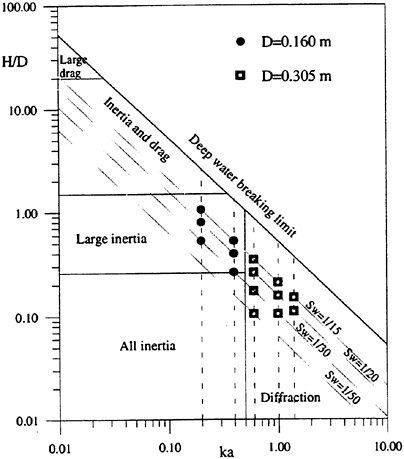
Figure 1. Present test cases ![]() .
.
Setup and experimental procedure
A cylindrical frame of reference has been adopted, as shown in Fig. 2. Wave elevation around the cylinder and pressure at the wall have been measured at 4 different radii and 4 different depths respectively for each selected azimuthal direction θ. Since most of the important features of the wave pattern were expected to be distinguishible in the near field, namely within a few radii from the cylinder wall, the maximum nondimensional distance r/a of the wave gauges from the cylinder axis has been set to 3 (D=0.305 m) and 4 (D=0.160 m) approximately while the first wave probe (WG1) has been placed as close as possible to the cylinder surface to obtain informations on the run-up profile. Table 2 summarises the positions of the measurement points. The measurements have been carried out for 0≤θ≤180 deg only.
The maximum error on the radial r and vertical coordinate z in Table 2 is 0.001 m.
For each pair (ka,Sw), the test was repeated varying the azimuthal direction θ of the sensors with angular step Δθ=10 deg. The maximum error in the azimuth is 0.5 deg. Summarizing, each test case of Table 1 is characterised by 76 wave elevation records and 76 pressure records. The interference between wave gauges and pressure transducers has been avoided shifting the wave gauges by 20 deg with respect to the pressure measurement angle.
Phase of the pressure and of the wave elevation is referred to the undisturbed incident wave measured at a fixed distance d=4.460±0.010 m from the cylinder axis on the wavemaker side.
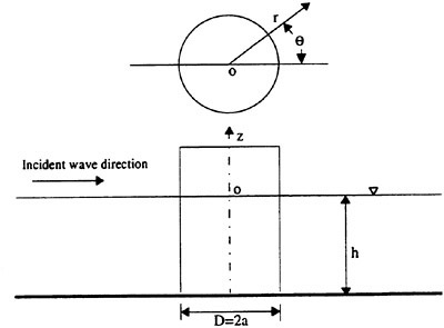
Figure 2. Schematic plot and frame of reference for the experiments.
Table 2.
|
D (m) |
Pressure |
z (m) |
Wave gauge |
r (m) |
r/a |
|
0.160 |
P1 |
−0.020 |
WG1 |
0.1050 |
1.3125 |
|
P2 |
−0.070 |
WG2 |
0.1750 |
2.1875 |
|
|
P3 |
−0.120 |
WG3 |
0.2450 |
3.0625 |
|
|
P4 |
−0.170 |
WG4 |
0.3150 |
3.9375 |
|
|
0.305 |
P1 |
−0.020 |
WG1 |
0.1830 |
1.2 |
|
P2 |
−0.070 |
WG2 |
0.2745 |
1.8 |
|
|
P3 |
−0.120 |
WG3 |
0.3660 |
2.4 |
|
|
P4 |
−0.170 |
WG4 |
0.4575 |
3.0 |
Quality of the incident waves
It is well known that the quality of the results of an experiment concerning the fluid-structure interaction depends on the quality of the ambient flow. Since most experimental tests, like those we are talking about in this paper, are aimed to determine the correlation between the main parameters of the exciting cause and the response of the system, no
meaningfull conclusions can be drawn from the tests unless the forcing cause is fully known. Moreover if the experiment is also aimed to validate theoretical numerical results, the experimental ambient flow must be given in detail and must be consistent with the theoretical one. In wavy flow, this corresponds to define the wave kinematics. In the case of regular waves, the ambient flow can be derived from the main parameters of the wave (period, length, height, profile or asymmetry parameters,…) by the use of consolidated wave models (9). In the case of strongly distorted waves the representation of the wave kinematics by the main parameters is not well extablished and some specific methods are usually adopted (Wheeler’s stretching,…).
The performances of the wave basin of the University of Trieste have been accurately analysed (10). A complete description of the quality of the waves in terms of the main parameters (height, period, harmonic composition,…) and associated uncertainty levels has been derived by means of specific tests. Summarising, it can be said that at the measurement station (L/2), the regular wave trains can be satisfactorily described by a third order Stokes wave provided the steepness Sw is less than 1/15 and an appropriate time window is applied to avoid reflection effects from the beach (11–13). The maximum deviations (a few units %) have been detected at the lowest frequencies and for the steepest waves.
Data acquisition and processing
Data were collected at a 100 Hz sampling rate. Time windowing of the signals has been applied in order to analyse only the steady state part of the records that are free from reflections from the side walls of the tank. The records were processed to give statistical informations, maxima, minima, bias, period and phase lag to the incident wave with their standard deviations. The frequency domain analysis has been performed on the same time window. Phase lag to the incident wave has been evaluated according to both the zero-up and the zero-down crossings to give evidence of possible asymmetry of the signals.
As stated before, uncertainty levels were estimated according to standard procedures given by ASME/ANSI (14) and to a certain extent we can say that this can be considered a novelty in the field. It was found that most of the global uncertainty comes from the not strict stationarity of the signal within the selected time window. This uncertainty is represented by the standard deviation of the maxima and minima shown in the plots of the results.
Finally, it must be stressed that the experimental results presented in the following are given in the form ![]() where σ is the standard deviation and
where σ is the standard deviation and ![]() is the mean value over Ν values. A 95% confidence interval URSS can be easily computed as
is the mean value over Ν values. A 95% confidence interval URSS can be easily computed as ![]() and the results represented in the more standard form
and the results represented in the more standard form ![]() . This simply comes from the application of the error theory when the bias error is always much lower than the repeatibility error and Ν is approximately 10.
. This simply comes from the application of the error theory when the bias error is always much lower than the repeatibility error and Ν is approximately 10.
Results
Most results of the experimental tests have been presented elsewhere and will not be shown here again because of lack of space.
Here the test cases G,H,I,J of Table 1 concerning ka=0.60 are shown in detail. The maxima and minima of wave elevation given in (m) and of the dynamic pressure given in (kPa) are presented in Figs. 6 to 9. The maximum and minimum wave elevation and the maximum and minimum dynamic pressure, are plotted vs. the azimuthal angle in the left and right column column respectively. From head to bottom, wave elevation data are ordered for increasing radius whereas pressure data are ordered for encreasing depth. Each data is reported with the confidence interval ±σ. In some test cases the pressure transducers at P1,P2 fully emersed in correspondence of the wave hollow: the dynamic pressure minima then becomes an unknown quantity in the range −ρgz(P1)÷−ρgz(P2) and −ρgz(P2)÷−ρgz(P3) respectively. In the figures, the dynamic pressure value has been set to the upper value of the given ranges, the error band corresponding to the noise of the signal.
Further results on the phase lag and on the other test cases can be found in Contento et al. (7).
NON-LINEAR NUMERICAL SIMULATION
Mathematical model
In the following, the wavy flow of an inviscid incompressible fluid generated by the interaction of a regular wave train with a vertical cylinder piercing the free surface Σ is studied. Upon assuming the flow irrotational, the velocity field ![]() can be expressed as the gradient of a potential Φ(Ρ, t) which satisfies the Laplace equation
can be expressed as the gradient of a potential Φ(Ρ, t) which satisfies the Laplace equation
(1)
in the flow domain, where P≡(x,y,z) is the vector position and t is the time. Beside this, the boundary conditions:
-
vanishing normal velocity on the wetted body Γ and on the bottom surface Ω;
-
constant pressure on the free surface Σ;
-
kinematic boundary condition on the free surface Σ are imposed and the initial values of Φ(Ρ,0) and are
 prescribed.
For the purpose of numerical solution, it is expedient to split the potential Φ(P, t) in the form
(2)
where φ is the velocity potential of the incoming unperturbed wave and ![]() is the perturbation induced by the presence of the body. In the following, the incident wave field is given by a two-dimensional Stokes wave which can be computed accurately as described in (16) Consistently, we use the initial conditions
is the perturbation induced by the presence of the body. In the following, the incident wave field is given by a two-dimensional Stokes wave which can be computed accurately as described in (16) Consistently, we use the initial conditions
(3)

(4)
that is the body suddenly appears at t=0. Although the following transient is not realistic, the decomposition (2) allows for obtaining steady regime results without simulating a numerical wavemaker. As discussed in (15,17), the above split is just a change of the unknown variable and, by properly manipulating the relevant equations, no approximations are introduced in the continous problem. Instantaneous pressures on the cylinder are given by the Bernoulli theorem
(5)
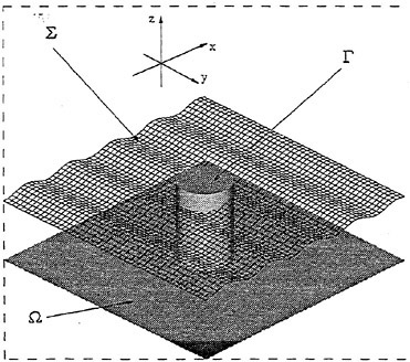
Figure 3. Schematic plot of the computational domain
Numerical model
The numerical scheme adopted is extensively discussed in (3,15) and here just a brief description is recalled. The perturbation potential ![]() is expressed through the simple layer potential
is expressed through the simple layer potential
(6)
where G(P, P*) is the free space Green function for the Laplace operator and σ is the source strength. In the integral (6), the physical boundary Δ consists of the wetted part of the body surface Γ, the free surface Σ and the bottom Ω. The latter is the only portion of the boundary domain that remains unchanged during the evolution, while the free surface and the wetted surface of the body change in time.
In the numerical solution the surface Γ of the cylinder is discretized into Ν quadrilateral panels, on which the source distribution is assumed piecewise constant. Unlikely, on Σ, the simple layer distribution is replaced by Μ point-sources ![]() displaced above the free surface with variable desingularization distance zi. chosen according to (18) as follows
displaced above the free surface with variable desingularization distance zi. chosen according to (18) as follows
(7)
where Ai is the surface portion assigned to the i-th source. The parameters α and ß are computed once and for all through a preliminary optimization procedure, which for small wave amplitudes allows to recover numerically the analytical solution (2). The effect of the bottom is accounted for through the method of images and, consistently, the discretized integral representation of the perturbation potential reads
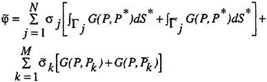
(8)
where Γj and σj are the j-th panel on the body surface and the corresponding source density, ![]() is the mirror image of Γj-with respect to the bottom.
is the mirror image of Γj-with respect to the bottom.
Ρk denotes the location of the k-th source ![]() above the free surface and
above the free surface and ![]() is the corresponding image.
is the corresponding image.
The physical points on the free surface as well as the sources ![]() are distributed on an unstructurated mesh in which the radial and circumferential spacings are approximately uniform.
are distributed on an unstructurated mesh in which the radial and circumferential spacings are approximately uniform.
Once the integral equations following from (8) are solved, the velocity field on Σ can be evaluated by taking its gradient and the free surface can be simply updated in time by using a fourth order Runge-Kutta scheme. Filtering techniques are applied to avoid small scale instabilities and damping terms in the kinematic and dynamic evolution equations are introduced to prevent unphysical reflections at the edge of the computational domain.
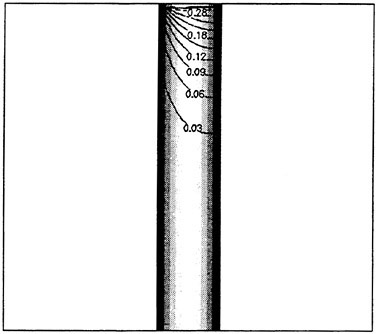
Figure 4. Pressure distribution during the simulation
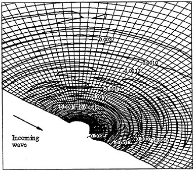
Figure 5. Wave pattern during the simulation.
COMPARISON BETWEEN EXPERIMENTAL, LINEAR ANALYTIC AND NON-LINEAR NUMERICAL RESULTS
a) Linear theory
In this paper the comparison between the experimental results and the exact linear theory is limited to the test cases G-H-I-J, i.e. ka=0.60. Full details about other ka values can be found in Contento et al. (7). Summarising, in each test case the comparison between measured and predicted amplitudes and phase lags is particulary meaningfull. First of all the linear diffraction theory confirms its good work for ka≥0.6 and small to moderate wave steepness Sw≤1/30. The goodness of the predictions is both qualitative (azimuthal position of the bumps and hollows in the maxima and minima) and quantitative (amplitudes and phase). An increasing steepness makes the comparison less good mostly at the point P1, i.e. in proximity of the calm water level. Moreover a general disagreement appears in the phase lag.
In the test case J (ka=0.60, Sw=1/50), the comparison between the experimental results and those from the linear theory is extremely good whereas with the maximum steepness (test case G), some discrepancies appear in the pressure minima at P1 due to the full emersion of the sensor. The pressure maxima are generally overpredicted by the linear theory. Higher order effects are expected to be responsible for the asymmetry between maxima and minima.
As far as the wave elevation is concerned, some bumps in the curve representing the maximum wave elevation are missing in the linear results in the range 0°≤θ<90° and some more problems are encountered in the wave minima that are generally overestimated by the linear theory.
To highlight the observed deviations from the linearity, the 76 time records of each test case have been processed by a Fourier analysis. In Figs. 6 to 9 the first three harmonic components are plotted. As expected, the results of the linear theory are closer to the first harmonic component than to the global experimental results. The higher order components are however quite large and remain unexplained in the frame of the linear approach.
b) Non-linear numerical results
The results of the non-linear computations are plotted in Figs. 6 to 9 and compared with the experimental data and with the linear analytic predictions. Numerical computations have been performed by using 58 panels deepwise and 15 panels circumferencewise on the body (uniformly spaced) and about 6000 source points on the free surface. The
maximum and the minimum are computed by considering the periodic relief.
Computed wave elevation profiles show a very good agreement with the experimental wave pattern. For increasing wave steepness, the agreement gets slightly worst, particularly for the first two stations WG1 and WG2 (closest to the body). The amplitude of the second and third Fourier modes of the experimental data indicates the presence of non negligible non-linear effect. It is important to observe that the numerical data on the wave elevation are in a good agreement with the experiments even when nonlinear effects are relevant, allowing to state that the numerical scheme is well suited to capture non-linear wave effects.
As far as the numerical prediction of the wall pressure on the cylinder is concerned, some remarks must be done on the available experimental data. It has been already observed that in the case of steep waves (test cases G-H), the pressure probes P1 and P2 fully emersed during part of the wave period. In this case the experimental value of the minimum dynamic pressure has been set to the hydrostatic one (−ρgz(P1)). On the contrary, when the full emersion of the control point P1 occurred (test cases G-H), no value of the dynamic pressure has been assigned to the numerical results therefore these values are not shown in the figures. For all other cases, the agreement with the experiments is quite good, strictly following bumps and other nonlinear features. In particular the simulation of the maximum run-up is touching even in the worst cases.
Finally it must be highlighted that dispite the coarseness of the grid used on the cylinder wall, the pressure results are rather good anyhow.
CONCLUSIONS
Some results of a research project developed in the frame of the cooperation between DINMA and INSEAN have been presented.
Most objectives of the project have been successfully reached, namely an highly accurate experimental investigation on the local interaction between a wavy flow and a vertical pile in diffraction regime, the confirmation of the applicability limits of the exact linear theory and the performance of a well based validation procedure for a fully non-linear numerical code developed in this context.
In any case, the presented non-linear numerical results are very preliminary ones but very encouraging too. The validation of the code against the other data, here not shown, is still in progress and looks promising as well. Some refinements are still needed in the crest/through zone. The validation, carried out under the light of very detailed sets of experimental data, is allowing many indications of the reasons of some minor discrepancies and of the action to be taken to eliminate them.
Summarizing the preliminary results about the other ka conditions not reported in this paper, it can be said that higher order effects appear in the crest-hollow zone for the small ka numbers, namely ka=0.20, 0.40. Faltinsen et al. (19) have shown that second and third order pressures with comparable amplitude have to be accounted for in flow conditions like these. Higher order effects also appear in the full diffraction regime with ka=1.00 and 1.40 and with the largest wave steepness tested (Sw=1/15). In agreement with Kriebel (5), we have also found that in steep waves, as far as the run-up is concerned, linear theory underpredicts the experimental results by 44% on average (up to 80 % in some cases).
AKNOWLEDGEMENTS
The experimental work has been supported by INSEAN in the frame of the cooperation between DINMA and INSEAN, Contract Code 2/LR 343/95 of the Research Plan 1994–96.
The numerical work has been supported by the Italian “Ministero dei Trasporti e della Navigazione” in the frame of INSEAN research plan 1994–96. Daniele Peri wishes to thank M.Greco, M. Landrini and C.Lugni (INSEAN) for some numerical tools provided to develop the reported computations.
LIST OF SYMBOLS
|
a |
cylinder radius (D=2a) |
|
d |
distance between the cylinder axis and the incident wave gauge |
|
g |
gravity acceleration |
|
h |
depth of water in the wave basin |
|
k |
wave number |
|
p |
dynamic pressure |
|
r,θ,z |
cylindrical coordinates in the experiments |
|
t |
time |
|
|
velocity field |
|
Ai |
area associated with the source |
|
B |
breadth of the wave basin |
|
G(P,P*) |
Green function |
|
H |
undisturbed incident wave height |
|
L |
lenght of the wave basin |
|
N |
number of maxima/minima within the time window |
|
P |
vector point in the computations |
|
Pi |
label of the measurement point i for p |
|
Sw |
wave steepness (Η/λ) |
|
URSS |
95% confidence interval |
|
T |
wave period |
|
WGi |
label of the measurement point i for η |
|
α |
desingularization parameter |
|
β |
desingularization parameter |
|
φ |
incident wave potential |
|
|
perturbation potential |
|
Φ |
total potential |
|
η |
total wave elevation in the experiments and incident wave elevation in the computations |
|
|
wave elevation corresponding to the perturbation potential |
|
λ |
wave length |
|
Γ |
body surface |
|
Δθ |
angular step of the azimuth θ angle σ standard deviation |
|
σ(P) |
source strenght |
|
Δ |
computaional fluid domain |
|
Σ |
free surface |
|
Ω |
bottom surface |
REFERENCES
1. Morison, J.R., O’Brien, M.P., Johnson, J.W, Schaff, S.A., “The Force Exerted by Surface Waves on Piles”, Petroleum Trans., AIME, Vol. 189, 1950, pg. 149–157.
2. Mac Camy, R.C., Fuchs, R.A., “Wave Forces on Piles: A diffraction Theory”, U.S. Army Corps of Engineering, Beach Erosion Board, Tech. Memo, No. 69, 1954, Washington D.C.
3. Lalli, F., Di Mascio, A., Landrini, M., “Nonlinear Diffraction Effects Around a Surface-Piercing Structure”, Int. Journal of Offshore and Polar Engineering, Vol. 6, No. 2, 1996.
4. Hogben, N., Standing, R.G., “Experience in Computing Wave Loads on Large Bodies”, Proceedings of the Offshore Technology Conference, Dallas, Texas, 1975.
5. Kriebel, D.,L., “Nonlinear Wave Interaction with a Vertical Circular Cylinder. Part II: Wave Runup”, Ocean Engineering, Vol. 19, 1992, pp. 75–99.
6. Francescutto, A., Tan, P., “Considerations on the Applicability of ISO9000 to Seakeeping”, Report nº 27, 1995, Dept. of Naval Architecture, Ocean and Environmental Engng, University of Trieste, Italy.
7. Contento, G., Francescutto, A., Lalli, F., “Non-linear Wave Loads on Single Vertical Cylinders: Pressure and Wave Field Measurements and Theoretical Predictions”, 1998, to appear on the Proceedings of the 8th Int. Conference on Offshore and Polar Engineering ISOPE’98, Montreal, Canada.
8. Chakrabarti, S.K., “Nonlinear Methods in Offshore Engineering”, 1990, Elsevier, New York.
9. Wiegel, R.L., “Oceanographical Engineering”, 1964, Prentice Hall Inc., Englewood Cliffs, New Jersey 07632.
10. Codiglia, R., Contento, G., Francescutto, A., “Measurement of the Fundamental Parameters of Regular Waves in the Wave Tank of DINMA: Uncertainty Analysis and Error Propagation on the Wavemaker Calibration”, Report nº 35, 1998, Dept. of Naval Architecture, Ocean and Environmental Engng, University of Trieste, Italy.
11. Fryer, D.K., Gilbert, G.G., “The Useful Lenght of a Ship Tank”, Int. Shipbuilding Progress, Vol. 36, nº 408, 1989, pp. 385–403.
12. Fryer, D.K., Mitchell, J.E., “A Wave Absorber for Ship Tanks and Seakeeping Model Test Basins”, Int. Shipbuilding Progress, Vol. 38, 1991, pp. 393–410.
13. Nallayarasu, S., Hin Fatt, C., Shankar, N.J., “Estimation of Incident and Reflected Waves in Regular Wave Experiments”, Ocean Engineering, Vol. 22, 1995, pp. 77–86.
14. Coleman, H.G., Steele, W.G., “Engineering Applications of Uncertainty Analysis”, tutorial outline given at ASME Fluid Engineering Division Annual Meeting, 1997, Vancouver.
15. Di Mascio, A., Landrini, M., Lalli, F., Bulgarelli, U., “Three dimensional Nonlinear Diffractrion Around a Fixed Structure”, Proceedings of the 20th Symposium of Naval Hydrodynamics, 1994, Santa Barbara (California).
16. Schwartz, L.W., “Computer Extension and Analytic Continuation of Stokes Expansion for Gravity Waves”, Journal of Fluid Mechanics, Vol. 62, 1974. p. 553–578.
17. Landrini, M., “Fenomeni non lineari nella propagazione di onde di superficie libera” (in Italian), Ph. D. Thesis, 1994, Universisty of Rome “La Sapienza” .
18. Cao, Y., Schultz, W.W., Bech, R.F., “Three-dimensional Desingularized Boundary Integral Methods for Potential Problems”, Int. Journal on Numerical Methods in Fluids, Vol. 12, 1991, p. 785–803.
19. Faltinsen, O.M., Newman, J.N., Vinje, T., “Nonlinear Wave Loads on a Slender Vertical Cylinder”, Journal of Fluid Mechanics, Vol. 289, 1995, pp. 179–198.
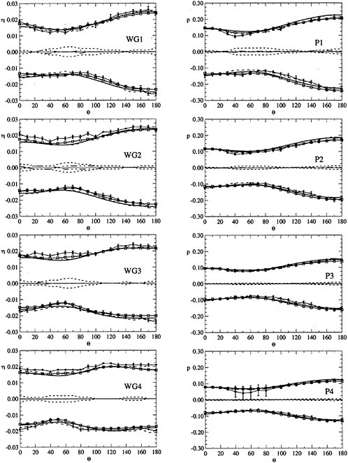
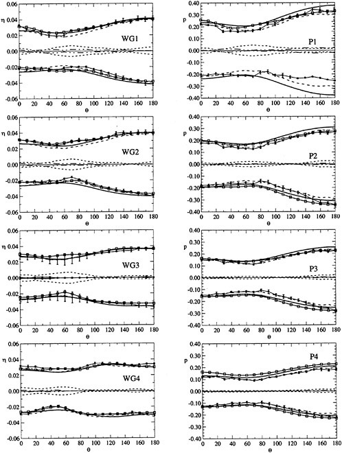
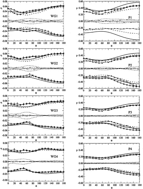
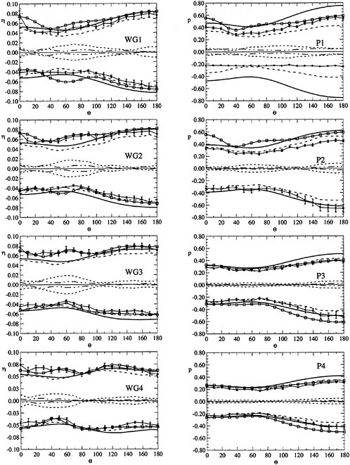
DISCUSSION
C.Stansberg
Norwegian Marine Technology Research Institute, Norway
The paper presents a set of well conducted experiments on wave diffraction and corresponding hydrodynamic pressures around a vertical column, compared to linear and nonlinear theoretical/numerical predictions. Inviscid fluid is assumed. The results show that for moderately steep waves, linear diffraction theory works well, and the fully nonlinear model reconstructs these cases satisfactorily. In the steeper wave conditions, however, the measurements show systematic deviations from linear theory. This is as expected. To some extent, the nonlinear model here follows the same trend as the measurements, but there are also discrepancies. Thus the predicted pressure minima, e.g., are systematically more negative than the measured ones. Could this, and other observed discrepancies, be commented on? Have the authors made any comparisons to, e.g., fully second-order diffraction models?
It is particularly interesting to notice the significantly nonlinear behaviour in the pressure sensor P1 in test cases G and H, where the measured (total as well as 1st harmonic) as well as predicted nonlinear maxima are clearly lower than the linear prediction. At the same time, the measured 3rd harmonic is getting quite high, about as high as the 2nd harmonic. Could these nonlinear effects be seen in connection with, e.g., “ringing” phenomena? (And how do the authors estimate Fourier harmonics from pressure signals that have truncated minima?) It could also be interesting to see graphs with predicted vertical pressure maxima profiles (p vs. z), compared to measurements. Pressure measurements at z>0 would also have been very interesting if they had been available, and they are suggested for possible future studies. Similarly, parallel measurements (and calculations) on integrated forces and moments could also be included in the future, for easier comparisons to some of the published works. A set of such measurements on different vertical columns has been recently presented and analyzed in Stansberg [1],
[1] Stansberg, C.T. (1997), “Comparing Ringing Loads from Experiments with Cylinders of Different Diameters—An Empirical Study,” Proceedings, Vol. 2, the BOSS’97 Conference, Delft, The Netherlands, July 1997.
AUTHORS’ REPLY
We thank Dr. Stansberg very much for his very interesting discussion and for the suggestions for future work. The causes of the discrepancies between the numerical and experimental results in the comparison of the pressure on the cylinder, observed by Dr. Stansberg, are presently under investigation. As a part of this analysis, the comparison between the presented nonlinear code and a second order one will be carried out. At the moment, some work based on a fully second-order model is in progress at INSEAN [1].
Now referring to the nonlinear behaviour of the measured as well as computed maxima of the dynamic pressure at the position P1 in the test cases G and H and in particular to the magnitude of the 3rd harmonic component of the experimental data, it has been observed by Dr. Stansberg that the time history of the pressure signal exhibits truncated minima due to the periodic emergence of the transducer. Obviously this would have been the same for any other pressure sensor position in the crest-hollow zone. In these cases the discontinuity in the first derivative of the pressure signal unavoidably corresponds to higher order Fourier components. Faltinsen et al. [2] have shown that for a slender cylinder with a radius/wave amplitude ratio of order O(1), second and third order terms in the total force appear in the free surface zone due to the first order and nonlinear potential. There, the contributions connected with different wave-body interaction effects have been derived separately. In our case it is not easy to transform the local load measured at the pressure sensor in the integral quantities responsible for the “ringing” phenomenon. As a consequence, the connection between the higher order components of the local loads derived by Fourier analysis and the “ringing” of the structure is not completely clear. Further investigations are planned.
[1] Lugni, C., Landrini, M., Graziani, G., “Un modello debolmente nonlineare per l’idrodinamica di una struttura galleggiante,” (in Italian) XIII Cong. Naz. AIMETA, Siena, 1997.
[2] Faltinsen, O.M., Newman, J.N., Vinjie, T., “Nonlinear Wave Loads on a Slender Vertical Cylinder,” Journal of Fluid Mechanics, vol. 289, pp. 179–198, 1995.
Validation of a Chimera RANS Method for Transient Flows Induced by a Full-Scale Berthing Ship
H.-C.Chen (Texas A&M University, USA)
E.Huang (Naval Facilities Engineering Service Center, USA)
ABSTRACT
A chimera Reynolds-Averaged Navier-Stokes (RANS) method has been developed for time-domain simulation of transient flow induced by a ship approaching a berthing structure. The method solves the mean flow and turbulence quantities on embedded, overlapped, or matched multiblock grids. The unsteady RANS equations were formulated in an earth-fixed reference frame and transformed into general curvilinear, moving coordinate systems. A chimera domain decomposition technique has been employed to accommodate the relative motions between different grid blocks. Calculations have been performed for a 1/8-scale model barge and a full-scale motor vessel in berthing operations. Comparisons have been made between the computations and measurements to demonstrate the feasibility of the chimera RANS approach for time-domain simulation of the hydrodynamic coupling between the ship and berthing structures. The numerical solutions successfully captured many important features of the transient flow around a berthing ship including the underkeel flow acceleration, wake flow separation, and water cushion between the ship and harbor quay wall.
INTRODUCTION
Berthing damage can result in substantial economic and operational penalties. Even in a well executed berthing, a large ship possesses enormous kinetic energy that could seriously damage the berthing structure as well as the ship itself. Fender systems are provided at a berth to absorb the kinetic energy of the berthing ship and to mitigate impact forces. In order to improve the design of berthing facilities, it is desirable to develop a reliable hydrodynamic assessment system for accurate time-domain simulation of the berthing processes which involve complex interactions among the ship, the fender system, and arbitrary harbor floor bathymetry. Recently, Chen, Chen and Davis [1], Chen, Chen and Huang [2] Chen, Chen, Davis and Huang [3], and Chen and Chen [4] developed a chimera RANS method for the simulation of transient flows induced by berthing operations of practical ships in fully sheltered harbors. The method solves the mean flow and turbulence quantities on embedded or overlapped grids using a domain decomposition approach. Calculations have been performed for a DDG-51 ship in combined translational and rotational motions to demonstrate the capability of the chimera RANS method for time-domain simulation of berthing ships. The numerical solutions successfully captured many important features of transient flow around a berthing ship including the underkeel flow acceleration, wake flow separation, water cushion between the ship and harbor quay wall, and the complex interactions between the bow, shoulder, and stern waves. A direct validation of the accuracy of these simulation results, however, was not possible due to the lack of experimental data.
In order to verify the accuracy of the chimera RANS method for berthing simulations, model experiments have been conducted recently by Huang, Davis, Kim and Chen [5], [6] in a shallow water basin using a 4.572 m (15 ft) barge model. Current meters and wave gages were used to measure the fluid velocities and wave elevations at selected locations along the path of the berthing barge. Time-domain simulations have been performed for the berthing barge at various approaching speeds and water depths to evaluate the accuracy and overall capability of the chimera RANS method.
To further assess the general performance of the chimera RANS method for practical berthing operations, a series of full-scale experiments have been conducted by Davis, Huang and Hatch [7] recently at a small harbor in Port Hueneme, California using a 57.30 m (188 ft) long ship. Current meters were placed at ten selected locations along the path of the berthing ship to measure the longitudinal, transverse, and vertical components of the fluid velocities. Time-domain simulations have been performed for the berthing ship under prescribed motions to identify the important parameters and flow features associated with berthing operations. Comparisons have been made between the calculated and measured time histories of velocity variations to illustrate the general capability of the present method.
CHIMERA RANS METHOD
In the present study, the chimera RANS method of Chen, Chen and Davis [1] and Chen and Chen [4] has been employed for time-domain simulation of transient flow induced by a berthing ship. In this approach, the transport equations for both momentum and turbulence quantities are solved using the finite-analytic method of Chen, Patel, and Ju [8]. To solve for the pressure, the SIMPLER/PISO pressure-velocity coupling technique of Chen and Patel [9] and Chen and Korpus [10] is used. A brief summary of the governing equations and solution procedures is provided in this section.
Governing Equations
Consider the nondimensional Reynolds-Averaged Navier-Stokes equations for incompressible flow in orthogonal curvilinear coordinates (xi, t)=(x1, x2, x3, t)
(1)
(2)
where Ui and ui represent the mean and fluctuating velocity components, and gij is conjugate metric tensor, t is time, p is pressure, and Re=UoL/ν is the Reynolds number based on a characteristic length L, a reference velocity Uo, and the kinematic viscosity ν. Equation (1) represents the continuity equation and equation (2) represents the mean momentum equation. The equations are written in tensor notation with the usual summation convention assumed. The subscripts, ,j and ,jk, represent the covariant derivatives.
In the present study, the two-layer turbulence model of Chen and Patel [11] is employed to provide closure for the Reynolds stress tensor ![]() . In this approach, the Reynolds stresses are related to the corresponding mean rate of strain through an isotropic eddy viscosity νt,
. In this approach, the Reynolds stresses are related to the corresponding mean rate of strain through an isotropic eddy viscosity νt,
(3)
with
(4)
(5)
where eij represent the contravariant components of the rate-of-strain tensor, and k is the turbulent kinetic energy. Substituting equation (3) into (2) yields:
(6)
The quantity 1/Ru=1/Re+νt/σu represents the effective eddy viscosity. The eddy viscosity can be computed from the turbulent kinetic energy k and its dissipation rate ε:
(7)
The turbulence quantities k and ε are solved using the following transport equations:
(8)
(9)
where the production term, G, is:
(10)
and the coefficients (Cμ, Ce1, Ce2, σu, σk, σe)=(0.09, 1.44, 1.92, 1.0, 1.0, 1.3). The effective viscosities in equations (8) and (9) are taken as 1/Rk=1/Re+νt/σk, and 1/Re=1/Re+νt/σe, respectively.
In the near wall region, turbulent fluctuations are affected by the wall. To account for the wall effects, the two-layer approach of Chen and Patel [11] is used. In the region away from the wall, the two-equation k-ε model described previously is applied. Close to the wall, the dissipation rate is determined from the turbulent kinetic energy and the dissipation length scale ℓe as follows:
(11)
(12)
Using this relationship, the turbulent kinetic energy can be determined from equation (8) with the following eddy viscosity distribution:
(13)
(14)
Numerical Method
To use the equations presented previously, they must be transformed into body-fitted coordinates from the orthogonal curvilinear coordinate system (x1, x2, x3, t). The body-fitted coordinate system is generally a non-orthogonal curvilinear coordinate system (ξ1, ξ2, ξ3, τ). The above transport equations for U(i), k, and ε are discretized using the finite-analytic approach of Chen, Patel and Ju [8]. Note that U(i)=hiUi are the physical components of the contravariant velocity vectors defined in terms of scale factors hi. Each transport equation is rewritten in the form of a general convection/diffusion equations:
(15)
In the finite-analytic approach, equations (15) are linearized in each local element of dimensions Δξ1=Δξ2=Δξ3=2 and solved analytically by the method of separation of variables. Evaluation of the analytic solution at the interior node provides a stencil for the center point in terms of its nearest neighbors. Using Euler implicit differencing in time, and lumping streamwise influences into single points upstream and downstream of P, results in a twelve-point discretization formula:
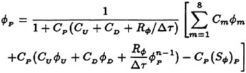
(16)
Subscripts ‘U’ and ‘D’ represent points in the stencil upstream and downstream of P, and subscripts ‘m’ (m=1, 8) represent the eight nearest points to Ρ in the cross-flow plane. Expressions for the finite-analytic coefficients (CP, CU, CD, Cm) can be found in Chen, Patel and Ju [8].
Pressure/velocity coupling is accomplished using the hybrid SIMPLER/PISO algorithm of Chen and Patel [9] and Chen and Korpus [10]. The approach introduces contravariant pseudovelocities at staggered locations, but leaves pressure (and all other dependent variables) at the grid nodes. The resulting computational cell for pressure has dimensions of Δξ1=Δξ2=Δξ3=1 centered on the regular grid nodes. By requiring the contravariant velocity field, Vi, to satisfy the equation of continuity:

(17)
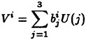
(18)
a pressure equation can be derived in terms of pseudovelocities ![]() as follows:
as follows:
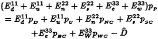
(19)
where
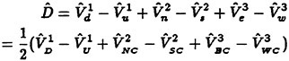
(20)
As before, subscripts refer to points in the stencil around P, with lower case letters indicating the staggered locations of the pseudovelocities on different faces of the control volume. A more detailed description of the SIMPLER/PISO pressure solver are given in Chen and Patel [9] and Chen and Korpus [10].
General Solution Procedure
In the present chimera RANS method, the solution domain is first decomposed into a number of computational blocks. The body-fitted numerical grids for the ship and the harbor fluid domain are generated separately with the ship grid blocks completely embedded in the harbor grid. The ship grids are allowed to move with a prescribed velocity relative to the harbor grid in arbitrary combinations of translational and rotational motions. The PEGSUS program (Suhs and Tramel [12]) is employed every time step to determine the interpolation information for linking grids. It outputs a complete set of information corresponding to the interpolation performed. The most important information is included in the IBLANK array, the interpolation and boundary lists, the interpolation stencils, and the maps showing boundary and interpolation node locations. The IBLANK array and interpolation stencils are incorporated into the present chimera RANS code to remove the hole points and update boundary conditions from the linking grids.
The overall solution procedure consists of an outer loop over time and an inner loop or sweep that iterates over the blocks of the grid. The discretization equations for pressure, velocity, and turbulence quantities form a system of tridiagonal matrices which was solved using an iterative ADI scheme. When a point is classified as a hole point (IBLANK=0) it must be removed from the solution process. To do this, the value at the hole point must remain unchanged over a time step to avoid affecting the solution. This is achieved by setting the diagonal elements to 1 and off-diagonal elements to zero in the tridiagonal matrix at the hole points. The points classified as hole boundaries also have an IBLANK value of 0, which removes them from the solution process. These values, however, must be updated by interpolated values from another grid. To ensure the proper conservation of mass and momentum between linking grid blocks, the grid-interface conservation technique of Hubbard and Chen [13] has been employed to eliminate unphysical mass source resulting from the interpolation errors. More detailed description of the chimera RANS/free surface method and the associated data management system are given in Hubbard and Chen [13], [14].
For unsteady problems involving relative motions between different grid blocks, the solution procedure can be summarized as follows:
-
Construct the initial grids for each component of the configuration.
-
Construct a boundary condition table specifying appropriate boundary conditions for each face.
-
Specify the initial conditions for velocity, pressure, and turbulence fields.
-
Determine interpolation information for linking grids using the PEGSUS program.
-
Calculate the geometric coefficients.
-
Calculate finite analytic coefficients and source functions.
-
Solve the momentum equations (U(i)) and turbulence equations (k, ε) using the iterative ADI scheme.
-
Calculate the pseudovelocities
 and calculate pressure (p) using the iterative ADI scheme.
 -
Repeat steps 7 and 8.
-
Move grids to new position to accommodate the prescribed ship motions.
-
Return to step 4 for next time step.
RESULTS AND DISCUSSION
As noted earlier, the chimera RANS/free-surface method has been employed recently by Chen, Chen and Davis [1], and Chen and Chen [4] for time-domain simulation of transient flow induced by two- and three-dimensional berthing ships in prescribed translational and rotational motions. In the present study, extensive calculations have been performed for a model-scale barge and a full-scale ship and compared with the available measurements to evaluate the general performance of the present method.
Validations for a Model-Scale Barge
The present chimera RANS method was validated first for a 4.572 m (15 ft) barge model tested by Huang, Davis, Kim and Chen [5], [6]. Figure 1 shows the experimental setup for the 1/8-scale barge model in a shallow water wave
basin located at Texas A & M University. The length, width, and draft of the barge at the waterline are (L, W, D)=(4.365 m, 0.955 m, 0.17 m). Calculations have been performed for three different water depths of h=0.35 m, 0.26 m, and 0.21 m corresponding to the experimental conditions. For brevity, we shall present only the results for the deepest water case here. Figure 2 shows the computational domain and numerical grids for the h=0.35 m case at the beginning and end of the simulations. The 31×21×41 barge grid is allowed to move with respect to the 31×251×21 basin grid according to the measured barge speed. As noted in Huang et al. [5], the towing carriage could not move the barge forward at a constant speed due to surface irregularities of the guiding rails. As a result, the actual approach speed of the barge varied typically within 15 percent of the target speed as shown in Figure 3. This has produced a somewhat more complicated flow field than desired. In addition, strong electrical noises were also picked up while recording raw data. This high frequency noise was successfully screened from current measurement by a low-pass filter. It was further noted in Huang et al. [5] that the barge was too heavy for positive handling by the towing carriage. As the barge decelerated to a quick stop before the quay wall, its stopping produced pronounced vertical vibration, including a dominating current activity that is not a normal characteristic of actual berthing operations. Nevertheless, the general flow pattern was sufficiently clear to guide the development of the numerical simulation techniques.
In the present simulation, the barge motion was approximated by constant forward speed and ramp start/stop (see Figure 3) to eliminate the unwanted fluctuations caused by the jerky movements of the towing carriage. For simplicity, the barge was assumed to accelerate gradually from 0 to 10 cm/s during 0≤t≤4.55 s, maintaining a constant speed of Uo=10 cm/s between t=4.55 s and 63.02 s, and then decelerated to zero speed from t=63.02 s to 65.29 s. A total of 320 time steps was used with a constant time increment of 0.2275 sec (or dimensionless time increment ΔtUo/L=0.005). At the end of the simulation, the barge has traveled a total distance of 5.94 m, or 1.36 barge length. Since the general flow features are similar to those shown in Chen et al. [15] for the shallowest water case of h=21 cm, we shall present here only the time history at selected measurement stations shown in Figure 3 to illustrate the predictive capability of the present method.
It is seen from Figure 3 that the present results are in very good agreement with the measurement except for some discrepancies after the barge touched the fender. As noted earlier, the barge experienced heave and roll motions during the deceleration stage because the towing carriage was not strong enough to absorb the kinetic energy caused by the impact. The observed oscillations in the measured velocities are most likely due to the presence of heave and roll motions which were not modeled in the present numerical simulations. In spite of these uncertainties, the present results clearly demonstrated the predictive capability of the chimera RANS method for time-domain simulation of transient flow induced by barge motions.
Validations for a Full-Scale Ship
After successful validations for the berthing barge, the present method was further extended for the calculations of transient flow induced by a full-scale motor vessel (Μ/V) named Independence. A series of experiments were conducted by Davis, Huang and Hatch [7] in a small harbor at Port Hueneme, California to collect essential data for transient flow field encountered during berthing operations. Figure 4 illustrates the general layout of the experimental facility. The ship length at the designed waterline (DWL) is 57.3 m (188 ft), and the ship draft varies slightly between 3.56 m and 3.58 m. Current meters are placed at ten different locations along the ship path as also shown in Figure 4. In the present chimera domain decomposition approach, a 61×31×51 body-fitted numerical grid was constructed for accurate resolution of the turbulent boundary layer flow around the ship hull. This grid topology requires the use of a branch cut along the front center plane where appropriate boundary conditions must be provided. In the present multiblock approach, a small 5×31×26 grid was constructed to enclose the branch cut so that the flow field along the front center plane can still be computed directly from the RANS equations. The second block is fully embedded in the first ship grid with exact point-to-point matching to ensure complete continuity of the solutions between the two ship grids.
In the present berthing simulations, the harbor is covered by two computational grid blocks
as shown in Figure 5. The larger block consists of 61×121×21 nodal points while the smaller block has 25×42×21 points. The water depth varies between 7 ft and 38 ft under mean low water (MLW) level condition. The geometric complexity of the ship hull and harbor bathymetry makes the construction of fully-connected grids very difficult and time-consuming even in the absence of ship motions. On the other hand, the chimera domain decomposition method enables us to accommodate arbitrary translational and rotational motions without tedious adaptive generation of body-fitted numerical grids at each time step. Figure 5 shows also the intial and final ship positions and the corresponding chimera numerical grids. It is noted that part of the numerical grids (i.e., hole points) for the harbor blocks have been removed from the computational domain using the PEGSUS program of Suhs and Tramel [12].
Calculations were performed for the motor vessel Independence in lateral motions under four different flow conditions: X650D, X750A, X750B, and X825A. Figure 6 shows the time history of ship speed for all four test cases considered. For the sake of brevity, however, we shall present detailed numerical results for only the X650D case. For this test case, the ship draft is 3.58 m (11.75 ft) and the tide is 1.16 m (3.8 ft) at the time of the test. Calculations were performed for 300 time steps using a constant time increment of 0.988 sec (dimensionless time ΔtUo/L=0.002). This corresponds to t=157–453.4 sec in the measured time history as the ship remained stationary until t=157 sec. For simplicity, the free surface effects were neglected although the present method is capable of handling free surface waves as demonstrated in Chen and Chen (1998). This is well justified since the Froude number based on the maximum ship approach speed and vessel length is less than 0.005.
Figures 7 and 8 show the contours of the computed lateral (parallel to harbor quay wall) and inline (in the direction of ship motion) velocity contours at several different time instants of t=255.8 s, 305.2 s, 354.6 s, and 453.4 s to illustrate the general characteristics of the transient flow field induced by the ship berthing operation. Note that the velocity on the hull surface is identical to the ship approach speed in the present earth-fixed reference frame. It is further noted that the flow behind the ship moves faster than the ship which indicates the presence of a recirculation region. The recirculation flow pattern can also be clearly seen from the top view of the free surface velocity vectors shown in Figure 9.
In order to provide a more detailed description of the unsteady three-dimensional flow induced by the berthing operations, we shall also present the velocity vector plots at two different cross sections as shown in Figures 10 and 11. At the station Χ/L=0.42 near the midship, it is clearly seen that the sharp corners of bilge keels have led to a rather complex flow separation and reattachment pattern in the direction of the ship motion. During the acceleration and constant speed stages from t=157 s to t=344 s, the downstream bilge keel produced a large recirculation region behind the ship as seen in Figure 10(a)–(d). After the ship touched the fenders, the trailing water flow continued to move towards the harbor quay wall and force the water into the underkeel clearance between the bottom of the ship and harbor floor. It is seen from Figure 10(e)–(g) that the movement of trailing water has resulted in a strong vortical flows adjacent to the ship side wall. Moreover, the momentum of the trailing water also forced some of the water to move into the underkeel region and the gap between the fenders and the harbor quay wall. Since the current changes direction in the underkeel region, the flow separation and reattachment regions were seen to occur in different sides of the bilge keels when comparing to those observed earlier before fender impacts.
It is interesting to note that the flow patterns at Χ/L=0.92 in the stern region (Figure 11) are considerably different from those observed near the midship. During the ship acceleration and constant speed stages, the skeg produced a single recirculation region behind the ship path. After the fender impacts, the trailing water was forced to move under the skeg and produced a counterclockwise vortex in the opposite direction. Since the local water depth is quite deep at this station, the effects of harbor floor is rather small in comparison with those observed near the midship.
For completeness, the pressure contours at selected time instants are also shown in Figure 12 to provide a more detailed description of the unsteady three-dimensional flows around the berthing ship. During the acceleration and constant forward motions, a high pressure region was observed ahead of the ship around the front stag-
nation point. Moreover, strong negative pressures were predicted in the recirculation region behind the ship due to longitudinal flow separations. When ship touched the fenders, however, the high pressure region was seen to shift to the other side of the ship as the trailing water continues to push the ship towards the fender system. This shift of hull pressure distributions has produced a large pressure force towards the harbor quay wall. The berthing facilities must be designed to absorb not only the kinetic energy of the ship but also the hydrodynamic force resulted from the change of momentum of the trailing water flows.
For the X650D test case considered here, velocity measurements were taken at four current meter locations E, H, I, and J shown in Figure 4. Current meters E and H were placed at 2.10 m (6.9 ft) below the water surface, while the other two current meters were located at a water depth of 4.82 m (15.8 ft). It should be noted that the present simulations does not account for the surge motion of the vessel which is of the order of 1.5 m (5 ft). The effects of ambient current were also neglected due to a lack of detailed measurements. These uncertainties should be borne in mind when comparing the measured and predicted time histories.
Figure 13 shows the time histories of inline and lateral velocities at all four current meter locations. Although the present simulation does not account for the ambient currents and vessel surge motions, the simulation results in general are still in fairly good agreement with the measurements. Similar level of agreements was also observed for the other three test cases X750A, X750B, and X825A. During the acceleration and constant speed stages between t=175–344 s, the predicted time histories of fluid motions closely follow those observed in the measurements as shown in Figure 13. After the ship touched the fenders, however, there are considerable fluctuations in the measured velocities. It should be noted that the ship towing cables were released when ship moves within 0.6 m (2 ft) of the fender systems. Due to the rather large stern blockage effects, the drag forces in the stern region are considerably higher than those acting near the bow area. Consequently, the released ship experienced significant rotations prior to impact with the fenders. It can also be seen clearly from Figure x that the measured ship approach speed exhibited significant oscillations between 9 cm/s and 15 cm/s just prior to the fender impact. Since the simulations were performed using a constant approach speed of 11.6 cm/s before ship touching the fenders, it is anticipated that the calculations may significantly underpredict the velocity variations after ship impact. Refined calculations will be performed in the near future for X650D and other test cases using more precise ship approach speeds and ambient flow conditions to provide a thorough validation of the present chimera RANS method.
SUMMARY AND CONCLUSIONS
A chimera RANS method has been developed for time-domain simulation of transient flow induced by a full-scale berthing motor vessel in a small harbor. The method solves the unsteady Reynolds-Averaged Navier-Stokes equations in conjunction with a chimera domain decomposition technique for detailed assessment of the hydrodynamic coupling between the ship, the harbor floor, and the harbor quay wall. The numerical solutions successfully captured many important features of the transient flow around the berthing ship including the underkeel flow acceleration, separation in the wake region behind the ship path, and water cushion between the ship and the harbor quay wall. With some further generalizations to include the ambient wave and current effects, the method can also be employed for time-domain simulation of ship and structure interactions encountered in open sea berthing operations.
ACKNOWLEDGEMENT
This work was supported by the Office of Naval Research, Naval Exploratory Development Program in Facilities, under Contract No. N47408–95-C-0237, monitored by Mr. D.A.Davis of Naval Facilities Engineering Service Center. The computations were performed on the Cray C-90 of Cray Research Inc. at Eagen, Minnesota under the sponsorship of Frank Kampe. Preliminary calculations were performed on the Cray J-90 at Texas A & M University.
References
[1] Chen, H.C., Chen, M. and Davis, D.A, “Nu-
merical Simulation of Transient Flows Induced by a Berthing Ship,” International Journal of Offshore and Polar Engineering, Vol. 7, No. 4, December 1997, pp. 277–284.
[2] Chen, H.C., Chen, M. and Huang, E.T., “Chimera RANS Simulations of Unsteady 3D Flows Induced by Ship and Structure Interactions,” Proceedings of the Flow Modeling and Turbulence Measurements VI, edited by C.J.Chen, C.Shih, J.Lienau and R.J.Kung, A.A.Balkema Publishers, Rotterdam, 1996, pp. 373–380.
[3] Chen, H.C., Chen, M., Davis, D.A. and Huang, E.T., “Time-Domain Simulation of Berthing DDG-51 Ship by a Domain Decomposition Method,” Proceedings of the 7th International Offshore and Polar Engineering Conference, Vol. III, Honolulu, Hawaii, May 25–30, 1997, pp. 580–587.
[4] Chen, H.C. and Chen, M., “Chimera RANS Simulation of a Berthing DDG-51 Ship in Translational and Rotational Motions,” International Journal of Offshore and Polar Engineering, to appear, June 1998.
[5] Huang, E.T., Davis, D.A., Kim, C.H. and Chen, H.C., “Measurement of Transient Flow Induced by a Berthing Barge,” TM-2276-AMP, Naval Facilities Engineering Service Center, Port Hueneme, CA, March 1998.
[6] Huang, E.T., Davis, D.A., Kim, C.H. and Chen, H.C., “Measurement of Transient Flow Induced by a Berthing Barge in the Towing Tank,” Proceedings of the 25th American Towing Tank Conference, The University of Iowa, Iowa City, IA, September 24–25, 1998.
[7] Davis, D.A., Huang, E.T. and Hatch, W.G., “Field Measurements of Fender Forces and Transient Flow Induced by a Berthing Ship,” Proceedings of the 25th American Towing Tank Conference, The University of Iowa, Iowa City, IA, September 24–25, 1998.
[8] Chen, H.C., Patel, V.C. and Ju, S., “Solutions of Reynolds-Averaged Navier-Stokes Equations for Three-Dimensional Incompressible Flows,” Journal of Computational Physics, Vol. 88, No. 2, June 1990, pp. 305–336.
[9] Chen, H.C. and Patel, V.C., “The Flow Around Wing-Body Junctions,” Proceedings of the 4th Symposium on Numerical and Physical Aspects of Aerodynamic Flows, Long Beach, CA, 16–19 January, 1989.
[10] Chen, H.C. and Korpus, R., “A Multiblock Finite-Analytic Reynolds-Averaged Navier-Stokes Method for 3D Incompressible Flows,” Individual Papers in Fluids Engineering, edited by F.M.White, ASME FED-Vol. 150, ASME Fluids Engineering Conference, Washington, D.C., June 20–24, 1993, pp. 113–121.
[11] Chen, H.C. and Patel, V.C., “Near-Wall Turbulence Models for Complex Flows Including Separation,” AIAA Journal, Vol. 26, No. 6, June 1988, pp. 641–648.
[12] Suhs, NE and Tramel RW, “PEGSUS 4.0 Users Manual,” Arnold Eng Dev Center Rep AEDC-TR-91–8, Arnold Air Force Station, TN, 1991.
[13] Hubbard, B.J. and Chen, H.C., “A Chimera Scheme for Incompressible Viscous Flows with Applications to Submarine Hydrodynamics,” AIAA Paper 94–2210, 25th AIAA Fluid Dynamics Conference, Colorado Spring, CO, June 20–23, 1994.
[14] Hubbard, B.J. and Chen, H.C., “Calculations of Unsteady Flows Around Bodies with Relative Motion Using a Chimera RANS Method,” Proceedings of the 10th ASCE Engineering Mechanics Conference, Vol II, University of Colorado at Boulder, Boulder, CO, May 21–24, 1995, pp. 782–785.
[15] Chen, H.C., Liu, T., Chen, M., Huang, E.T. and Davis, D.A., “Validation of Chimera RANS/Free-Surface Method for Time-Domain Simulation of a Berthing Barge,” Proceedings of the 12th ASCE Engineering Mechanics Conference, La Jolla, CA, May 17–20, 1998.
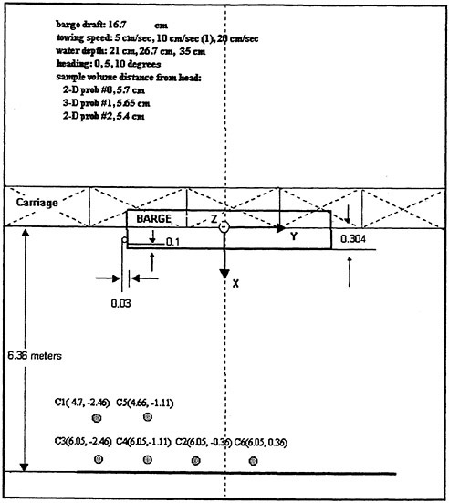
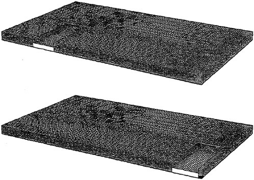
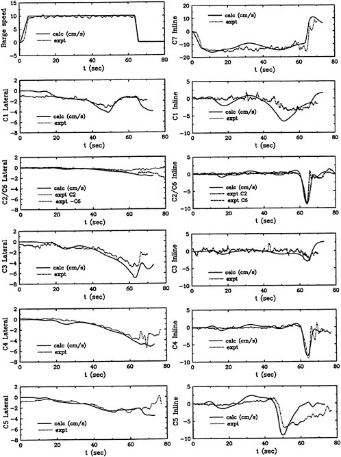
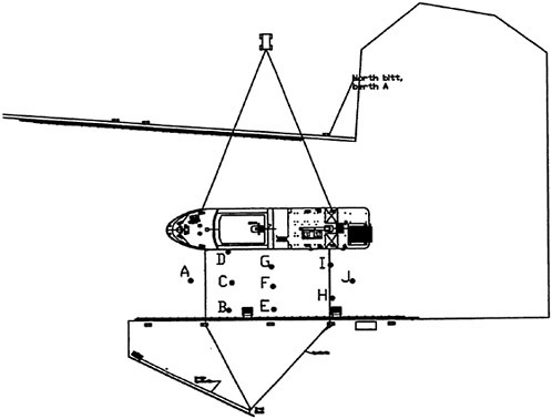
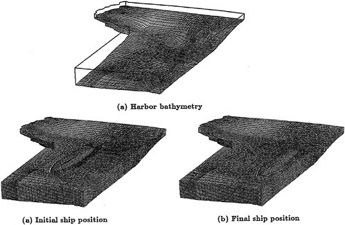
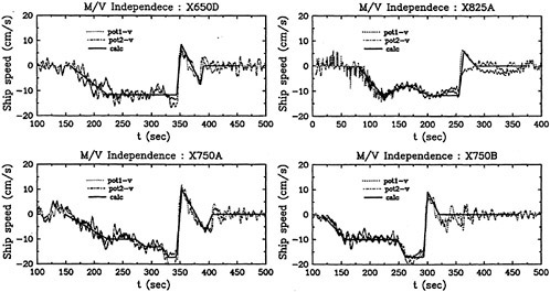
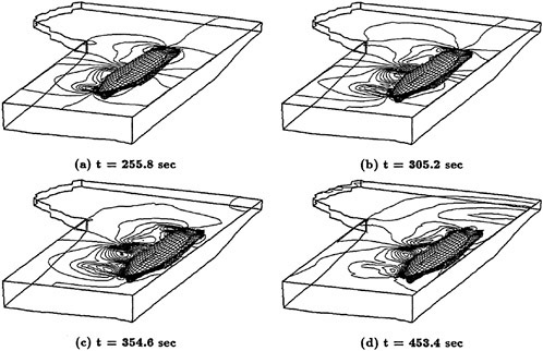
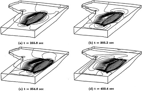
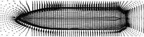
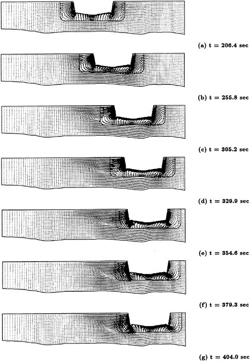
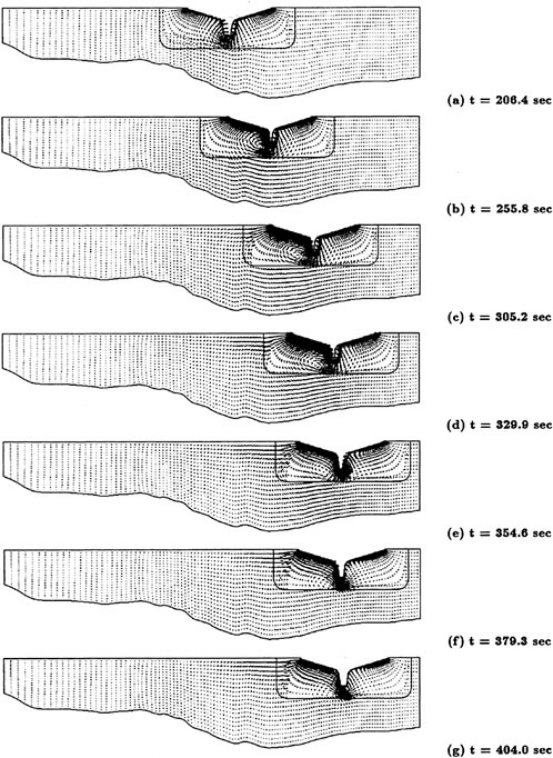
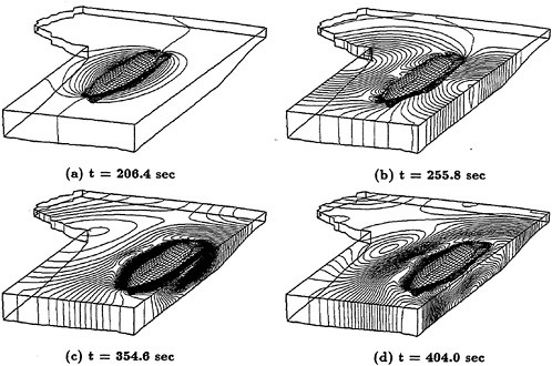
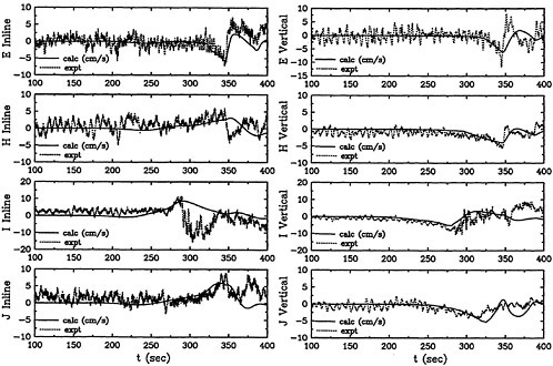
Validation of Free Surface Reynold’s Averaged Navier Stokes and Potential Flow Codes
T.Ratcliffe (Naval Surface Warfare Center, Carderock Division, USA)
The Office of Naval Research (ONR) has recently undertaken a Computational Fluid Dynamics (CFD) Validation Effort of Reynold’s Averaged Navier Stokes Codes (RANS) and Potential Flow Codes. These particular codes have been developed to predict the steady and unsteady hydrodynamic flow field around surface ships. Both types of codes have an important role in the ship design process. The potential flow codes are helpful in the initial hull form design process and can be run relatively quickly, allowing an assessment of bow and stern geometries over a range of speeds. RANS codes are more time-consuming to grid and run and therefore are best suited for use in flow analysis during the detailed ship design process.
An extensive set of validation data has been obtained on a combatant hull form, designated as DTMB Model 5415 and a standard series resistance model of Series 60. Experimental data obtained on these hull forms served as the basis for this CFD validation effort. Gathering of validation data is currently continuing with the addition of a geosym of Model 5415 built at Instituto Nazionale per Studi ed Esperienze di Architettura Navale (INSEAN) outside of Rome, Italy. This international collaboration will result in the most complete CFD validation effort on a naval combatant to date. In addition, overlapping data obtained in two different experimental facilities will be valuable in establishing the effect, if any, of different tow tank instrumentation and test procedures on the overall uncertainty of the experimental data.
DISCUSSION OF CODES
Both RANS codes and Potential Flow codes were part of this code validation effort. The RANS codes are CFDSHIP-IOWA, developed at the Iowa Institute of Hydraulic Research at the University of Iowa and UNCLE.OMAS, developed by the Engineering Research Center at Mississippi State University. The Potential Flow codes which were validated were: UMDELTA from the University of Michigan, SLAW and LAMP from SAIC, Annapolis and SWAN-1 from the Massachusetts Institute of Technology,
CFDSHIP-IOWA
CFDSHIP-IOWA is a generalized, multiblock RANS code for simulation of steady and unsteady free-surface flows around complex ship geometries. Exact non-linear kinematic and approximate dynamic free-surface boundary conditions are used to compute wave elevation on a computational grid that dynamically conforms to the free-surface wave elevation and hull geometry. Version 2.1 (V2.1) (1) of the code uses a finite analytic method for spatial discretization of the RANS equations and the PISO algorithm for the pressure-velocity coupling, while the latest version (V3.0) (2) improves accuracy and efficiency through the use of a higher-order upwind difference scheme for convection terms in the RANS equations. Both versions of the code use a higher-order upwind scheme for discretization of the convection terms in the kinematic free-surface boundary condition.
UNCLE.OMAS
UNCLE.OMAS is a time-accurate unsteady incompressible flow, RANS code, developed at the Engineering Research Center of Mississippi State University (3). The code is used for computations of the flow around surface ships, and includes the free surface. Currently, UNCLE.OMAS is based on the Modified Chorin’s Approach, where the modified continuity equation and momentum equation are of the same form as the equations without the body force potential, and the Froude number does not appear explicitly in the equations, only in the free surface boundary condition. This approach has advantages in that it results in a higher order resolution of the body force.
The characteristic variable boundary-conditions include inflow, outflow, impermeable and free surface boundaries. The numerical procedure uses a general, time dependent curvilinear coordinates in an implicit, upwind, finite volume approach. It has an unstructured multi-block capability and a multigrid capability. The solution is solved on dynamically deforming grid where the free surface is actually represented by a grid surface. Separate grids for tracking the free surface and for solving the bulk flow are not needed.
UMDELTA
UMDELTA (Desingularize Euler-Lagrange Time-Domain Approach) is a time-domain, fully nonlinear, potential flow code developed at the University of Michigan, to solve ship hydrodynamics problems (4,5). In UMDELTA, the fluid is assumed to be incompressible, inviscid and surface tension is neglected. A time-domain computational approach is used, and the ship hull is started from rest using the Euler-Lagrange approach. The method uses nonlinear free-surface boundary conditions to advance in time the position and potential of the free surface. The equations of mo-
tion of the body are used to advance in time the body boundary conditions applied on the wetted surface of the hull at an instant in time. The code is unique in it’s use of desingularized (isolated) Rankine sources. They are placed above the free surface, inside the body, and outside the bounding surfaces at infinity.
At present, the code has been successfully run on the Series 60 hull form. A geometry processor for transom-stern naval combatant hull forms has been completed and is currently being integrated into UMDELTA.
SLAW
SLAW is a Ship Lift and Wave free surface potential flow panel code, developed at SAIC, Annapolis (6). Either a Dawson-type or Rankine singularity model is employed to distribute source panels over a portion of the free surface, and a double-body linearization is applied at each panel. The body is modelled using a distribution of constant source panels or source plus doublets over the submerged portion of the hull. An upstream collocation shift is used to enforce the radiation condition on the free surface.
Velocities and pressures can be computed on the body, and forces and moments are computed by integrating the pressure on the hull surface. Sinkage and trim can be modeled automatically.
LAMP
LAMP is a Large Amplitude Motions Program for ship motion simulations and wave load predictions (7). The code was developed by SAIC in Annapolis. Large Amplitude Motions Theory involves the premises that there is likely to be large amplitude, mild-slope of the incident wave, and large amplitude ship motions, but small radiated and diffracted waves.
LAMP utilizes a time domain potential flow method with a wave resistance potential included to allow for sinkage and trim affects. This 3-D non-linear code includes forward speed and body/body interactions (for multi-hull geometries as well as multiple ships).
SWAN
SWAN-1 was also used for this validation effort The code was developed at the Massachusetts Institute of Technology (8,9). SWAN-1 is a ship-wave analysis program which is based on steady linearized free-surface potential flow theory. A boundary integral equation method is employed, using Green’s second identity. Rankine sources and dipoles are approximated by quadratic B-splines whose coefficients are obtained from a linear set of equations. This formulation requires the integral equation to be satisfied at collocation points on the hull and the mean free-surface level.
SWAN-1 allows the user to choose between free-stream linearization and double-body linearization. In the free-stream linearization scheme the end effects of the hull are not as well accounted for as they are in the double-body linearization.
VALIDATION DATA
Series 60
Series 60 was conceived in the 1950’s to establish a systematic series for the design of single screw merchant ships (10). The principal dimensions of the Series 60 model used in this study is shown in Table 1.
Table 1. Series 60 Model Principal Dimensions
|
Length |
3.048 m |
|
Beam |
0.406 m |
|
Draft |
0.163 m |
|
Displacement |
0.121 m3 |
|
Wetted Surface |
1.579 m2 |
|
Block Coefficient |
0.6 |
The model is made of FRP (fiber-reinforced fiberglass.) Only the unappended (bare hull) geometry has been used to obtain data for this validation effort. A representation of hull is shown in Figure 1.
Figure 1. Series 60 Model Lines
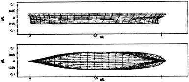
An extensive data set has been obtained on this model, both in the United States and abroad. The data which has been used for this validation effort was obtained at the University of Iowa, Iowa Institute of Hydraulic Research (IIHR) and consists of wave profiles along the hull, longitudinal wavecuts obtained at a fixed location away from the hull, stern wave height topography and velocity field measurements obtained at location of x/L=1.0, all at Fn=0.316. The bulk of the experimental data obtained at IIHR for the Series 60 is for the model in the free-to-sink-and-trim condition. Only the wave profiles along the hull were measured with the hull fixed at the design draft (11,12).
Wave Profiles
Wave profiles along the model were recorded for the model-fixed condition (at the design draft), using 35 mm and video photography.
Longitudinal Wavecuts
Wavecuts were obtained on this model using three capacitance wire probes whose position could be adjusted transversely in the basin. Data was obtained at 18 transverse locations and the y/L=.108 location was chosen for this validation effort.
Stern Topography
The local stern topography was mapped using a Shinozuka 15 cm AC servo-mechanism wave probe. An automated traverse was used to position the probe in a matrix of locations in the crossplane (y-z) direction relative to the model. The crossplane positioning was driven by two step motors controlled by a carriage-based microcomputer. Axial positioning was done by manually moving the y-z traverse system.
Velocity Field Measurements
A five-hole pitot probe (modified NPL type) was used to measure the direction and magnitude of the flow field in the plane x/L=1.0. The static side of a pitot-static tube measured the uniform stream pressure in undisturbed flow on the opposite side of the hull from the measurement plane.
The complete set of data is available at the following website: http:/iihr.uiowa.edu.
Model 5415
A surface combatant model, denoted as Model 5415, was the second of two models which was used to obtain validation data. The model was first tested in the 1980’s as part of a standard resistance and propulsion evaluation of this geometry and then more recently it was tested to gather specific data for code validation.
The model’s principal dimensions are shown in Table 2. For this validation effort only the bare hull (unappended) model was tested. A body plan and profile drawing of this model are shown in Figure 2.
Table 2. Model 5415 Principal Dimensions
|
Length |
5.72 m |
|
Beam |
0.76 m |
|
Draft |
0.248 m |
|
Displacement |
549 kg |
|
Wetted Surface |
4.83 sq. m. |
|
Block Coefficient |
0.506 |
Figure 2. Model 5415 Body Plane and Profile View
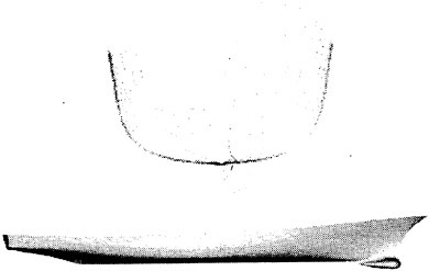
Validation data was obtained at the David Taylor Model Basin, Naval Surface Warfare Center, Carderock Division for two Froude numbers, Fn=0.28 and Fn=0.41. This validation study concentrated on the Fn=0.28 case and focused on the comparisons of wave profiles along the hull, longitudinal wave cuts obtained at a fixed distance from the hull, stern wave height topography, and velocity field measurements obtained in propeller plane (13,14).
All of the data collected for the Fn=0.28 case were obtained with the model fixed at the sinkage and trim for that speed. The sinkage of the forward and aft perpendiculars (FP and AP), relative to the even keel condition, is shown in Table 3.
Table 3. Model 5415 Sinkage Characteristics for Fn=0.28
|
Sinkage of FP |
Sinkage of AP |
|
−0.0021 L |
−0.0010 L |
|
(−) FP moves down |
(−) AP moves down |
|
(+) FP moves up |
(+) AP moves up |
Wave Profiles
Wave profiles were measured along the hull using a grease pencil and still photography. The wave profiles were recorded with reference to the design waterline drawn on the model, but this data was then converted to reference point z=0 at the undisturbed free surface using the known values for sinkage and trim.
Longitudinal Wavecuts
Longitudinal wavecuts were obtained on this model in two different ways. In the far field, a fixed capacitance wave probe was located at 1.854 m (y/L=0.324) from the centerline of the model. The fixed wave probes record the time history of waves generated by the model as it passes.
A second method of obtaining longitudinal wave cut records used stereophotography. Two calibrated “metric” cameras were mounted on ceiling-
mounted fixtures above the Carriage I Basin (15). As the model was towed down the basin, a sequence of photographs were taken, synchronized by strobe lights. The water surface was “seeded” using computer punch chips which were distributed on the surface before each run. Calibrated grid points in the far field, were imaged in the stereopairs and served as control points during the analysis of the photographs. The stereophotographs were measured by the National Ocean Survey and a digitized map of the free surface wave heights around the model was obtained. From this digital data, obtained at a resolution of 7.62 cm×7.62 cm, a longitudinal wave cut record was generated at y/L=0.097, providing near field wave elevation data along the model for the validation effort.
Stern Topography
A dynamic wave height “whisker” probe, similar to the servo-mechanism probe used at IOWA, was used to measure the surface topography in the stern region of Model 5415 as it was towed in the Carriage 2 Basin. The “whisker” probe uses a 2.54 cm long, 0.05 cm diameter, stainless steel needle to probe the water surface. The whisker is mounted on a vertical rod, attached to a servo motor. The whisker detects entry into the water by electrical conductivity; the water shorts out the small electrical potential on the whisker. Upon entry of the whisker into the water, the probe latches the analog output voltage representing this elevation and begins retracting the whisker probe. A traversing system using Thompson linear ball bearings for traverse rails was constructed. The traverse was automated in both the transverse and longitudinal directions and the location of the probe was obtained from the output of linear string potentiometers.
Velocity mapping in the propeller plane
Flow velocities were obtained in the propeller plane of Model 5415. The measurements were made using a five-hole pitot tube, with a 4.8 mm diameter hemispherical head. The probe was fitted to the base of a strut, which was attached to a two-axis traverse system mounted on the vertical rails of the Carriage 2 Basin. All velocity measurements were made in the propeller plane, at x/L=0.93. The resolution of the velocity grid was determined by obtaining predictions of the velocity gradients with both CFDSHIP-IOWA and UNCLE.OMAS, prior to the experiments. In a region close to the hull, the resolution was 0.0025 L. Farther out from the hull the spacing of the data was reduced to 0.005 L and then to 0.01 L.
The data is available at the following website: http://www50.dt.navy.mil/5415.
DISCUSSION OF COMPARISONS
Series 60
All the codes computed flow solutions for Series 60. The comparisons are shown in Figures 3 through 7. The computed longitudinal wavecuts and wave profiles along the hull, compared with the experimental results are presented in Figure 3. All the codes predict the phase of both the wavecut and the wave profile correctly. In the bow wave region, the RANS codes’ predictions show closer agreement to the experimental data than the potential flow codes. Insufficient paneling of the bow as well as the lack of adequate resolution of the radius of the bow at the waterline, could account for this deficiency in the potiential flow predictions.
Figures 4 and 5 show the stern flow topography for both the RANS codes and potential flow codes, respectively, as compared with the experimental results. The longitudinal location of the stern separation, the angle of the divergent stern wave with the hull, and the stern wave heights are well modeled in the RANS codes and in the potential flow codes with the exception of SWAN-1. The predictions obtained with SWAN-1 indicates that the code does not compute the angle of the divergent wave nor the wave elevations in the stern region correctly.
Figures 6 and 7 show comparisons of the axial velocity field and crossplane velocity vectors for Series 60. In these figures, the predictions from both RANS codes are compared to the experimental data. Both RANS codes accurately predict the width and depth of the wake deficit at x/L=1.0. The crossplane velocity vectors show the presence of a longitudinal vortex which is modeled in both predictions. The experimental data shows that the flow around the stern tube is still visible at this axial location, near the centerplane from z/L=−0.3 to z/L=−0.05. This feature is not well resolved in the RANS predictions.
Model 5415
Flow predictions were made on Model 5415 using the two RANS codes, CFDSHIP-IOWA and UNCLE.OMAS as well as SLAW, LAMP and SWAN-1. The other potential flow codes do not currently possess a robust method for modeling the transom stern geometry. The predictions are shown in Figures 8 through 12.
Figure 8 presents the comparisons of the predictions of a longitudinal wavecut and wave profile along the hull with experimental data for the naval combatant Model 5415. The bow wave is well predicted by both RANS codes, both on the hull and at the x/L=0.097 location. Both potential flow codes, SLAW and LAMP underpredict the bow wave on and off the body and underpredict the successive bow wave trough and shoulder wave crest at x/L=0.35. There is both phase and amplitude disagreement in the stern region of the longitudinal wavecut between the potential flow codes and the experimental wave height measurement. Increased panel resolution is likely to improve
the predictions from the potential flow codes of these hydrodynamic features.
Figures 9 and 10 show the stern surface topography predictions compared to the experimental measurements. In Figure 9 there is more difference in the stern region predictions between the RANS codes themselves than there have been in any of the other comparisons where RANS predictions have been made. There is a difficulty which both codes face, in generating a grid in the wake of a wetted transom stern. CFDSHIP-IOWA predicts a much reduced gradient of the stern waves along the centerline of the model than either UNCLE.OMAS or the experimental data. This could be due to the fact that the grid resolution is higher in the UNCLE.OMAS prediction than in the CFDSHIP-IOWA solution. In Figure 10, the SLAW and LAMP predictions are good, considering that these are potential flow predictions of such a complicated flow and do not include viscous effects. Both the angle of the divergent stern wave and the wave height contours are in reasonably good agreement with the experimental data, although the gradients in wave heights predicted by SLAW are larger along the centerline, aft of x/L=1.15, than the experiments document.
Figures 11 and 12 present the axial velocity contours and crossplane velocity vectors for the naval combatant, Model 5415. The plots clearly show a very different characteristic wake of this transom stern hull as compared to Series 60. Both RANS codes predict the transverse extent of the wake deficit. The only obvious difference in the two predictions is in 0.96 contour level of axial velocity. CFDSHIP-IOWA predicts a slightly deeper wake than either the UNCLE.OMAS predictions or the experimental data would indicate. The crossplane vector predictions are very similar to each other.
It is important to note that all code solutions were obtained at the institution where the code was developed. The results, therefore, represent extensive in-house expertise gained through experience with a particular code. It may also be significant to the comparison of the results that different grids and gridding techniques were used to obtain these solutions. Rigorous uncertainty assessments and grid resolutions studies need to be completed in order to fully assess these code comparisons.
FUTURE WORK PLANNED
This validation effort is continuing with work in progress at DTMB, IIHR, and INSEAN. At DTMB, Model 5415 will be appended with shafts and struts and the model will be fitted out with propellers and a torque and thrust dynamometer. In the fall of 1998, velocity measurements around one of the propellers will be obtained simultaneously with steady propeller torque and thrust measurements. In addition, the stern wave topography will be measured with the whisker probes to document the effect of propulsion on the stern wave system of the model. Finally, longitudinal wavecuts will be obtained with the propelled model. Validation data will be obtained on a geosym of Model 5415, at INSEAN. That work will focus on expanding the data set of off-body wave elevation measurements and obtaining velocity and pressure fields at a number of locations along the length of the model, including the x/L=0.93 location measured at DTMB. Collaborative work is also underway with IIHR. They are performing steady and unsteady hydrodynamics measurements on a small scale geosym of Model 5415.
ACKNOWLEDGMENTS
The author would like to thank Dr. Edwin Rood, Office of Naval Research, for the vision behind this validation effort and making the commitment to obtain high quality experimental data as part of the effort. In addition the author is indebted to Jennifer McDonald of Strategic Analysis, Inc. and Jim Rice at NSWC-CD who prepared most of the figures for this report.
REFERENCES
1. Paterson, E.G., Wilson, R.V., and Stern, F., “Verification/Validation for Steady Flow RANS Simulation of Model 5415,” 1st Symposium on Marine Applications of CFD, McLean, VA., 1998.
2. Wilson, R.V., Paterson, E.G., Stern, F. “Unsteady RANS for a Naval Combatant in Regular Head Waves,” ONR 22nd Symposium on Naval Hydrodynamics, Washington, D.C. August, 1988.
3. Beddhu, M. Jiang, Y., Whitfield, D.L, Taylor, L.K., and Arabshahi, A., “CFD Validation of the Free Surface Flow Around DTMB Model 5415 Using Reynolds Averaged Navier-Stokes Equations,” Third Osaka Colloquium on Advanced CFD Applications to Ship Flow and Hull Form Design, Osaka, Japan, May 25–27, 1998.
4. Scorpio, S.M., Beck, R.F., Korsmeyer, F.T., “Nonlinear water wave computations using a multipole accelerated, desingularized method”, 21st International Symposium on Naval Hydrodynamics, Trondheim, Norway, June, 1996, pp 64–74.
5. Beck, R.F., Cao, Y., Scorpio, S.M., Schultz, W., “Nonlinear ship motion computations using the desingularized method”, 20th International Symposium Naval Hydrodynamics, Santa Barbara, Calf., August, 1994, pp 227–246.
6. Weems, K.M., Lin, W-M., and Chen, H.C., “SLAW Ship Flow Calculations Using Inviscid and
Interactive Zonal Viscous Approaches,” Ship Research Institute CFD 94, Tokyo, 1994.
7. Lin, W-M., Weems, K., Zhang, S. and Treakle, T., “Steady and Unsteady Ship Waves Predicted by Large-Amplitude Motion Program,” 1st Symposium on Marine Applications of Computational Fluid Dynamics, McLean, Virginia, USA, 1998.
8. Sclavounos, P.D., Kring, D.C., Huang, Y-F, Mantzaris, A., Kim, S. and Kim, Y. “A Computational Method as an Advanced Tool of Ship Hydrodynamic Design”. Proc. SNAME 97 Annual Meeting, 1997, Ottawa, Canada.
9. Sclavounos, P.D. and Huang, Y-F. “Rudder Winglets on Sailing Yachts”, Marine Technology, July 1997.
10. Todd, F.H., “Series 60 Methodical Experiments with Models of Single-Screw Merchant Ships”, DTMB Report 1712, 1963, David Taylor Model Basin, Bethesda, MD
11. Toda, Y., Stern, F., Longo, J., “Mean-Flow Measurements in the Boundary Layer and Wake and Wave Field of a Series 60 CB=0.6 Ship Model-Part 1: Froude Numbers 0.16 and 0.316,” J. Ship Research, Vol. 36, No. 4, 1992, pp. 360–377.
12. Longo, J., Stern, F., and Toda, Y., “Mean-Flow Measurements in the Boundary Layer and Wake and Wave Field of a Series 60 CB=0.6 Ship Model-Part 2; Scale Effects on Near-Field Wave Patterns and Comparisons with Inviscid Theory,” J. Ship Research, Vol. 37, No. 1, 1993, pp. 16–24.
13. Ratcliffe, T., Mutnick, I., Rice, J., McGuigan, S., “Bow and Stern Wave Height Topography around Model 5415”, August, 1998, CRDKNSWC/HD-1478–02, Naval Surface Warfare Center, Carderock Division, West Bethesda, MD.
14. Ratcliffe, T., Mutnick, I., Rice, J., “Velocity Field Measurements in the Propeller Plane of Model 5415”, August, 1998, CRDKNSWC/HD-1478–01, Naval Surface Warfare Center, Carderock Division, West Bethesda, MD.
15. Ratcliffe, T., Lindenmuth, W., “Kelvin Wake Measurements on Five Surface Ship Models,” January 1980, DTRC-89–038, David Taylor Research Center, Bethesda, MD.
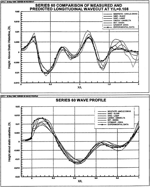
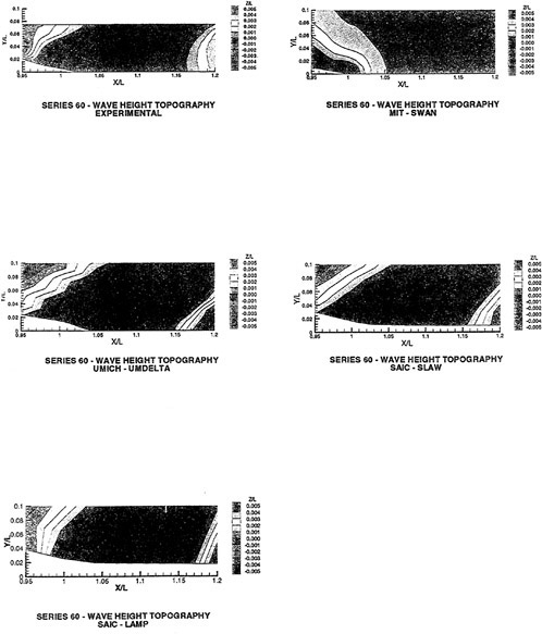
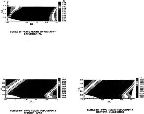
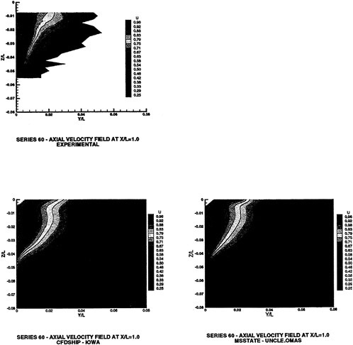
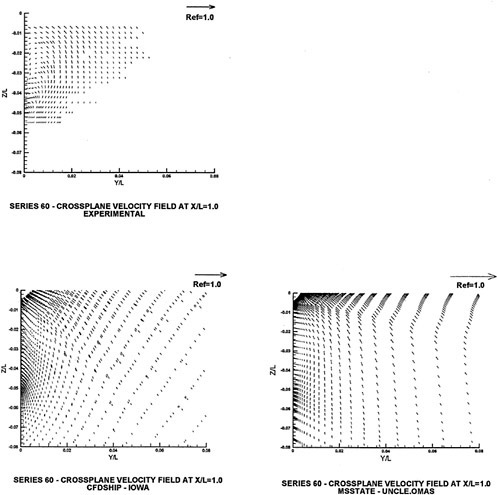
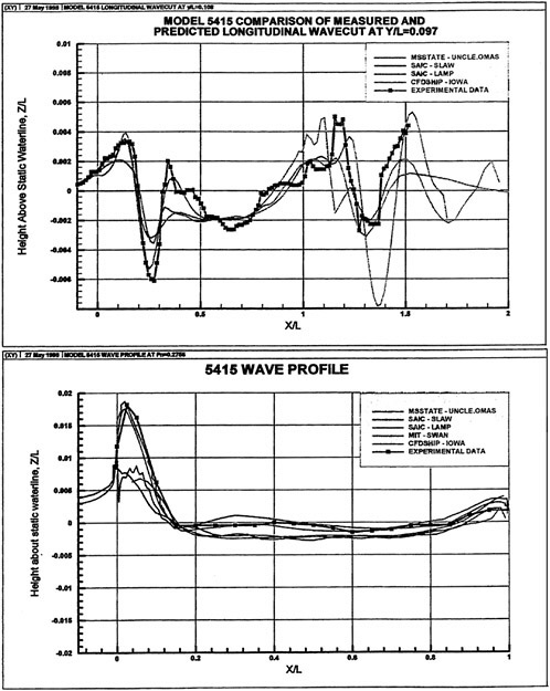
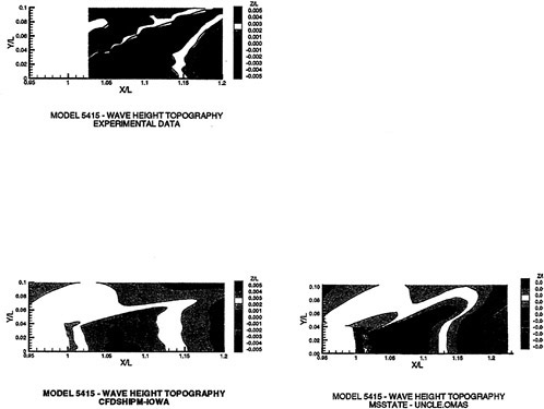
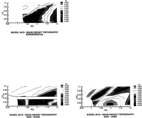
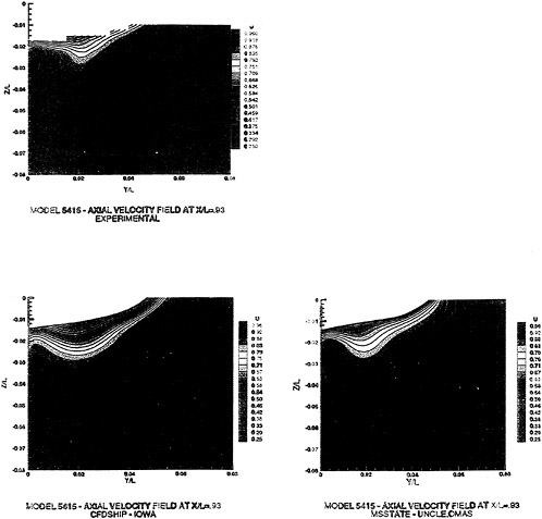
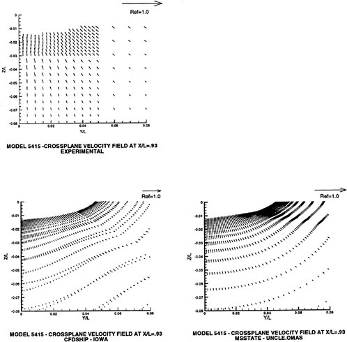
DISCUSSION
H.Haussling
Naval Surface Warfare Center, Carderock Division, USA
The author has done an excellent job of comparing measured data with computational predictions. The results for Model 5415 are particularly notable because of the challenge of both measuring and computing the flow field for such a transom stern hull. It is discouraging to see, in Figure 9, such a large difference between the two RANS predictions of the stern wave pattern. It is mentioned that a possible explanation is the relative coarseness of the grid in the CFDSHIP-IOWA computation. It is surprising that this hypothesis has not yet been tested. It is to be hoped that a computation can soon be carried out with a refined grid to ascertain whether inadequate grid resolution or something else is the reason for the difference. If the explanation is more complex, and if it turns out to be difficult to determine for this challenging recirculating flow problem, it might be worthwhile to consider the higher speed case (Froude no.=0.41). This is a simpler flow, with dry transom, treated compu-tationally with promising results at David Taylor Model Basin [1]. Application of the RANS codes to this less challenging problem might help sort out remaining unknowns affecting stern wave predictions.
Reference
[1] “Computation of High-Speed turbulent Flow about a Ship Model with a Transom Stern,” by H.J.Haussling, R.W.Miller, and R.M. Coleman, Naval Surface Warfare Center, Carderock Division Report CRDKNSWC/ HD-0200–51, Sept. 1997.
AUTHOR’S REPLY
The author thanks Mr. Haussling for his discussion of this paper, and for including the reference to his computations on the Model 5415 hullform. Mr. Haussling’s concern regarding the CFDSHIP-IOWA solution for Model 5415 stern topography is well-founded and the code developers at the University of Iowa have undertaken an effort to compute new solutions for that Froude No.=0.28. Grid resolution was increased in the transom stern region and resulted in an improved resolution of the peak value in the stern wave behind the model. These results are presented in Paterson et al. (1998).
The predictions initially presented in the preprints from this ONR conference were obtained using CFDSHIP-IOWA, Version 2.1. During the last few months, stern wave topography solutions were obtained using a new version of the code, Version 3.0. Figure 1 shows a comparison of the two solutions. As described in the text of this paper, Version 3.0 has improved accuracy and efficiency over the earlier version due to the use of higher-order upwind differencing scheme for the convection terms in the RANS equations. The Version 3.0 solution is shown, compared to the experimental data in Figure 2. The improvements in the resolution of the details of the stern wave topography, in particular the region of highest elevations, are attributed to the decreased numerical dissipation in the higher-order upwind scheme used in Version 3.0 code.
The author again thanks Mr. Haussling for his discussion and looks forward to future dialogue in the coming year as more validation data is made available to the computational community.
Reference
Paterson, E.G., Wilson, R.V., and Stern, F., (1998), “Verification/Validation for Steady Flow RANS Simulation of the Model 5415,” 1st Symposium on Marine Applications of CFD, McLean, VA.
Comparison of CFD and EFD for the Series 60 CB=0.6 in Steady Yaw Motion
Y.Tahara,1 J.Longo,2 F.Stern,2 Y.Himeno1
(1Osaka Prefecture University, Japan, 2University of Iowa, USA)
ABSTRACT
This paper presents comparisons of computational and experimental fluid dynamics results for boundary layers and wakes and wave fields of the Series 60 CB=0.6 ship model in steady yaw motion. The numerical method solves the unsteady Reynolds-averaged Navier-Stokes and continuity equations with the Baldwin-Lomax turbulence model, exact nonlinear kinematic and approximate dynamic free-surface boundary conditions, and a body/free-surface conforming grid. The experimental and computational conditions, i.e., Froude number 0.16 and 0.316 for the experiments and 0 and 0.316 for the computations, allow comparisons of low and high Froude number results, respectively, which enables evaluation of Froude number effects and validation of the computational fluid dynamics at both low and high Froude number. Satisfactory agreement is demonstrated between the calculations and the experimental data, which supports the conclusion that the present approach can accurately predict ship boundary layers and wakes, including free-surface effects for the yawed case. In the following, an overview is given of the present numerical approach, and the computational conditions and uncertainty analysis are described. Results are presented for the wave and flow fields with emphasis on the important flow features of yaw-and wave-induced effects in comparison with the experiments. Finally, conclusions from the present study are given with recommendations for future work.
NOMENCLATURE
|
Β |
ship beam |
|
CB |
block coefficient (=∇/(LBT)) |
|
Cp |
|
|
Fr |
|
|
g |
gravitational constant |
|
H |
|
|
L |
characteristic (ship) length |
|
n |
normal direction; time level |
|
n |
normal unit vector |
|
p |
static pressure; order of accuracy |
|
|
piezometric pressure |
|
r |
radial coordinate; grid-refinement ratio |
|
Re |
Reynolds number (=UoL/ν) |
|
Sb, Se, etc. |
boundaries of the solution domain |
|
T |
ship draft |
|
U, V, W |
mean velocity components |
|
UE, UD, etc. |
uncertainties |
|
Uo |
characteristic (freestream) velocity |
|
Uτ |
|
|
X, Y, Z |
Cartesian coordinates |
|
Y+ |
dimensionless distances (=ReUτYn) |
|
Yn |
distance normal to the wall surface |
|
β |
yaw angle |
|
|
sampled variables or integrals |
|
ν |
kinematic viscosity |
|
νt |
eddy viscosity |
|
ρ |
density |
|
τw |
wall shear stress |
|
ωx |
axial vorticity |
|
ξ, η, ζ |
body-fitted coordinates |
|
ζ |
free-surface elevation, residuals |
|
∇ |
ship displacement |
INTRODUCTION
Although the yaw condition is an approximation to the maneuvering ship condition [1], it involves many features of interest that must be accurately evaluated for hull form design, e.g., asymmetric wave and flow patterns, breaking waves and breaking-wave wakes, wave- and body-induced vortices, spray, and bubble entrainment [2, 3]. In contrast to the straight-ahead (zero-yaw) condition, the yaw condition is dominated by strong crossflow effects, including forebody and afterbody keel and bilge vortices. The distinct vorticity in the flow field originates from strong yaw-induced crossflow and large crossplane
pressure gradients. For the high-Froude number (Fr) case, wave-induced effects on the boundary layer and wake are significant due to the larger wave amplitudes especially on the windward side than for the zero-yaw case.
Recent advancements in computational fluid dynamics (CFD) enable application of Reynolds-averaged Navier-Stokes (RANS) equation methods to the present problem [4–10]; however in most cases, the wave effects are not considered in the theory, where the free surface is treated as a symmetry plane. On the other hand, considerable effort has been focused on development of the RANS equation method for calculating viscous free-surface flows, and the recent status of CFD in ship hydrodynamics is such that the steady resistance and flow for the zero-yaw case are nearly at the accuracy of the experimental data, although certain issues for further improvements are involved [11]. Nevertheless, relatively little attention has been given to the extension of the RANS equation methods so as to consider free-surface effects for the yaw condition. This may be due to the difficulties in simulation of the complicated free-surface flow features, e.g., those mentioned above, considerably higher computational load than that required for the zero-yaw condition, and more importantly, limited information from experimental fluid dynamics (EFD) to enable detailed evaluation and validation of the CFD results.
In the present study, a large-domain approach of [12] is applied to the problem with extensions for application to the steady yaw condition. The RANS and continuity equations are solved with the Baldwin-Lomax turbulence model, exact nonlinear kinematic and approximate dynamic free-surface boundary conditions, and a body/free-surface conforming grid. The results are evaluated through comparisons with recently completed extensive EFD results for the Series 60 CB=0.6 ship model at low (0.160) and high (0.316) Fr for yaw angle (β)=10° [3]. The former case essentially simulates the zero-Fr condition such that the comparisons with the latter case enables the identification of salient features of the wave-induced effects. In [12], results for zero yaw angle and similar comparisons were presented for the same geometry with detailed experimental data of [13, 14]. Due to the limitation of numerical treatment of the free-surface boundary conditions, breaking-wave and bubble entrainment effects will not be discussed in detail in this paper.
In the following, an overview is given of the present numerical approach, computational conditions, and numerical uncertainty analysis. The results are presented for wave and flow fields with emphasis on important flow features of yaw- and wave-induced effects and comparisons with experiments. Finally, conclusions from the present study are given with recommendations for future work.
COMPUTATIONAL METHOD
The computational method is basically the large-domain approach of [12] for steady straight-ahead condition. Some extensions are made to include both sides of the ship hull in consideration of the yaw condition. The large-domain approach [12] is based on extensions and modifications of the interactive approach in [15, 16]. Additional information on the numerical approach is provided in [17] including transition for design applications, including extensions for naval combatants with bulbous bows and transom sterns, utilizing multi-block domain decomposition and propeller-hull interaction, utilizing the method of [18]. Herein, an overview is given.
The numerical method solves the unsteady RANS and continuity equations for mean-velocity (U, V, W) piezometric pressure ![]() and eddy viscosity νt by using the Baldwin-Lomax turbulence model, exact nonlinear kinematic and approximate dynamic free-surface boundary conditions, and a body/free-surface conforming grid. The equations are transformed from Cartesian coordinates (Χ, Υ, Ζ) in the physical domain to numerically-generated, boundary-fitted, nonorthogonal, curvilinear coordinates (ξ, η, ζ) in the computational domain. A partial transformation is used, i.e., coordinates but not velocity components (U, V, W). The equations are solved using a regular grid, finite-analytic spatial and first-order backward difference temporal discretization, PISO-type pressure algorithm, and the method of lines. For steady-flow application, time serves as a convergence parameter and the grid is updated at each time step to conform to both the body and free surface.
and eddy viscosity νt by using the Baldwin-Lomax turbulence model, exact nonlinear kinematic and approximate dynamic free-surface boundary conditions, and a body/free-surface conforming grid. The equations are transformed from Cartesian coordinates (Χ, Υ, Ζ) in the physical domain to numerically-generated, boundary-fitted, nonorthogonal, curvilinear coordinates (ξ, η, ζ) in the computational domain. A partial transformation is used, i.e., coordinates but not velocity components (U, V, W). The equations are solved using a regular grid, finite-analytic spatial and first-order backward difference temporal discretization, PISO-type pressure algorithm, and the method of lines. For steady-flow application, time serves as a convergence parameter and the grid is updated at each time step to conform to both the body and free surface.
As shown in Figure 1, consider a ship fixed in the uniform onset flow Uo=(Uocosβ, Uosinβ, 0), where β is yaw angle. Take the Cartesian coordinate system with the origin on the undisturbed free surface, X and Υ axes on the horizontal plane, and Ζ axis directed vertically upward. Figure 1 also shows the solution domain. For application to the present yaw condition, the solution domain includes both port and starboard sides of the hull. Referring to Figure 1, the specified boundaries are the body surface Sb, the inlet plane Si, the exit plane Se, the outer boundary So, and the free-surface Sζ which for zero Fr becomes the symmetry waterplane Sw. The boundary
conditions for zero Fr are: on Sb, ![]()
![]() (where n is normal to the body); on Si, freestream values are imposed, i.e., U=Uocosβ, V=Uosinβ,
(where n is normal to the body); on Si, freestream values are imposed, i.e., U=Uocosβ, V=Uosinβ, ![]() on Se, axial diffusion and pressure gradient are assumed negligible, i.e.,
on Se, axial diffusion and pressure gradient are assumed negligible, i.e., ![]()
![]() and on So, U=Uocosβ, V=Uosinβ,
and on So, U=Uocosβ, V=Uosinβ, ![]() (where n is normal to the surface). For nonzero Fr, the boundary conditions are similar, except on Sζ, where exact nonlinear kinematic and approximated dynamic free-surface conditions are applied on the exact free surface, which is determined as part of the solution; i.e., the dynamic conditions ∂(U, V, W)/∂Z=0 and
(where n is normal to the surface). For nonzero Fr, the boundary conditions are similar, except on Sζ, where exact nonlinear kinematic and approximated dynamic free-surface conditions are applied on the exact free surface, which is determined as part of the solution; i.e., the dynamic conditions ∂(U, V, W)/∂Z=0 and ![]() are applied to velocity and pressure with ζ determined through the solution of the exact nonlinear kinematic condition using a Beam and Warming linear multi-step scheme with both explicit and implicit 4th-order artificial dissipation and local time stepping based on the local velocity magnitude. The boundary conditions for ζ are: on Si, ζ=0; on S0, ∂ζ/∂η=0; and on Se, ∂ζ/∂Χ=0.
are applied to velocity and pressure with ζ determined through the solution of the exact nonlinear kinematic condition using a Beam and Warming linear multi-step scheme with both explicit and implicit 4th-order artificial dissipation and local time stepping based on the local velocity magnitude. The boundary conditions for ζ are: on Si, ζ=0; on S0, ∂ζ/∂η=0; and on Se, ∂ζ/∂Χ=0.
The RANS grid is Η-type with constant-X planes stacked to form a complete three-dimensional grid. The bow and stern are resolved by axial clustering of grid points distributed with hyperbolic tangent stretching functions. Because of the H-type grid, non-vertical sterns are resolved in a staircase fashion. The constant-X cross-plane grids are generated elliptically by solving a Poisson equation for the transformation between (Υ, Ζ) and (η, ζ). Spacings are specified in the η-direction at the surface of the hull, which for the Baldwin-Lomax turbulence model should be at a Y+≈1, and in the ζ-direction at both the centerplane and free surface. The initial grid must extend to an elevation sufficiently above the zero, or design waterline, to allow for wave crests. As the wave field develops, the RANS grid conforms to the free surface. By conforming the grid points and saving the initial distribution along η=constant, or girth-wise lines, the grid is easily updated; the point on the free surface moves to a new elevation and all points below the free surface slide along the η=constant line so as to maintain the initial relative distribution.
The kinematic free-surface boundary condition grid, which is independently generated from the RANS grid, is two-dimensional (i.e., a function of X and Y), updated iteratively to fit the wave-hull intersection, and it is different from the RANS grid in that, instead of high near-wall resolution, more points are distributed in the outer flow to resolve the wave field. The grid is 460×200 to include both sides of the hull and consists of equal spacing in the axial direction and a power distribution in the transverse direction. Communication between the RANS and free-surface grid is accomplished using bi-linear interpolation such that the velocity field from the ζ=1 and kp1 (minimum and maximum indices of grids in ζ-direction, correspond to port- and starboard-side free surfaces, respectively) plane is interpolated to the free-surface grid. Similarly, the wave elevation is interpolated from the free-surface grid to the ζ=1 and kpl plane of the RANS grid. See [12] or [17] for more details of the present numerical method.
EXPERIMENTAL DATA AND COMPUTATIONAL CONDITIONS AND GRIDS
Recently, extensive EFD results were obtained for the Series 60 CB=0.6 ship model in steady yaw motion at the Iowa Institute of Hydraulic Research [3]. The data includes: photographs and video; resistance, side force, and yaw moment; sinkage, trim, and heel angle; wave profiles along the hull and wave elevations; and mean-velocity and pressure fields for numerous crossplanes from the bow to the near wake. In the study, detailed descriptions are provided of the experimental equipment, procedures, and uncertainty analysis. The Series 60 CB=0.6 ship model is a single-propeller merchant-type ship, a standard for ship-hydrodynamics research, and in particular, was chosen with three other hull types as a representative hull form for the Cooperative Experimental Program (CEP) [19].
The conditions simulate the experiments; i.e., Uo=1; L=1; and for low Fr, Fr=0 and Re=2.00×10⁶, and for high Fr, Fr=0.316 and Re=4.00×10⁶, although the experimental Re is somewhat different, i.e., average Re=2.50×10⁶ and 4.93×10⁶ for low and high Fr, respectively. Note that the experimental low-Fr case is defined as Fr=0.16; however, free-surface effects are relatively small, except near the bow. A partial view of the Fr=0.316 RANS grid is shown in Figure 2. For both Fr, the inlet, exit, and outer boundaries are located at X=(−0.4 and 2.0) and r=1, respectively. The first grid points off the body surface are located in the range Y+<2 (=ReUτYn). The RANS grids are prepared as follows: for Fr=0, 90×40×60=216,000 (Grid A), 90×60× 60=324,000 (Grid B), 90×80×60=432,000 (Grid C), and 108×48×72=373,248 (Grid D) (in longitudinal×radial×girthwise directions); and for Fr=0.316, 180×40×80=576,000 (Grid E), 180× 60×80=864,000 (Grid F), and 180×80× 80=1,152,000 (Grid G). The free-surface boundary condition grid size is 460×200=92,000 for both port and starboard side free surface for all Fr=0.316 grids. The values of the time increment and
underrelaxation factors for velocity and pressure are 0.01, 1, and 0.1 for Fr=0, and 0.01, 1, and 0.01 for Fr=0.316. The computations are completed for 40 and 80 non-dimensional timesteps for Fr=0 and 0.316, respectively, although the convergence criterion is satisfied earlier, such that the residual defined by equation (31) in [12] for all variables be about 10−4, which is satisfied in 20 and 40 nondimensional timesteps for Fr=0 and 0.316, respectively. The computed hydrodynamic forces indicate small oscillations with minimal reduction in the residuals after the above-mentioned convergence criterion is satisfied. This may be due to iterative nonconvergence, or possibly due to the unsteady nature of the flow involving three-dimensional flow separation associated with unsteady vortex shedding. The oscillation of the solutions is considered in the analysis of iteration uncertainty described in the following section.
UNCERTAINTY ANALYSIS
In the following, more detailed characteristics of the present computational grids are discussed in conjunction with uncertainty analysis. The numerical uncertainty analysis should include iterative and grid convergence tests and possibly order-of-accuracy studies. Note that the derivation of the finite-analytic method precludes term-by-term error analysis and that equation error depends on both cell Re and aspect ratio. Order-of-accuracy studies on the present finite-analytic method is carried out in [17, 20] for both simple and practical geometries, in which it is stated that order-of-accuracies vary between about 1.5–2.5 depending on geometry and flow complexity. The verification procedure of the present results basically follow that in [17], however, validation processes described in [21] are also needed, and are currently in progress.
In [21], comparison error is defined as the resultant of all errors associated with the data and all errors associated with the simulation and is written as the difference, E=D−S. The uncertainty UE, in the comparison error is defined as: UE2=UD2+US2, where UD and US are experimental and simulation uncertainties, respectively. US can be written as: US2=USN2+USPD2+USMA2, where USN simulation numerical uncertainty, USPD uncertainty based on sensitivity analysis of model coefficients, and USMA model assumption. Hence, validation uncertainty UV defined as UV2=UE2−USMA2=UD2+USN2+USPD2 is key metric in the validation process. In the present study, USPD is ignored, and USN in [21] is evaluated by USN2=USG2+USI2, where USG=3ε/(rP−1), ![]() in percent or for relative expression,
in percent or for relative expression, ![]() and
and ![]() variables or integral values for finer and coarser grids, r grid refinement ratio, and p order of accuracy. USI is iterative convergence uncertainty, whose estimation is based on evaluation of the iteration records of integral and point variables. The level of the iterative convergence is determined by the number of orders of magnitude reduction and magnitude in the residuals
variables or integral values for finer and coarser grids, r grid refinement ratio, and p order of accuracy. USI is iterative convergence uncertainty, whose estimation is based on evaluation of the iteration records of integral and point variables. The level of the iterative convergence is determined by the number of orders of magnitude reduction and magnitude in the residuals ![]() where n is the iteration number and
where n is the iteration number and ![]() can either be the solution variables or equation imbalances obtained by back substitution. For simple geometries and flows, sixteen orders of magnitude reduction of ζ to machine zero is possible such that the iterative convergence uncertainty is negligible. However, for practical geometries and flows, only a few orders of magnitude reduction in ζ to about 10−4 may actually be attainable. In this case, the estimates for iterative convergence uncertainty are based on statistics of the iteration records of integral and point variables and taken as roughly one-half the difference between the maximum and minimum values.
can either be the solution variables or equation imbalances obtained by back substitution. For simple geometries and flows, sixteen orders of magnitude reduction of ζ to machine zero is possible such that the iterative convergence uncertainty is negligible. However, for practical geometries and flows, only a few orders of magnitude reduction in ζ to about 10−4 may actually be attainable. In this case, the estimates for iterative convergence uncertainty are based on statistics of the iteration records of integral and point variables and taken as roughly one-half the difference between the maximum and minimum values.
Table 1 provides forces and moment of the present results for Fr=0 and 0.316, and the grid convergence is evaluated in Table 2. For Fr=0, grid increase in radial direction, i.e., grids (A), (B), and (C), show oscillatory ε for lift and convergent ε for drag and moment. However, only one directional analysis may result in underestimation of grid convergence characteristics. In grid (D), numbers of points of grid (A) are increased in all directions, i.e., the total number of points is about 1.7 times as large as that of grid (A), and the ε between the two grids appears to be more realistic. For Fr=0.316, only one directional analysis is done, and similarly as for Fr=0, show convergent ε for lift and oscillatory ε for drag and moment. In Table 3, the above-mentioned numerical uncertainties are shown, including resultant validation uncertainty UV, where UD is given by EFD results of [3]. In analysis of USG, assumed p=1.5 is used, and ε evaluated between grids (A) and (D), and (E) and (G) is used for Fr=0 and 0.316, respectively. The value of USG for Fr=0.316 are based on only radial-directional analysis, i.e., that is denoted as USGη, is likely underestimated USG to result in underestimation of UV, since USG is defined as summation of the values in all direction, i.e., U2SG=U2SGξ+U2SGη+U2SGζ. The USI is evaluated based on one-half the difference between the maximum and minimum values of the iteration records for last 10 non-dimensional time, for which solutions for grids (D) and (G) are used for Fr=0 and 0.316, respectively. Note that as the number of total grid points increases, the USI tends to be larger. The sampling of point values of velocity and pressure fields are made at a
point in the near wake region, i.e., (X, Y, Z)=(1, 0, −T), where Τ is the maximum draft of the hull. Better alternative of the sampling point may be in the region near the core of keel or bilge vortices; however, difficulties occurs in interpolation may preclude accurate estimation of the uncertainties, and in fact, the location of the vortex core slightly changes as the computational grid changes.
In summary, for Fr=0, evaluated numerical uncertainties USN are about 2% to 5% for hydrodynamic forces, 1% to 4% for mean-flow solutions, and validation uncertainties UV are about 5% to 8% for hydrodynamic forces, and 2% to 4% for mean-flow solutions. On the other hand, USN for Fr=0.316 are as follows: about 1% to 3% for hydrodynamic forces; about 3% for wave profiles; about 4% for wave elevations; and about 1% to 4% for mean-flow solutions. UV for Fr=0.316 are as follows: about 1% to 3% for hydrodynamic forces; about 4% for wave profiles; about 4% for wave elevations; and about 2% to 5% for mean-flow solutions. Further detailed uncertainty analysis for the present results is currently in progress.
RESULTS
In the following, results are presented and discussed for Fr=0 and 0.316, including comparison with experimental data. In general, the emphasis of the discussions concerns the comparisons and evaluation of the computational method, whereas reference is made where appropriate to [3] for relevant discussion and interpretation of the flow physics; however, in some cases, for clarity of presentation, certain discussions are replicated. The discussions include comparison between zero-(β=0°) and nonzero-(β=10°) yaw angle results, although in some cases, the former is not shown in the present figures. See [12] for details of β=0° solutions including comparisons with experimental data of [13, 14].
Integral variables
First, integral variables are discussed. Table 1 shows comparison of the forces and moment of the present results. It must be noted that the sinkage and trim are all fixed in the present computation but free in the measurements, which preclude quantitative comparison between the two results. Therefore, the comparison is focused on the trend between high and low Fr. As indicated in Table 1, the differences between Fr=0.316 (grid G) and 0 (grid D) for CL, CD, and CMz are roughly (−6%, −21%, −17%) in magnitude, and those for experiments between high (0.316) and low (0.16) Fr are roughly (−16%, −26%, −39%), i.e., the same trends are predicted by the present method. The differences between the present and experimental data can likely be attributed to the above-mentioned differences in the fix/free condition. In addition, some shortcomings of the present method in resolving complicated features in flow field may be related to the differences, e.g., underpredicted magnitude of axial vortices as well as absence of wave-breaking and bubble-entrainment effects. Those are discussed later in conjunction with comparison of the computational results with the experimental data.
Surface pressure and frictional streamlines
Next, surface-pressure distributions are considered. The surface-pressure and axial and vertical surface-pressure gradient contours for β=10° and Fr=0 and 0.316 are shown in Figure 3. Unfortunately, no experimental data are available for comparison. Significant differences are observed between the present and precursory β=0° [12] results. The differences are mainly due to increase and decrease of pressure in port and starboard sides, respectively, which correspond to the pressure and suction sides, respectively. Also, differences between Fr=0 and 0.316 are clearly displayed, which is due to the nonlinear free-surface effects for the latter. Figure 4 shows computed frictional streamlines for β=10° and Fr=0 and 0.316. For Fr=0.316, flow patterns correlate with the pressure and pressure gradient displayed in Figure 3. On the forebody port side, a pocket of low pressure region is observed near the bilge, which causes the flow to converge towards the keel, and partially converges at the keel and separates to generate forebody-keel vortex. On the forebody starboard side, streamlines are downward and towards the bilge and meet the streamlines from forebody port side, and finally the streamlines form an open-type three-dimensional separation pattern, that is related to generation of forebody-bilge vortex. A closed-type separation region is also seen near the bow on the starboard side. On the other hand, on the afterbody starboard side, low pressure region is located near the stern bilge, which causes the streamlines to converge towards the stern bilge, and meet the streamlines from port side and finally form the open-type separation pattern, which results in generation of afterbody-bilge vortex. Streamlines on afterbody portside partially converge at the keel and separate to generate afterbody-keel vortex. Similar aspects of frictional streamlines are displayed for Fr=0; however in this case, free-surface effects are absent and the differences are obvious especially near the waterline. In addition for Fr=0, the larger region of closed-type separation is observed near the bow on starboard side than for Fr=0.316.
Wave profiles
The wave profile at the hull is compared with the experimental data in Figure 5. The results for both port and starboard sides demonstrate fairly close agreement with the measurements with respect to wave amplitude, shape, and phase, although some systematic differences are observed. The amplitudes of port-side bow-wave crest and trough are somewhat underpredicted. Similarly, on the starboard side, wave amplitudes are slightly underpredicted on the forebody. Some underprediction displayed near the bow on the starboard side is likely related to limitations of the present numerical method, i.e., although experiments observed flow separation associated with wave-breaking in this region, that is not completely reproduced in the present method. For both sides of the hull, good agreement is observed after X=0.5, although some details on the starboard side around X=0.9 are not completely predicted.
The trends and differences between β=0° and 10° are well reproduced in the present computations (i.e., the most resulting changes to the profiles (Δζ) occur upstream of X=0.25; for X<0.25 the port-side profile shifts upward significantly with increases in β, and the largest increase in profiles occur where ζx=0; the starboard-side profile decreases significantly with increase in β, and again, the largest Δζ occurs where ζx=0; for X>0.25, the influence of β is fairly small except for decreases and increases in the fore and aft shoulder-wave troughs).
Wave elevations
Figure 6 shows contours of the wave elevations and axial wave slopes for Fr=0.316 and β=0° [12] and 10°. Similar trends and differences between β=0° and 10° are displayed between the present results and the measurements, i.e., the wave amplitudes clearly increase on the port side and decrease on the starboard side of the model with increasing β, and for β=10°, similarly with β=0°, ζx is in phase with ζ and has similar patterns, but the magnitudes are significantly increased and decreased globally on the port and starboard sides, respectively. For β=10°, the wave patterns become asymmetrical, and the computed elevations show close similarity with the experimental data with regard to both amplitude and shape for the forebody, i.e., experimental ζx indicates that the port bow-wave crestline curves back towards the model with increasing X, and a similar trend is observed in the present results. However, in the global region in the starboard side, the bow wave system propagation downstream is not very clearly reproduced. The results for the afterbody also show fairly close similarity; but the detailed resolution particularly of the complex global-region wave system in the starboard side is incomplete. The differences between the present and experimental results increases as distance from the hull increases, which is likely due to the decrease of computational grid density in the region.
Mean velocity and pressure field
Finally, results for the mean-velocity and pressure field are presented in Figures 7 through 10. Figures 7 and 8, and 9 and 10 show results for Fr=0 and 0.316, respectively, and Figures 8 and 10 are from the experimental results of [3]. Contours of ωx, H, and Cp are shown at the same crossplanes as those of the measurements, i.e., X=(0, 0.1, 0.2, 0.4, 0.6, 0.8, 0.9, 1.0, 1.1, 1.2). For both the present and experimental results, the overall trends are similar between the Fr=0 and 0.316 flow fields, in which significant free-surface effects are also exhibited for the latter. Most of the flow features in the yawed condition are significantly different from those for zero-yaw case. In many respects, the flow is completely altered. The boundary-layer and wake development is dominated by strong crossflow effects and vortices as opposed to axial pressure gradients and weak crossflow effects observed in the β=0° case. The wave-induced effects at Fr=0.316 are explainable similarly as for β=0°, i.e., the Fr-related differences in the velocity and pressure correlate with the wave field, which, however, is significantly more complex for β=10° than for β=0° creating a more complex boundary-layer and wake response. In the following, more details are discussed
Figures 9a and 10a compare the axial vorticity contours for Fr=0.316. For both experimental and computational results, the extensive vorticity (ωx) in the flow field is evident. Note that the contour ranges for the present and experimental results are different, i.e., −20<ωx<20 and −50<ωx<50 for the former and latter, respectively. In the present results, magnitudes of ωx are generally underpredicted, although many important aspects of the vortices near the hull are well reproduced in the present results (i.e., on the forebody, keel and bilge vortices are visible beginning at X=0.1, where the keel vortex is relatively weak and not evident beyond X=0.4, and the bilge vortex is relatively strong; the vortex core is off the body and moves further from the centerplane with increasing x; and on the afterbody, the forebody-bilge vortex weakens, and an afterbody-bilge vortex develops as per β=0°, where the vorticity has a core region that is off of the body and toward the free surface with a tail that extends toward the centerplane,
and there appears to be a weak interaction with the forebody-bilge vortex). In the present results, the forebody-bilge vortex weakens faster than that for measurements, which is likely due to the inadequate accuracy in turbulence model and longitudinal grid resolution. In the region near the stern, the present results indicate quite a few similarities with the measurements, e.g., a counter rotating keel vortex is evident at X=1 after perpendicular (AP), although the magnitude is somewhat underpredicted. The important flow aspects in the wake region are also similar between the present and experimental results (i.e., the forebody-bilge vortex dissipates and diffuse with trajectory towards the free surface, where the afterbody-bilge vortex becomes oval shaped and dissipates and diffuses with a trajectory off the body towards the free surface; and the afterbody-keel vortex dissipates relatively fast with a trajectory as per the afterbody-bilge vortex, and there is limited interaction between fore- and afterbody-bilge vortices). In the experimental data, a wave-induced vortex is evident on the port-side forebody which initiates between 0.2<X<0.4 underneath the breaking bow wave and follows a trajectory near the free surface along the side of the hull. Although the present free-surface boundary conditions do not include exact breaking wave effects, similar wave-induced vortex is reproduced in the region; but the magnitude is somewhat reduced.
Figures 7a and 8a compare the axial vorticity contours for low Fr, i.e., Fr=0 and 0.16 for the present and experimental results, respectively. In the measurements, the overall flow pattern is similar to that of Fr=0.316 but with two important differences as follows: the bilge and keel vortices appear weaker, and the trajectories are altered somewhat; and due to the reduced wave field, there is no wave-induced vorticity in the flow field. The similar trend of the differences between low and high Fr are displayed in the present results; but also, the shortcomings discussed for Fr=0.316 hold true for Fr=0. In addition, some wave-induced effects on flow field are observed in the measurements especially in the region near the bow on the port side, although the influences are much smaller than those for Fr=0.316.
In Figures 7b through 10b, the total head (H) field is presented, where the viscous regions (H) on the hull and in the wake are compared between the present results and measurements. In the experimental data for Fr=0.316, the patterns correlate with ωx and the boundary layer and wake losses but with stronger interactions than for low Fr between the loss regions of the keel and bilge vortices on the afterbody creating a somewhat more complex pattern. The flow aspects observed in the measurements are well reproduced in the present results, although some details in the near wake are not complete. For both results, Η displays similar Fr differences as per ωx for the wave-induced vortex, i.e., for Fr=0.16, in contrast with ωx which decreased in magnitude with decreasing Fr, Η is somewhat increased in magnitude which is a Reynolds number effect, i.e., the viscous regions are thicker for the lower Fr.
Lastly, the pressure field is considered. In Figures 7c through 10c, the present and measured pressure (Cp) field around the hull is displayed. In general, the present results indicate many similarities with the measurements (i.e., at the forebody for Fr=0.316, Cp correlates with U such that the trends are the same but the magnitudes are reversed especially in the bow and stern regions and at the midbody where the flow accelerates and the pressure is low; an asymmetric stagnation-type flow is exhibited at the forward perpendicular (FP); generally, high and low pressure regions exists on the port and starboard sides, respectively; the lowest pressures are in regions of high ωx with minimums in the core regions; and the bow wave stagnation effects are evident as increased pressures at X=0 and 0.1). In both results for Fr=0.316, the pressure differences (ΔCp) between port and starboard sides are reduced near the midbody at X=0.4, and at the afterbody, there is a continued reduction in Δp up to X=0.9 when ΔCp increases with the lowest Cp in regions of high ωx and minimums in the core regions, i.e., for the forebody-bilge vortex and afterbody-bilge vortex. It appears in both results that, apparently, most of the sideforce is generated near the bow and somewhat near the stern where ΔCp is largest. For Fr=0, the present results indicate that the general patterns are similar to those for Fr=0.316 except for some diminished features due to Fr and viscous effects (i.e., the pressure at the bow and stern is lower due to the reduced port-side bow wave system and wave effects at the AP and wake, respectively; and the pressure field is higher over the midbody and stern especially in the regions of the vortex cores), and the similar trends are observed in the experimental data. As described above, many important features in the measurements are successfully simulated in the present method; however, some details related to magnitude of longitudinal vortices are not complete, which can be attributed to the earlier-mentioned shortcomings, i.e., insufficient turbulence model and grid resolution.
SUMMARY AND CONCLUSIONS
This paper presents comparison of CFD and EFD for boundary layers and wakes and wave fields around practical three-dimensional geometry of the Series 60 CB=0.6 ship model in steady yaw motion. The numerical method solves the unsteady RANS and continuity equations with the Baldwin-Lomax turbulence model, exact nonlinear kinematic and approximate dynamic free-surface boundary conditions, and a body/free-surface conforming grid. EFD results from towing tank experiments at both low (0.16) and high (0.316) Froude number are used for the comparison, in which the former case essentially simulates the zero Froude number condition such that the comparisons with the latter case enables the identification of the salient features of the wave-induced effects. In addition, comparison of the results with those from an earlier study for the straight-ahead condition enables investigation of yaw-and wave-induced effects. Discussion of the results are focused on important flow features of yaw- and wave-induced effects in comparison with experiments.
Satisfactory agreement is demonstrated between the calculations and the experimental data, i.e., the asymmetric wave field close to the hull, and mean-flow fields dominated by strong crossflow effects that drive the flow from the port to the starboard side and asymmetric vorticity development at the forebody bilge, forebody keel, afterbody bilge, and afterbody keel are correctly simulated. In addition, trends between low and high Fr for integral variables and mean-flow fields indicate good agreement with the measurements. However, complex details regarding vortex generation and evolution are somewhat underestimated in magnitude, and amplitudes in the global-region wave field are underpredicted and bow-wave system for starboard side are not completely reproduced in the global region. The issues for the wave fields are similar to that of the precursory work for zero-yaw condition [12], which may be because no particular improvement is done on the numerical technique in this study. The same holds true for the issues regarding resolution of vortices, i.e., the turbulence model and numerical scheme are same as those of [12], and longitudinal grid density is also similar to that used in [12]. Although results obtained by the present method are promising, further improvement must be made on the above-mentioned in order to solve the problem. In addition, inclusion of breaking-wave and bubble entrainment effects are important to more accurately simulate the flow in yaw condition. Furthermore, more complete numerical uncertainty analysis is needed in conjunction with more detailed grid convergence study especially for non-zero Fr condition.
ACKNOWLEDGEMENTS
This research was sponsored by the Office of Naval Research under Contract N00014–96–0018 including allocation for super computing hours at DOD HPC resources (NAVO T90), both of which are under the administration of Dr. E.P.Rood whose support is greatly appreciated. Also, this research was supported by the Japan-U.S. Cooperative Science Program of National Foundation of Science of U.S.A. under Contract INT-9513138 and Japan Society for The Promotion of Science. The authors’ thanks are extended to whom concerns the program for their kind support and encouragement.
REFERENCES
1. Day, W.G. and Hurwitz, R.B., (1980), “Propeller-disk wake survey data for model 4989 representing the FF 1055-class ship in a turn and with a bass dynamometer boat,” Report no. SPD-0011–21, David Taylor Naval Research and Development Center, Bethesda, MD.
2. Longo J. and Stern, F., (1995), “Evaluation of surface-ship resistance and propulsion model-scale database for CFD validation,” J. Ship Research, Vol. 40, No. 2, pp. 112–116.
3. Longo J. and Stern, F., (1996), “Yaw effects on model-scale ship flow,” Proc. the 21st Symposium on Naval Hydrodynamics, June 25, 1996, Trondheim, Norway.
4. Tahara, Y., (1995), “Computation of Boundary-Layer and Wake Flows around IACC Sailing Yacht,” J. Kansai Society of Naval Architects, Japan, No. 224, pp. 1–11.
5. Tahara, Y., (1996), “A Multi-Domain Method for Calculating Boundary-Layer and Wake Flows around IACC Sailing Yacht,” J. Kansai Society of Naval Architects, Japan, No. 226, pp. 63–76.
6. Ohmori, T. and Miyata, H., (1993), “Oblique Tow Simulation by a Finite-Volume Method,” J. Society of Naval Architects of Japan, Vol. 173, pp. 27–34.
7. Ohmori, T., Fujino, M., Miyata, H., Kanai, M., (1994), “A Study on Flow Field Around Full Ship Forms in Maneuvering Motion—1st Report: In Oblique Tow-,” J. Society of Naval Architects of Japan, Vol. 176, pp. 241–250.
8. Ohmori, T., Fujino, M., Tatsumi, K., Kawamura, T. and Miyata, H., (1996), “A Study on Flow Field Around Full Ship Forms in Maneuvering Motion—3rd Report: Flow Field Around Ship’s Hull in Steady Turning Condition-,” J. Society of Naval
Architects of Japan, Vol. 179, pp. 125–138.
9. Akimoto, H., Hiroshima, F. and Miyata, H., (1996), “Hydrodynamic Design of a Sailing Boat by CAD/CFD System with Moving Coordinates,” Proc. 3rd Korea-Japan Joint Workshop on Ship & Marine Hydrodynamics, Taejon, Korea
10. Campana, E.F., Di Mascio, A. and Penna, R., (1998), “CFD Analysis of the Flow Past a Ship in Steady Drift Motion,” to appear Proc. 3rd Osaka Colloquium on Advanced CFD Applications to Ship Flow and Hull Form Design, Osaka, Japan
11. CFD Tokyo Workshop, (1994), Tokyo, Japan
12. Tahara Y. and Stern, F., (1996), “A Large-Domain Approach for Calculating Ship Boundary Layers and Wakes for Nonzero Froude Number,” J. Computational Physics, Vol. 127, 1996, pp. 398–411.
13. Toda, Y., Stern, F. and Longo, J., (1992), “Mean-Flow Measurements in the Boundary Layer and Wake and Wave Field of a Series 60 CB=0.6 Ship Model—Part 1: Froude Numbers .16 and .316,” J. of Ship Research, Vol. 37, No. 4, pp. 360–377.
14. Longo, J., Stern, F. and Toda, Y., (1993), “Mean-Flow Measurements in the Boundary Layer and Wake and Wave Field of a Series 60 CB=0.6 Ship Model—Part 2: Scale Effects on Near-Field Wave Patterns and Comparisons with Inviscid Theory,” J. of Ship Research, Vol. 37, No. 1, pp. 16–24.
15. Tahara, Y., Stern, F. and Rosen, B., (1992), “An Interactive Approach for Calculating Ship Boundary Layers and Wakes for Nonzero Froude Number,” J. Computational Physics, Vol. 98., No. 1, pp. 33–53.
16. Tahara Y. and Stern, F., (1994), “Validation of an Interactive Approach for Calculating Ship Boundary Layers and Wakes for Nonzero Froude Number,” J. Computers and Fluids, Vol. 23, No. 6, pp. 785–816.
17. Stern, F., Paterson, E.G. and Tahara, Y. (1995), “CFDSHIP-IOWA: Computational Fluid Dynamics Method for Surface-Ship Boundary Layers, Wakes, and Wave Fields,” IIHR Report, No. 381, Iowa Institute of Hydraulic Research, Iowa City, IA 52242, USA.
18. Stern, F., Kim, H.T., Zhang, D.H., Toda, Y., Kerwin, J. and Jessup, S. (1994), “Computation of Viscous Flow Around Propeller-Body Configurations: Series 60 CB=0.6 Ship Model,” J. Ship Research, Vol. 38, No. 2, pp. 137–157.
19. ITTC, (1987), “Report of the Resistance and Flow Committee,” Proc. 18th Int. Towing Tank Conference, Kobe, Japan, pp. 47–92.
20. Zhang, Z.J. and Stern, F., (1996), “Free-Surface Wave-Induced Separation,” ASME Journal of Fluids Engineering, Vol. 118, pp. 546–554.
21. Coleman, H.W. and Stern F., (1998), “Uncertainties and CFD Code Validation,” to appear J. Fluids Engineering.
Table 1. Lift, drag, and moment.
|
Conditions |
Fr=0,β=10° Re=2×10⁶ |
Fr=0.316,β=10° Re=4×10⁶ |
|||||
|
Grid |
90×40×60 |
90×60×60 |
90×80×60 |
108×48×72 |
180×40×80 |
180×60×80 |
180×80×80 |
|
Lift (CL=L/.5ρSDWLU02) |
1.826E-02 |
1.837E-02 |
1.836E-02 |
1.792E-02 |
1.870Ε-02 |
1.891E-02 |
1.898E-02 |
|
(%CL) hydrostatic (z/Fr2) |
0.00% |
0.00% |
0.00% |
0.00% |
−23.46% |
−23.46% |
−23.46% |
|
(%CL) piezometric (p hat) |
102.25% |
102.19% |
102.21% |
102.21% |
125.56% |
125.48% |
125.45% |
|
(%CL) frictional |
−2.25% |
−2.19% |
−2.21% |
−2.21% |
−2.10% |
−2.02% |
−1.99% |
|
Drag (CD=D/.5ρSDWLU02) |
8.445E-03 |
8.406E-03 |
8.381E-03 |
8.298E-03 |
1.043E-02 |
1.047E-02 |
1.046E-02 |
|
(%CD) hydrostatic (z/Fr2) |
0.00% |
0.00% |
0.00% |
0.00% |
−7.53% |
−7.53% |
−7.53% |
|
(%CD) piezometric (p hat) |
51.50% |
52.40% |
52.40% |
50.40% |
71.08% |
71.94% |
72.47% |
|
(%CD) frictional |
48.50% |
47.60% |
47.60% |
49.60% |
36.45% |
35.59% |
35.06% |
|
Moment (CMz=Mz/.5ρLpp3U02) |
−1.186E-03 |
−1.188E-03 |
−1.190E-03 |
−1.174E-03 |
−1.408E-03 |
−1.408E-03 |
−1.408Ε-03 |
Table 2. Grid convergence.
|
Conditions |
Fr=0.β=10° Re=2×10⁶ |
Fr=0.316,β=10° Re=4×10⁶ |
|||||
|
Grid |
(A) 90×40×60 |
(B) 90×60×60 |
(C) 90×80×60 |
(D) 108×48×72 |
(E) 180×40×80 |
(F) 180×60×80 |
(G) 180×80×80 |
|
ε: Lift (CL=L/.5ρSDWLU02) |
|
0.58% |
−0.01% |
−1.91% |
|
1.10% |
0.39% |
|
ε: Drag (CD=D/.5ρSDWLU02) |
−0.47% |
−0.30% |
−1.78% |
0.36% |
−0.07% |
||
|
ε: Moment (CMz=Mz/.5ρLpp3U02) |
0.17% |
0.11% |
−1.01% |
−0.02% |
0.01% |
||
|
Evaluation of ε |
Bet.(A)–(B) |
Bet.(B)–(C) |
Bet.(A)–(D) |
Bet.(E)–(F) |
Bet.(F)–(G) |
||
Table 3. Summary of numerical and experimental uncertainties.
|
Conditions |
Fr=0,β=10° Re=2×10⁶ |
Fr=0.316,β=10° Re=4×10⁶ |
||||||||
|
|
USG (%) |
USI (%) |
USN (%) |
UD (%) |
UV (%) |
USGη(%) |
USI (%) |
USN (%) |
UD (%) |
UV (%) |
|
Lift (CL) |
4.9 |
0.4 |
4.9 |
1.8 |
5.2 |
2.4 |
0.3 |
2.5 |
0.1 |
2.5 |
|
Drag (CD) |
4.6 |
0.2 |
4.6 |
6.0 |
7.5 |
0.5 |
0.5 |
0.7 |
0.6 |
0.9 |
|
Moment (CMz) |
2.4 |
0.4 |
2.4 |
4.1 |
4.8 |
0.5 |
0.3 |
0.6 |
0.1 |
0.6 |
|
Wave Profiles |
- |
- |
- |
2.6 |
- |
3.2 |
0.6 |
3.2 |
1.3 |
3.5 |
|
Wave Elevations |
- |
- |
- |
2.2 |
- |
4.0 |
0.6 |
4.0 |
1.1 |
4.2 |
|
Mean Flow |
|
|||||||||
|
U (%U0) |
3.9 |
0.7 |
4.0 |
1.5 |
4.3 |
1.2 |
0.8 |
1.4 |
1.5 |
2.1 |
|
V (%U0) |
2.7 |
0.7 |
2.8 |
1.5 |
3.2 |
1.2 |
0.8 |
1.4 |
1.5 |
2.1 |
|
W (%U0) |
0.2 |
0.7 |
0.7 |
1.5 |
1.7 |
0.2 |
0.8 |
0.8 |
1.5 |
1.7 |
|
Cp |
0.1 |
0.4 |
0.5 |
3.0 |
3.0 |
3.5 |
0.6 |
3.6 |
3.0 |
4.7 |
|
- : Not applicable or negligible |
||||||||||
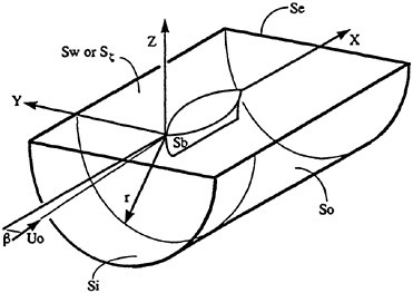
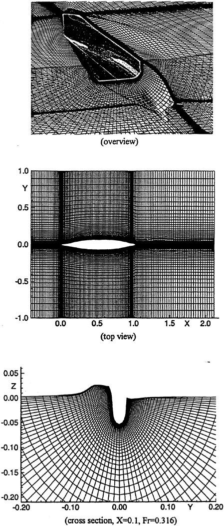
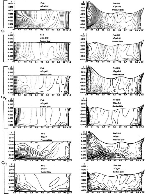
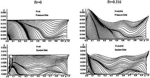
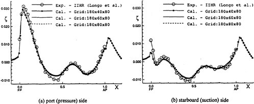
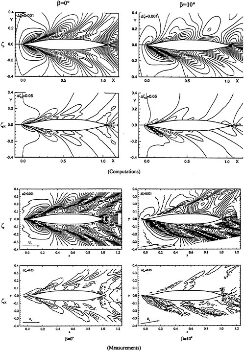
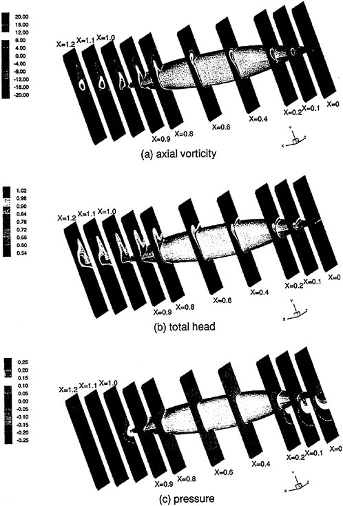
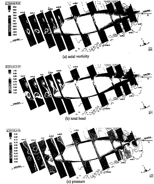
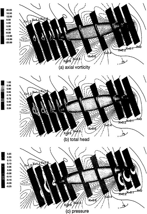
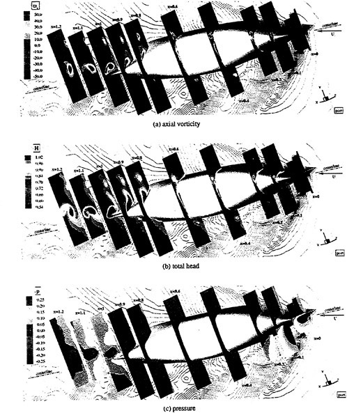
DISCUSSION
U.Bulgarelli
Istituto Nazionale per Studi ed Esperienze di Architettura Navale, Italy
Thank you for a very interesting presentation. In one of your transparencies you mentioned a local time stepping. Could you say some words on how to compute that local step?
AUTHORS’ REPLY
The local time stepping we used can be interpreted as normalization of free-surface kinematic boundary condition (FSKBC) using the magnitude of local flow velocity. Velocity magnitude in the near wall region is very small, such that integration of FSKBC to obtain free-surface elevation tends to be unstable near the wall surface. As far as steady solution is considered, the present method appears to provide sufficient solution accuracy and numerical stability, which have been demonstrated in the application to other types of ship hull, e.g., the naval combatant.
DISCUSSION
Τ.Suzuki
Osaka University, Japan
Thank you for your excellent presentation. I have a question about stern flow field around the model ship. We, Osaka University group, measured flow field around a series 60, CB z 0.6 model by triple hot wire anemometry in wind tunnel.
We compared six components of Reynolds stress distributions with several turbulence models. In that case, even if the velocity distributions have good agreement between CFD and EFD, the Reynolds stress distributions do not agree so much.
The question is, did you compare the Reynolds stress distributions as well as velocity distributions? If not, please compare them to validate CFD codes in this stage. I think, from a physical point of view, it is very important to compare the stress distributions.
AUTHORS’ REPLY
We have not completed evaluation of prediction accuracy in Reynolds-stress fields of the present results, which is mainly due to the fact that the experimental data obtained by Longo et al. did not include the information. I agree with your point stating that turbulent quantity as well as mean-velocity fields must be predicted accurately in order to investigate underlying flow physics related to the present problem. We are planning to consider further evaluation and validation of the present method, in association with consideration of more advanced turbulence models. We highly appreciate your experimental data, and will set forth more critical evaluation of the present results.
The Scaling of High Reynolds Number Viscous Flow Predictions for Appended Submarine Geometries
P.Bull, S.Watson (Defence Evaluation and Research Agency, United Kingdom)
Introduction
The flow around typical marine vessels has several features which must be correctly accounted for in order to allow accurate flow predictions. These flow features include the development of the hull boundary layer, flow separation, flow into and through the propulsor, vortices formed at the root and tip of appendages and several more. All of these features combine and interact to produce a very complex, turbulent, three-dimensional flow field.
Whilst the fluid flow can be measured by using a scale model of the vessel in a towing tank or wind tunnel, there are errors associated with applying results obtained at model scale to full scale vessels. Furthermore, experiments of this type require many detailed measurements to be taken in the regions of interest. This is costly and time consuming.
Computational Fluid Dynamics (CFD) has been shown to be capable of predicting the fluid velocity distributions at model scale to accuracies of around 5% of measured values, but many of these predictions have failed to capture accurately details of the flow features, for example, the wake harmonics [1].
The size, strength and position of the flow features is generally dependent on the density and viscosity of the fluid, the length of the vessel, and the speed and direction of the vessel through the fluid. Therefore, the flow around model scale vessels differs from the flow around the equivalent full scale vessel because these flow features vary with the length and speed of the vessel. Such scaling is characterised by the non-dimensional Reynolds’ number which changes from values of order 106–107 at model scale to values of order 108–109 for full scale. In general, as the Reynolds’ number increases, the flow features become more compact and compressed, and the boundary layers and shear layers get thinner in relation to the length of the vessel.
Recent advances in CFD, especially in the field of turbulence modelling, have been developed which have been shown to be capable of predicting flow at full scale Reynolds’ numbers [2,3,4]. This paper describes the application of such turbulence models to the aft section of submarine ‘like’ geometries over a range of Reynolds’ numbers. The particular geometries are the SUBOFF AFF1 and AFF4 configurations, for which detailed flow measurements are available at model scale for comparison with numerical predictions.
Governing Equations
The governing equations which describe the motion of a viscous, incompressible fluid are Navier Stokes equations and the equation of continuity. These fundamental equations are averaged over a period of time to produce the Reynolds’ Averaged Navier Stokes (RANS) equations. This averaging process introduces the Reynolds’ stresses which require a turbulence model to provide closure. A number of different turbulence models, with various levels of complexity have been examined over recent years. Standard two-equation turbulence models, such as RNG k-ε, have been widely used to examine the flow at model scale but have not been used routinely for predictions of the full scale flow. More recently, the Wilcox and Menter k-ω models and various Reynolds’ stress models have been shown to provide better comparison with measured data for a typical tanker hull [5,6,7].
©British Crown copyright. Reproduced with the permission of the Controller of Her Majesty’s Stationery Office. The views expressed are those of the authors and do not necessarily reflect the views or policy of the Ministry of Defence, Her Majesty’s Stationery Office, or any other British government department
The accurate prediction of flows over a range of Reynolds’ numbers requires a model for the turbulent length scales which accounts for the changes in Reynolds’ number. Such scaling is especially important in the thin shear layers, regions with high pressure gradients and regions with strong flow curvature.
This paper describes some preliminary CFD results of the Reynolds’ scaling of the RNG k-ε and the standard Wilcox and the Menter k-ω turbulence models in the presence of an adverse pressure gradient and with embedded vortices in the boundary layer.
The incompressible RANS equations for momentum and continuity are:
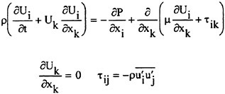
These equations are closed by a model for the turbulent Reynolds stresses.
The standard RNG k-ε turbulence model for the turbulent kinetic energy k and the dissipation rate ε, with a linear relationship between stress and strain is:
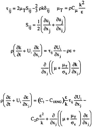
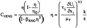
where
The Wilcox turbulence model replaces the equation for ε with the ω equation where:
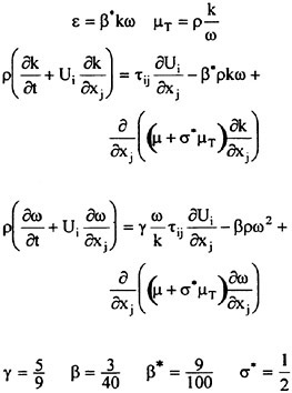
The Menter variant of the k-ω turbulence model blends the ω equation between the Wilcox model near walls and the standard k-ε model
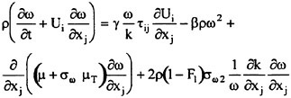
where the constants are weighted between the two limiting cases:
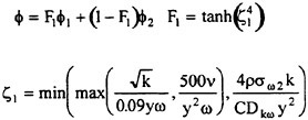
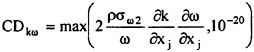
κ=0.41 β*=0.09 y=distance from wall
The coefficients for the two cases are given below in table 1.
Table 1
Coefficients for Wilcox and Menter turbulence models
|
|
|
|
|
σk |
0.5 |
1.0 |
|
σω |
0.5 |
0.856 |
|
β1 |
0.0750 |
0.0828 |
|
γ |
|
|
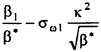

Initial and Boundary Conditions
The boundary conditions for the wall play an important role in the evaluation of near wall flows. The standard RNG k-ε uses a ‘wall function’ to prescribe the behaviour of the near wall flow, whereas the Wilcox and Menter models solve the system of equations ‘down to the wall’.
The inlet and initial conditions were defined in non-dimensional terms such that:
x=non dimensional distance along the body

The mean velocity profile at the inlet boundary is characterised by the required Reynolds’ number, given by
The wall function approach assumes a logarithmic form of the viscous layer
where
and E=9.81
The parameters used to define the required initial profile were:
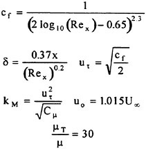
For y>δ
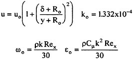
For y<δ, the velocity and turbulence profile are defined in three distinct ranges
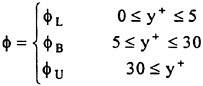
for ![]() and ω respectively. The axial velocity is prescribed by
and ω respectively. The axial velocity is prescribed by
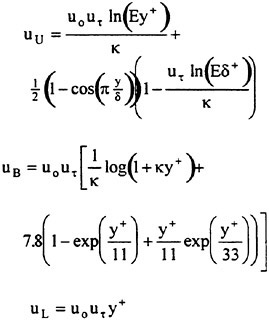
turbulent kinetic energy by
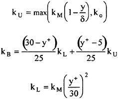
and ω by
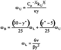
The initial values for epsilon were defined for y+>50 from k and ω when appropriate.
The profiles for the turbulence parameters at the inlet plane were subsequently modified from their upstream values to ensure that the inlet profile satisfied equilibrium conditions within the boundary layer.
Grid Generation
In order to generate suitable grids for the computation of flows using these turbulence models it is necessary to use a fast efficient grid generation system. The system must be capable of producing high quality grids with sufficient grid density to resolve the flow parameters. The system used was the SAUNA system, produced for DERA by the Aircraft Research Association. This system uses the elliptic multi-block method to generate grids around appended geometries.
The turbulence models outlined above place particular requirements on the grid generation. The most critical of these is the requirement to control the distance of the first cells from the wall. This distance can be defined in terms of y+, the non-dimensional spacing. The different turbulence models have different requirements for this spacing as given in table 2. The grids suitable for the Wilcox and Menter models had cell spacings which give y+=1.0 and the grids for RNG k-ε had cell spacings for y+=50.0.
Table 2
First Cell Spacing for Different Reynolds’ Numbers
|
Reynolds Number |
cf ×103 |
uτ ×102 |
y+ |
Cell Spacing |
|
1.2×10⁷ |
2.787 |
3.733 |
1.0 50.0 |
2.232×10⁻⁶ 1.116×10⁻⁴ |
|
1.2×10⁸ |
2.001 |
3.163 |
1.0 50.0 |
2.635×10⁻⁷ 1.317×10⁻⁵ |
|
1.2×10⁹ |
1.500 |
2.737 |
1.0 50.0 |
3.045×10⁻⁸ 1.525×10⁻⁶ |
This table highlights the difficulties associated with the generation of grids for full scale submarines. The first cell spacing is several orders of magnitude smaller than a representative length scale for the submarine. This requires a smooth definition of the geometry surface.
In addition to the spacing of the first cell layer from the wall, it is necessary to consider the support for the flow gradients in the thin shear layers. To obtain reasonable grid support through the viscous sub-layer, the number of grid layers is substantially larger for turbulence models with no wall function. Typically, 10–20 cells are required in the boundary layer with wall functions and 30–50 cells are required without. It is also necessary to ensure that the pressure gradients are adequately resolved.
These requirements mean that additional care must be taken within the grid generation process to ensure that accurate, high quality grids are produced within the boundary layers. The total number of cells required to ensure this quality increases for the advanced turbulence models. A grid for a fully appended submarine, suitable for standard turbulence models requires approximately 1–2,000,000 cells whereas a grid suitable for advanced turbulence models with equivalent resolution of the pressure gradients requires 3–5,000,000 cells.
Improvements to the SAUNA multi-block grid generation system, have enabled the rapid
generation of grids suitable for full scale flow calculations. The improvements to the SAUNA system have enabled grids to be generated with suitable near wall spacing for both wall function based turbulence models and for down-to-the-wall based turbulence models. An example of a grid used for the SUBOFF AFF4 configuration is shown in figure 1. For clarity, only every alternate grid line has been reproduced.
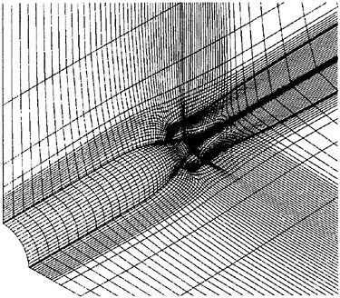
Figure 1
Example Grid
The specific areas of grid generation which have been addressed are:
-
Improved topology creation, with C-C grid around all appendages
-
Detailed changes to surface grid generation to enable a wider range of configurations
-
Improved accuracy and stability in the refinement algorithms for viscous grid generation to enable high quality grids with appropriate near wall grid spacings
The SAUNA grid generation methodology allows direct comparisons to be made between down-to-the-wall and wall function approaches. For simple bodies, the grid refinement algorithm acts along a series of splines defined by a background O-O topology grid. To obtain suitable grid support for a particular turbulence model, the only changes which need to be made are the first cell spacing and the number of cells in the innermost blocks. This ensures that the grid resolution for the pressure field is maintained, irrespective of the required turbulence model and Reynolds’ number.
Flow solution algorithm
The flow solver used for this work was CFX4.2 produced by CFDS International. CFX4.2 is a commercially available multi-block structured, control volume based finite volume flow code. A third order accurate scheme for the convection terms was used and a PISO algorithm for pressure correction. The convection scheme ensures the turbulence parameters are positive throughout the calculations. The grids produced by SAUNA were converted into a smaller number of blocks to assist efficient vectorisation for the Cray C90.
To ensure accuracy and robustness for such high Reynolds’ number problems, with small grid spacing, it was necessary to maintain high numerical precision at every stage in the flow solution process.
Results for the Suboff AFF1 configuration
Preliminary computations for the AFF1 configuration were made using CFX4.2. These computations were used to investigate the performance of the three turbulence models over a range of grid resolutions and Reynolds’ numbers. All computational residuals were reduced by at least four orders of magnitude. The results were found to be consistent for the higher grid resolutions. All the results shown in this section are for the highest grid resolution.
The number of cells in the three background axisymmetric grids was 5,000, 10,000 and 25,000. The number of cells in the direction normal to the wall in the innermost layers was 41 for the Wilcox and Menter models and 25 for the RNG model with appropriate first cells spacing for each Reynolds number. Flow predictions were carried out for Reynolds’ number of 1.2×10⁷, 3×10⁷, 6×10⁷, 1.2×10⁸, 3×10⁸, 6×10⁸ and 1.2×10⁹ for each of the turbulence models.
Comparison of the boundary layer profiles of the axial velocity component and the turbulent kinetic energy respectively are given in figure 2 and 3 for the axial stations x/L=0.978 and 1.040. Profiles for the measured data are compared with the computed results for the model scale Reynolds’ number of 1.2×10⁷.
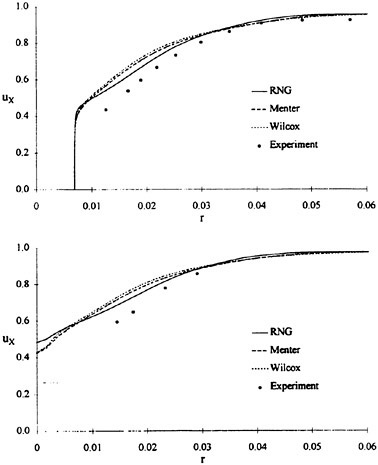
Figure 2
Axial velocity component at x=0.978 and x=1.040
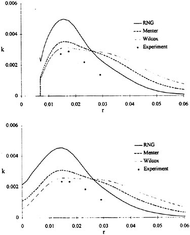
Figure 3
Turbulent kinetic energy at x=0.978 and x=1.040
Figure 4 shows the pressure and skin friction coefficients along the length of the hull for each of the turbulence models for Reynolds numbers 1.2×10⁷, 1.2×10⁸ and 1.2×10⁹.
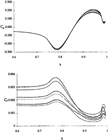
Figure 4
Pressure and skin friction coefficients along the hull for each Reynolds’ number
Comparisons of the profiles for the axial velocity component and turbulent kinetic energy for the boundary layer at x=0.978 and for the wake along the axis are given in figures 5 to 7. Comparison between each of the turbulence models for three Reynolds’ numbers of 1.2×10⁷, 1.2×10⁸ and 1.2×10⁹ are shown in figures 5, 6 and 7 for the boundary layer and wake profiles. The data for the RNG, Menter and Wilcox turbulence models are given as solid, dashed and dotted lines respectively.
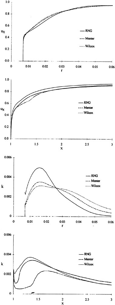
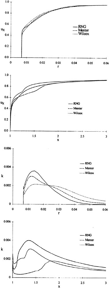
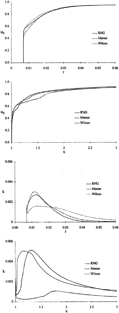
Figure 7
Boundary layer and wake profiles at Re=1.2×10⁹
The volumetric wake fraction w2 is given by
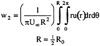
This volumetric wake fraction at x=0.978 and x=1.040 for the complete range Reynolds’ numbers and turbulence models is given in table 4.
Table 4
Volumetric wake fractions
|
|
x=0.978 |
x=1.040 |
||||
|
Re |
RNG |
Menter |
Wilcox |
RNG |
Menter |
Wilcox |
|
1.2×10⁷ |
0.686 |
0.708 |
0.720 |
0.759 |
0.775 |
0.786 |
|
3.0×10⁷ |
0.716 |
0.728 |
0.747 |
0.785 |
0.790 |
0.810 |
|
6.0×10⁷ |
0.734 |
0.742 |
0.766 |
0.800 |
0.803 |
0.827 |
|
1.2×10⁸ |
0.754 |
0.756 |
0.777 |
0.818 |
0.815 |
0.836 |
|
3.0×10⁸ |
0.776 |
0.760 |
0.795 |
0.838 |
0.819 |
0.852 |
|
6.0×10⁸ |
0.789 |
0.774 |
0.808 |
0.848 |
0.832 |
0.863 |
|
1.2×10⁹ |
0.804 |
0.790 |
0.816 |
0.862 |
0.845 |
0.870 |
Results for the Suboff AFF4 configuration
A series of calculations were performed for the AFF4 configuration using a number of grid resolutions for the underlying pressure field suitable for ‘wall functions’ and for ‘down-to-the-wall’ predictions. The topology of the local grids around the components was chosen to produce an O-O grid around the hull with C-C grids around the aft appendages. This provides the most efficient grid structure while maintaining sufficient grid support in the wake of the appendages. The number of cells necessary to obtain the required y+ spacings and maintain a reasonable expansion ratio in the innermost, viscous grid layers for the ‘down-to-the-wall’ grids meant that approximately 50% of the cells were dedicated to the resolution of the viscous boundary layer and wakes.
Therefore, for underlying grid resolutions of 200,000 and 400,000 cells for the pressure field, approximately 250,000 and 500,000 cells were used for the ‘wall function’ grid with 500,000 and 1,000,000 cells used for the equivalent ‘down-to-the-wall’ grids. The same number of cells and first cell spacing in the innermost layers as described for the AFF1 configuration was used for each turbulence model and Reynolds’ number.
Initial flow computations with the three turbulence models indicated that the convergence of the flow solution algorithm was incorrect in the wake for the two ‘down-to-the-wall’ models. There were only very weak wakes behind the appendages, especially for the Wilcox model. There was also evidence that the multi-block scheme was not producing a symmetric solution to the problem, especially for the turbulence fields.
To obtain reasonable solutions for the ‘down-to-the-wall’ models, it was necessary to increase the first cell spacing in the wakes downstream of the appendages. It was also necessary to under-relax the solution procedure in CFX4.2 to obtain symmetric solutions. A larger number of iterations were required to develop the wake profiles downstream of the appendages. On examination of the results for the 500,000 cell cases, it was clear that the wake field for the Wilcox model was not sufficiently developed although the solution residuals had ‘converged’ by at least four orders of magnitude. Therefore, only results for the RNG and Menter turbulence models for Reynolds’ number of 1.2×10⁷, 1.2×10⁸ and 1.2×10⁹ for the fine grids are given in this paper.
Examination of the results from the RNG turbulence model showed consistent trends in the development of the flow around the AFF4 configuration. There was evidence of the development of small vortex structures embedded in the boundary layer of the hull which showed little variation with Reynolds’ number. The thickness of the wake structure behind the appendage reduced, and the relative intensity of the turbulent kinetic energy in the embedded vortices increased as the Reynolds’ number increased. However, the results for the Menter turbulence model showed different trends. The size and strength of the embedded vortices increased as the Reynolds’ number increased and the position of the stagnation point forward of the appendages moved upstream. Overall, the Menter turbulence model showed considerably more activity than the RNG model, especially in the boundary layer, which increased as the Reynolds’ number increased. This is illustrated by plots of the measured and computed flow parameters for radii at r/R=0.25, 0.3, 0.4 and 0.5 in the plane of the propulsor.
Figure 8 shows the measured flow parameters ux, ur and k for each of the radii. The data are plotted at two degree intervals. Comparison between the Menter and RNG turbulence models for each Reynolds’ number is given in figures 9 to 14. These figures show the variation of the computed flow parameters ux, ur, k and ν for the same radii and axial position as the measured data. The data are plotted at intersections with the grid.
Contours of the axial velocity magnitude in the plane of the propulsor at x=0.978 for each of the Reynolds’ numbers are given in figures 15 and 16 for the Menter and RNG models respectively. The contours range from 0.1 to 1.0 with an increment of 0.05.
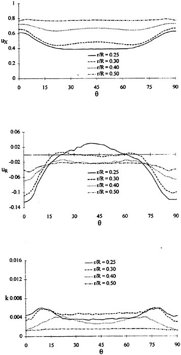
Figure 8
Measured experimental data at Re=1.2×10⁷
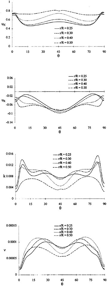
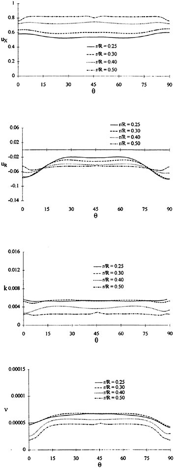
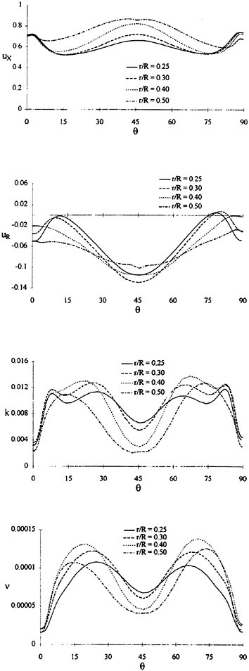
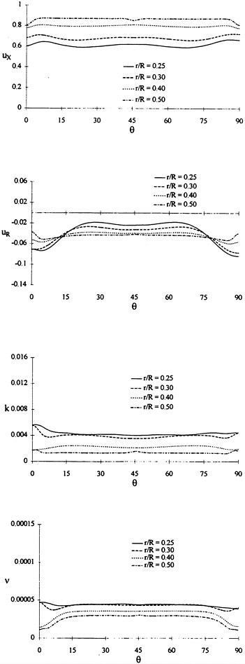
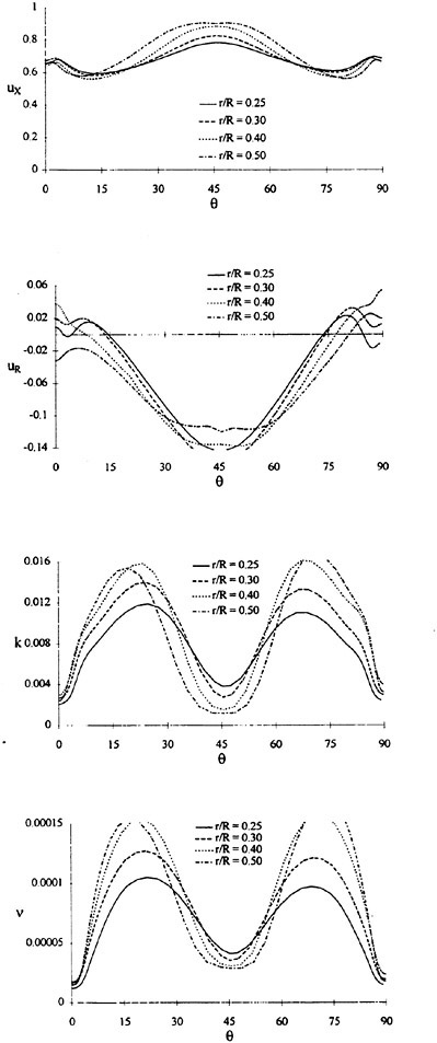
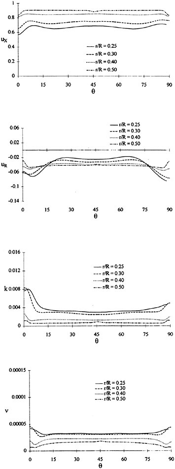
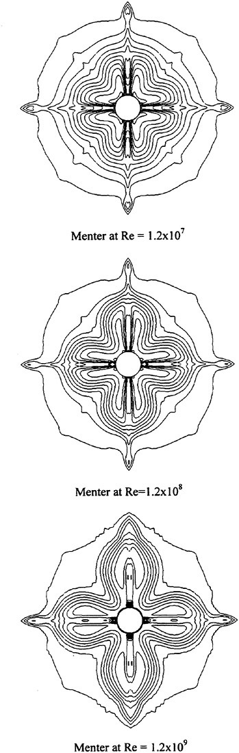
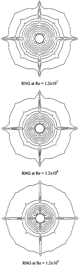
Discussion
There are differences between the turbulence models which become more pronounced as the Reynolds’ number increases. The overall shape and features of the profiles and contours at the model scale Reynolds’ number are fairly similar but the results at full scale are quite different. It is not yet certain that these differences are purely due to the turbulence model and the associated boundary conditions.
Further examination of the profiles for the AFF1 configuration show that the boundary layer profile is sensitive to the initial and boundary conditions. In particular, the estimates of boundary layer thickness, skin friction coefficient and the overshoot velocity all contribute to systematic differences in the predictions at model scale. In addition, although the value of the background turbulence is set at the start of the iterative scheme, the final value reduced by up to an order of magnitude. However, for this exercise, it was necessary to maintain a consistent specification of the initial condition which encompassed a range of Reynolds’ numbers.
Examination of the wake profiles for AFF4 shows that the Menter turbulence model is predicting larger variations in the velocity and turbulence parameters than the RNG model at model scale. When the axial velocity component in figures 9 and 10, is compared with the measured data in figure 8, the overall characteristics of the wake are better captured by the Menter model. This would indicate that the Menter model predicts the magnitude of the wake harmonics better that the standard RNG model. However, when comparison is made between the radial velocity component, the Menter model predicts a deep minimum at θ=45°. This feature is absent in the experiment data and in the RNG predictions. The turbulent kinetic energy predicted by the Menter model is twice the experimental data on the innermost rake, rising to six times on the outermost rake. However, the values predicted on the plane of symmetry are close to the experimental values and on the inner rakes, the general behaviour of the experiment is followed closely. The peaks are more compact and there is a reduction from a relatively uniform value at θ=45°. The RNG predictions are featureless by comparison. The general levels of the experiment are predicted, but the features are either missing or very weak. This is particularly true in the wakes of the appendages.
As Reynolds number increases, the flow features of the Menter predictions intensify. This is most apparent in the central region, away from the plane of symmetry and just outside of the appendage wakes. The radial velocity has its maximum on the bisecting plane and there are peaks of turbulent kinetic energy and of eddy viscosity on either side of this plane. The peaks start developing soon after the hull radius starts to decrease and appear to be associated with the outer part of the hull shear layer where blending between the ω and ε models occurs. The only no-slip surface in this region is the hull with smoothly varying normals. The operation of the blending function is therefore unlikely to be complicated by secondary flows in this region. This points to a potential mismatch between the conditions inside and outside of the hull shear layer rather than a natural phenonema. This is supported by the change observed in the ratio of μT/μ in the outer flow domain and the comparison with experimental data at model scale.
In contrast, the RNG predictions change relatively little and there is no intensification of flow features. There is a gradual rise in axial velocity and a gradual reduction in both the turbulent kinetic energy and the eddy viscosity. The variation in radial velocity increases slightly. Overall, the predictions also become less symmetrical as the Reynolds number increases.
There appears to be some dependency in the predicted flow field for both turbulence models on the order in which the flow solver addresses the blocks of the grid. This dependency becomes more pronounced as Reynolds’ number increases. The severity can be gauged from the extent of the deviation from symmetry in the radial profiles. The major concern that this raises is the level of convergence of the predictions. For the RNG predictions, this is unlikely to be an issue; the residuals have fallen by at least four orders of magnitude and the maximum change in the velocity variables, at least, is well below 0.1% of free stream. For the Menter predictions, although a larger number of iterations were used for each flow prediction, a greater degree of under-relaxation was required to maintain symmetric solutions. Therefore, the reduction in residuals was generally smaller than for the corresponding RNG prediction and the maximum change in velocity somewhat larger.
Conclusions
Predictions of the flow around an appended geometry have been obtained for a range of Reynolds’ numbers for different turbulence models. To obtain meaningful comparisons between the turbulence models for the range of Reynolds’ number it was necessary to increase the resolution and accuracy of all stages of the CFD process. The reliability of such comparison depends on how well the flow features are resolved. This imposes an increased level of rigour and control of factors such as grid resolution, computational accuracy and numerical precision. This also extends to the critical assessment of the predicted flow field, and its level of convergence.
The RNG turbulence model in conjunction with wall functions and the Menter turbulence model can make predictions from model to full scale for appended and unappended bodies. For the AFF1 configuration, there is some consistency in the scaling of their predictions. This is not yet the case for the more complex AFF4 configuration. As a whole, the predictions point to an increased sensitivity of the Menter model to changes in Reynolds number. However, insufficient numerical implementations have been used to come to definitive conclusion on this matter.
The performance of the particular solution algorithm appears to reduce somewhat when applied to appended geometries, especially when using the ‘down-to-the-wall’ turbulence models. There are some difficulties with the reliability of the solution algorithm, associated with the multi-block nature of the method.
Further work is required to clarify the requirements for grid resolution and numerical stability for the more complex ‘down-to-the wall’ turbulence models, especially for fully appended geometries.
1. Bull P., “The Validation of CFD Prediction of Nominal Wake for the SUBOFF Fully Appended Geometry”, Proceedings of 21st Symposium of Naval Hydrodynamics, Trondheim, Norway 1996.
2. Eça L and Hoekstra M., “Numerical Calculations of Ship Stern Flows at Full Scale Reynolds’ Numbers”, Proceedings of 21st Symposium of Naval Hydrodynamics, Trondheim, Norway 1996.
3. Ju S., “Numerical Study of Ship Stern and Wake Flows at Model Scale and Full-Scale Reynolds; Numbers”, IIHR Report no 323, 1991
4. Watson S.J.P. and Bull P.W., “The Scaling of High Reynolds’ Number Viscous Flow Predictions using CFD Techniques”, Third Osaka Colloquium on Advanced CFD Applications to Ship Flow and Hull Form Design, Osaka, Japan, 1998.
5. Sotiropoulos F. and Patel V.C., “Second moment modelling for ship-stern and wake flows”, Proceedings of CFD Workshop for Improvement of Hull Form Designs, Toyko, 1994.
6. Deng G., Visonneau M., “Evaluation of Eddy Viscosity and Second-Moment Turbulence Closures for Steady Flows Around Ships”. Proceedings of 21st Symposium on Naval Hydrodynamics, Trondheim, Norway, June 1996.
7. Larsson L., Patel V.C. and Dyne G., (ed), Proceedings of 1990 SSPA-CTH-IIHR Workshop on Ship Viscous Flow, 1990.
8. Wilcox D.C, “Turbulence Modelling for CFD” 1994, DCW Industries.
9. Menter F.R., “Influence of freestream values on k-ω turbulence model prediction”, AIAA Journal 30.6, 1992.
10 “CFX4.2 User Guide”, 1997, CFX International, Harwell Laboratory, Oxfordshire, OX11 0RA, United Kingdom
11 “SAUNA Release 3.0 Volume 1 User Guide”, 1998, ARA Limited, Manton Lane, Bedford MK41 7PF, United Kingdom.


