
2
Rise of Earthquake Science
Earthquakes have engaged human inquiry since ancient times, but the scientific study of earthquakes is a fairly recent endeavor. Instrumental recordings of earthquakes were not made until the last quarter of the nineteenth century, and the primary mechanism for the generation of earthquake waves—the release of accumulated strain by sudden slippage on a fault—was not widely recognized until the beginning of the twentieth century. The rise of earthquake science during the last hundred years illustrates how the field has progressed through a deep interplay among the disciplines of geology, physics, and engineering (1). This chapter presents a historical narrative of the development of the basic concepts of earthquake science that sets the stage for later parts of the report, and it concludes with some historical lessons applicable to future research.
2.1 EARLY SPECULATIONS
Ancient societies often developed religious and animistic explanations of earthquakes. Hellenic mythology attributed the phenomenon to Poseidon, the god of the sea, perhaps because of the association of seismic shaking with tsunamis, which are common in the northeastern Mediterranean (Figure 2.1). Elsewhere, earthquakes were connected with the movements of animals: a spider or catfish (Japan), a mole or elephant (India), an ox (Turkey), a hog (Mongolia), and a tortoise (Native America). The Norse attributed earthquakes to subterranean writhing of the imprisoned god Loki in his vain attempt to avoid venom dripping from a serpent’s tooth.
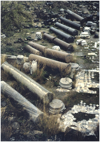
FIGURE 2.1 The fallen columns in Susita (Hypos) east of the Sea of Galilee from a magnitude ~7.5 earthquake on the Dead Sea transform fault in A.D. 749. SOURCE: A. Nur, And the walls came tumbling down, New Scientist, 6, 45-48, 1991. Copyright A. Nur.
Some sought secular explanations for earthquakes and their apocalyptic consequences (Box 2.1, Figure 2.2). For example, in 31 B.C. a strong earthquake devastated Judea, and the historian Josephus recorded a speech by King Herod given to raise the morale of his army in its aftermath (2): “Do not disturb yourselves at the quaking of inanimate creatures, nor do you imagine that this earthquake is a sign of another calam-
|
BOX 2.1 Ruins of the Ancient World The collision of the African and Eurasian plates causes powerful earthquakes in the Mediterranean and Middle East. Some historical accounts document the damage from particular events. For example, a Crusader castle overlooking the Jordan River in present-day Syria was sheared by a fault that ruptured it at dawn on May 20, 1202.1 In most cases, however, such detailed records have been lost, so that the history of seismic destruction can be inferred only from archaeological evidence. Among the most convincing is the presence of crushed skeletons, which are not easily attributable to other natural disasters or war and have been found in the ruins of many Bronze Age cities, including Knossos, Troy, Mycenae, Thebes, Midea, Jericho, and Megiddo. Recurring earthquakes may explain the repeated destruction of Troy, Jericho, and Megiddo, all built near major active faults. Excavation of the ancient city of Megiddo—Armageddon in the Biblical prophecy of the Apocalypse—reveals at least four episodes of massive destruction, as indicated by widespread debris, broken pottery, and crushed skeletons.2 Similarly, a series of devastating earthquakes could have destabilized highly centralized Bronze Age societies by damaging their centers of power and leaving them vulnerable to revolts and invasions.3 Historical accounts document such “conflicts of opportunity” in the aftermath of earthquakes in Jericho (~1300 B.C.), Sparta (464 B.C.), and Jerusalem (31 B.C.). |
ity; for such affections of the elements are according to the course of nature, nor does it import anything further to men than what mischief it does immediately of itself.”
Several centuries before Herod’s speech, Greek philosophers had developed a variety of theories about natural origins of seismic tremors based on the motion of subterranean seas (Thales), the falling of huge blocks of rock in deep caverns (Anaximenes), and the action of internal fires (Anaxagoras). Aristotle in his Meteorologica (about 340 B.C.) linked earthquakes with atmospheric events, proposing that wind in underground caverns produced fires, much as thunderstorms produced lightning. The bursting of these fires through the surrounding rock, as well as the collapse of the caverns burned by the fires, generated the earthquakes. In support of this hypothesis, Aristotle cited his observation that earthquakes tended to occur in areas with caves. He also classified earthquakes according to whether the ground motions were primarily vertical or hori-

FIGURE 2.2 The remains of a family—a man, woman, and child (small skull visible next to the woman’s skull)—crushed to death in A.D. 365 in the city of Kourian on the island of Cyprus when their dwelling collapsed on top of them during an earthquake. SOURCE: D. Soren, The day the world ended at Kourion, National Geographic, 30-53, July 1988; Copyright Martha Cooper.
zontal and whether they released vapor from the ground. He noted that “places whose subsoil is poor are shaken more because of the large amount of the wind they absorb.” The correlation he observed between the intensity of the ground motions and the weakness of the rocks on which structures are built remains central to seismic hazard analysis.
2.2 DISCOVERY OF SEISMIC FAULTING
Aristotle’s ideas and their variants persisted well into the nineteenth century (3). In the early 1800s, geology was a new scientific discipline, and most of its practitioners believed that volcanism caused earthquakes, both of which are common in geologically active regions. A vigorous adherent to the volcanic theory was the Irish engineer Robert Mallet, who coined the term seismology in his quantitative study of the 1857 earthquake in southern Italy (4). By this time, however, evidence had been accumulating that earthquakes are incremental episodes in the building of mountain belts and other large crustal structures, a process that geologists named tectonics. Charles Lyell, in the fifth edition of his seminal book The Principles of Geology (1837), was among the first to recognize that large earthquakes sometimes accompany abrupt changes in the ground surface (5). He based this conclusion on reports of the 1819 Rann of Cutch (Kachchh) earthquake in western India—near the disastrous January 26, 2001, Bhuj earthquake— and, in later editions, on the Wairarapa, New Zealand, earthquake of 1855. A protégé of Lyell’s, Charles Darwin, experienced a great earthquake while visiting Chile in 1835 during his voyages on the H.M.S. Beagle. Following the earthquake, he and Captain FitzRoy noticed that in many places the coastline had risen several meters, causing barnacles to die because of prolonged exposure to air. He also noticed marine fossils in sediments hundreds of meters above the sea and concluded that seismic uplift was the mechanism by which the mountains of the coast had risen. Darwin applied James Hutton’s principle of uniformitarianism—“the present is the key to the past”—and inferred that the mountain range had been uplifted incrementally by many earthquakes over many millennia (6).
Fault Slippage as the Geological Cause of Earthquakes
The leap from these observations to the conclusion that earthquakes result from slippage on geological faults was not a small one. The vast majority of earthquakes are accompanied by no surface faulting, and even when such ruptures had been found, questions arose as to whether the ground breaking shook the Earth or the Earth shaking broke the ground. Moreover, the methodology for mapping fault displacements and understanding their relationships to geological deformations, the discipline of structural geology, had not yet been systematized. A series of field studies—by G.K. Gilbert in California (1872), A. McKay in New Zealand (1888), B. Koto in Japan (1891), and C.L. Griesbach in Baluchistan (1892)—demonstrated that fault motion generates earthquakes, thereby documenting that the surface faulting associated with each of these earthquakes was consistent with the long-term, regional tectonic deformation that geologists had mapped (Figure 2.3).
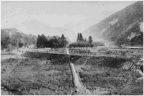
FIGURE 2.3 Photograph of the 1891 Nobi (Mino-Owari) earthquake scarp at Midori, taken by B. Koto, a professor of geology at the Imperial University of Tokyo. Based on his geological investigations, Koto concluded, “The sudden elevations, depressions, or lateral shiftings of large tracts of country that take place at the time of destructive earthquakes are usually considered as the effects rather than the cause of subterranean commotion; but in my opinion it can be confidently asserted that the sudden formation of the ‘great fault of Neo’ was the actual cause of the great earthquake.” This photograph appeared in The Great Earthquake in Japan, 1891, published by the Seismological Society of Japan, which was one of the first comprehensive scientific reports of an earthquake. The damage caused by the Nobi earthquake motivated Japan to create an Earthquake Investigation Committee, which set up the first government-sponsored research program on the causes and effects of earthquakes. SOURCE: J. Milne and W.K. Burton, The Great Earthquake in Japan, 1891, 2nd ed., Lane, Crawford & Co., Yokohama, Japan, 69 pp. + 30 plates, 1892.
Among the geological investigations of this early phase of tectonics, Gilbert’s studies in the western United States were seminal for earthquake science. From the new fault scarps of the 1872 Owens Valley earthquake, he observed that the Sierra Nevada, bounding the west side of the valley, had moved upward and away from the valley floor. This type of faulting was consistent with his theory that the Basin and Range Province between the Sierra Nevada and the Wasatch Mountains of Utah had been formed by tectonic extension (7). He also recognized the similarity of the
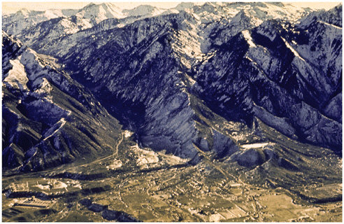
FIGURE 2.4 Aerial view, Salt Lake City, showing the scarps of active normal faults of the Wasatch Front, first recognized by G.K. Gilbert. SOURCE: Utah Geological Survey.
Owens Valley break to a series of similar piedmont scarps along the Wasatch Front near Salt Lake City (Figure 2.4). By careful geological analysis, he documented that the Wasatch scarps were probably caused by individual fault movements during the recent geological past. This work laid the foundation for paleoseismology, the subdiscipline of geology that employs features of the geological record to deduce the fault displacement and age of individual, prehistoric earthquakes (8).
Geological studies were supplemented by the new techniques of geodesy, which provide precise data on crustal deformations. Geodesy grew out of two practical arts, astronomical positioning and land surveying, and became established as a field of scientific study in the mid-nineteenth century. One of the first earthquakes to be measured geodetically was the Tapanuli earthquake of May 17, 1892, in Sumatra, which happened during a triangulation survey by the Dutch Geodetic Survey. The surveyor in charge, J.J.A. Müller, discovered that the angles between the survey monuments had changed during the earthquake, and he concluded that a horizontal displacement of at least 2 meters had occurred along a structure later recognized to be a branch of the Great Sumatran fault. R.D. Oldham
of the Geological Survey of India inferred that the changes in survey angles and elevations following the great Assam earthquake of June 12, 1897, were due to co-seismic tectonic movements. C.S. Middlemiss reached the same conclusion for the Kangra earthquake of April 4, 1905, also in the well-surveyed foothills of the Himalaya (9).
Mechanical Theories of Faulting
The notion that earthquakes result from fault movements linked the geophysical disciplines of seismology and geodesy directly to structural geology and tectonics, whose practitioners sought to explain the form, arrangement, and interrelationships among the rock structures in the upper part of the Earth’s crust. Although Hutton, Lyell, and the other founders of the discipline of geology had investigated the great vertical deformations required by the rise of mountain belts, the association of these deformations with large horizontal movements was not established until the latter part of the nineteenth century (10). Geological mapping showed that some horizontal movements could be accommodated by the ductile folding of sedimentary strata and plastic distortion of igneous rocks, but that much of the deformation takes place as cataclastic flow (i.e., as slippage in thin zones of failure in the brittle materials that make up the outer layers of the crust). Planes of failure on the larger geological scales are referred to as faults, classified as normal, reverse, or strike-slip according to their orientation and the direction of slip (Figure 2.5).
In 1905, E.M. Anderson (11) developed a successful theory of these faulting types, based on the premises that one of the principal compressive stresses is oriented vertically and that failure is initiated according to a rule published in 1781 by the French engineer and mathematician Charles Augustin de Coulomb. The Coulomb criterion states that slippage occurs when the shear stress on a plane reaches a critical value tc that depends linearly on the effective normal stress sneff acting across that plane:
tc = t0 + µsneff, (2.1)
where t0 is the (zero-pressure) cohesive strength of the rock and µ is a dimensionless number called the coefficient of internal friction, which usually lies between 0.5 and 1.0. Anderson’s theory made quantitative predictions about the angles of shallow faulting that fit the observations rather well (except in regions where fault planes were controlled by strength anisotropy like sedimentary layering). However, it could not explain the existence of large, nearly horizontal thrust sheets that formed at deeper structural levels in many mountain belts. Owing to the large lithostatic load, the total normal stress sn acting on such fault planes was
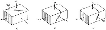
FIGURE 2.5 Fault types showing principal stress axes and Coulomb angles. For a typical coefficient of friction in rocks (µ ˜ 0.6), the Coulomb criterion (Equation 2.1) implies that a homogeneous, isotropic material should fail under triaxial stress (s1 > s2 > s3) along a plane that contains the s2 axis and lies at an angle about 30° to the s1 direction. According to Anderson’s theory, normal faults should therefore occur where the vertical stress sV is the maximum principal stress s1, and the initial dips of these extensional faults should be steep (about 60°); reverse faults (sV = s3) should initiate as thrusts with shallow dips of about 30°, and strike-slip faults (sV = s2) should develop as vertical planes striking at about 30° to the s1 direction. SOURCE: Reprinted from K. Mogi, Earthquake Prediction, Academic Press, Tokyo, 355 pp., 1985, Copyright 1985 with permission from Elsevier Science.
much greater than any plausible tectonic shear stress, so it was difficult to see how failure could happen. M.K. Hubbert and W.W. Rubey resolved this quandary in 1959 (12) by recognizing that the effective normal stress in the Coulomb criterion should be the difference between sn and the fluid pressure Pf:
sneff = sn – Pf. (2.2)
They proposed that overthrust zones were overpressurized; that is Pf in these zones was substantially greater than the pressure expected for hydrostatic equilibrium and could approach lithostatic values (13). Hence, sneff could be much smaller than sn. Overpressurization may explain why some faults, such as California’s San Andreas, appear to be exceptionally weak.
Elastic Rebound Model
When a 470-kilometer segment of the newly recognized San Andreas rift ruptured across northern California in 1906 (Box 2.2, Figures 2.6 and 2.7), both geologists and engineers jumped at the opportunity to observe first-hand the effects of a major earthquake. Three days after the earthquake, while the fires of San Francisco were still smoldering, California Governor George C. Pardee appointed a State Earthquake Investigation
|
BOX 2.2 San Francisco, California, 1906 At approximately 5:12 a.m. local time on April 18, 1906, a small fracture nucleated on the San Andreas fault at a depth of about 10 kilometers beneath the Golden Gate (20). The rupture expanded outward, quickly reaching its terminal velocity of about 2.5 kilometers per second (5600 miles per hour). Its upper front broke through the ground surface at the epicenter within a few seconds, and its lower front decelerated as it spread downward into the more ductile levels of the middle crust, while the two sides continued to propagate in opposite directions along the San Andreas. Near the epicenter, the rupture displaced the opposite sides of the fault rightward by an average of about 4 meters (a right-lateral strike-slip). On the southeastern branch, the total slip diminished as the rupture traveled down the San Francisco peninsula and vanished 100 kilometers away from the epicenter. To the northwest, the fracture ripped across the neck of the Point Reyes peninsula and entered Tomales Bay, where the total slip increased to 7 meters, sending out seismic waves that damaged Santa Rosa, Fort Ross, and other towns of the northern Coast Ranges. The rupture continued up the coast to Point Arena, where it went offshore, eventually stopping near a major bend in the fault at Cape Mendocino (Figure 2.6). At least 700 people were killed, perhaps as many as 3000, and many buildings were severely damaged.1 In San Francisco, the quake ignited at least 60 separate fires, which burned unabated for three days, consuming 42,000 buildings and destroying a considerable fraction of the West Coast’s largest city. |
Commission, headed by Berkeley Professor Andrew C. Lawson, to coordinate a wide-ranging set of scientific and engineering studies (14). The first volume of the Lawson Report (1908) compiled reports by more than 20 specialists on a variety of observations: the geological setting of the San Andreas; the fault displacements inferred from field observations and geodetic measurements; reports of the arrival time, duration, and intensity of the seismic waves; seismographic recordings from around the world; and detailed surveys of the damage to structures throughout Northern California. The latter demonstrated that the destruction was closely related to building design and construction, as well as to local geology. The intensity maps of San Francisco clearly show that some of the strongest shaking occurred in the soft sediment of China Basin and in the present Marina district, two San Francisco neighborhoods that would be severely damaged in the Loma Prieta earthquake some 83 years later (15). This interdiscipli-
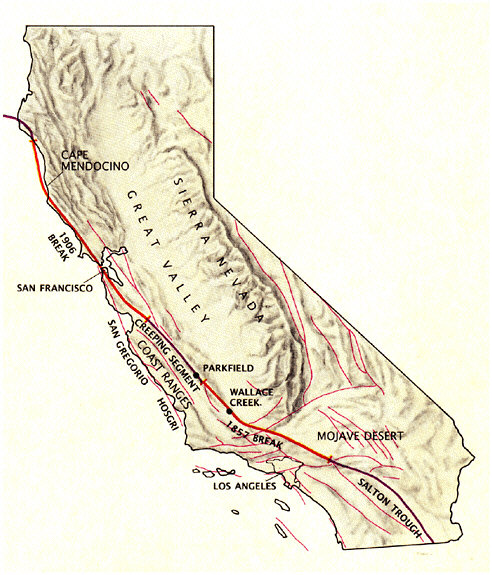

FIGURE 2.7 Panoramic view of the ruins of San Francisco after the April 1906 earthquake and fire, viewed from the Stanford Mansion site. SOURCE: Lester Guensey, Library of Congress, Prints and Photographs Division, [Lc-USZ62-123408 DLC].
nary synthesis is still being mined for information about the 1906 earthquake and its implications for future seismic activity (16).
Professor Henry Fielding Reid of Johns Hopkins University wrote the second volume of the Lawson Report (1910), presenting his celebrated elastic rebound hypothesis. Reid’s 1911 follow-up paper (17) summarized his theory in five propositions:
-
The fracture of the rocks, which causes a tectonic earthquake, is the result of elastic strains, greater than the strength of the rock can withstand, produced by the relative displacements of neighboring portions of the earth’s crust.
-
These relative displacements are not produced suddenly at the time of the fracture, but attain their maximum amounts gradually during a more or less long period of time.
-
The only mass movements that occur at the time of the earthquake are the sudden elastic rebounds of the sides of the fracture towards positions of no elastic strain; and these movements extend to distances of only a few miles from the fracture.
-
The earthquake vibrations originate in the surface of the fracture; the surface from which they start is at first a very small area, which may quickly become very large, but at a rate not greater than the velocity of compressional elastic waves in rock.
-
The energy liberated at the time of an earthquake was, immediately before the rupture, in the form of energy of elastic strain of the rock.
Today all of these propositions are accepted with only minor modifications (18). Although some geologists, for at least the latter half of the nineteenth century, had considered the notion that most large earthquakes result from fault slippage, Reid’s hypothesis was boldly revolutionary. The horizontal tectonic displacements he postulated had no well-estab-

lished geologic basis, for example, and they would remain mysterious until the plate-tectonic revolution of the 1960s (19).
2.3 SEISMOMETRY AND THE QUANTIFICATION OF EARTHQUAKES
In 1883, the English mining engineer John Milne suggested that “it is not unlikely that every large earthquake might with proper appliances be recorded at any point of the globe.” His vision was fulfilled six years later when Ernst von Rebeur-Paschwitz recorded seismic waves on delicate horizontal pendulums at Potsdam and Wilhemshaven in Germany from the April 17, 1889, earthquake in Tokyo, Japan. By the turn of the century, the British Association for the Advancement of Science was sponsoring a global network of more than 40 stations, most equipped with instruments of Milne’s design (21); other deployments followed, expanding the coverage and density of seismographic recordings (22). Working with records of the great Assam earthquake of June 12, 1897, Oldham identified three basic wave types: the small primary (P or compressional) and secondary (S or shear) waves that traveled through the body of the Earth and the “large” (L) waves that propagated across its outer surface (23).
Hypocentral Locations and Earth Structure
Milne investigated the velocities of the P, S, and L waves by plotting their travel times as a function of distance for earthquakes whose location had been fixed by local observations. From curves fit to these travel times, he could then determine the distance from the observing stations to an event with an unknown epicenter, and he could fix its location from the
intersection of arcs drawn at the estimated distance from three or more such stations. By applying this simple technique, he and others began to compile catalogs of instrumentally determined earthquake epicenters (24).
Improved locations meant that seismologists could use the travel time of the seismic waves to develop better models of the variations of wave velocities with depth, which in turn could be used to improve the location of the earthquake’s initial radiation (hypocenter), as well as its origin time. This cycle of iterative refinement of Earth models and earthquake locations, along with advances in the distribution and quality of the seismometer networks, steadily decreased the uncertainties in both. It also led to some major discoveries. In 1906, Oldham presented the first seismological evidence that the Earth had a central core, and in 1914, Beno Gutenberg obtained a relatively precise depth (about 2900 kilometers) to the boundary between the core and the solid-rock shell or mantle (German for coat) surrounding it. From regional recordings of the 1909 Croatian earthquake, the Serbian seismologist Andriji Mohorovicic discovered the sharp increase in seismic velocities that bears his name, often abbreviated the Moho, which separates the lighter, more silica-rich crust from the ultramafic (iron- and magnesium-rich) mantle.
After Milne’s death in 1913, H.H. Turner, an Oxford professor, took over the determination of earthquake hypocenters and origin times. Turner’s efforts to compile earthquake data systematically led, after the First World War, to the founding of the International Seismological Summary (ISS) (25). While preparing the ISS bulletins, Turner (1922) noticed some events with anomalous travel times, which he proposed had hypocenters much deeper than that of typical earthquakes. In 1928, Kiyoo Wadati established the reality of such “deep-focus” earthquakes as much as 700 kilometers beneath volcanic arcs such as Japan and the Marianas, and he subsequently delineated planar regions of seismicity (now called Wadati-Benioff zones) extending from the ocean trenches at the face of the arcs down to these deep events. The Danish seismologist Inge Lehmann discovered the Earth’s inner core in 1936; this “planet within a planet” has since been shown to be a solid metallic sphere two-thirds the size of the Moon at the center of the liquid iron-nickel outer core. By the time Harold Jeffreys and Keith Bullen finalized their travel-time tables in 1940, the Earth’s internal structure was known well enough to estimate the hypocenter of large earthquakes with a standard error often less than 10 kilometers and origin time with a standard error of less than 2 seconds (26).
Earthquake Magnitude and Energy
The next important step in the development of instrumental seismology was the quantification of earthquake size. Maps of seismic damage
were made in Italy as early as the late eighteenth century. In the 1880s, M.S. Rossi of Italy and F. Forel of Switzerland defined standards for grading qualitative observations by integer values that increase with the amount of shaking and disruption. Versions of their “intensity scale,” as modified by G. Mercalli and others, are still used to map intensity after strong events (27), but they do not measure the intrinsic size of an earthquake, nor can they be applied to events that humans have not felt and observed (i.e., almost all earthquakes). The availability of instrumental recordings and the desire to standardize the seismological bulletins motivated seismologists to estimate the intrinsic size of earthquakes by measuring the amplitude of the seismic waves at a station and correcting them for propagation effects, such as the spreading out of wave energy and its attenuation by internal friction. Several such scales were developed, including one by Wadati in 1931, but the most popular and successful schemes were based on the standard magnitude scale that Charles Richter of Caltech published in 1935.
Richter recognized that seismographic amplitude provides a first-order measure of the radiated energy but that these data are highly variable depending on the type of seismograph, distance to the earthquake, and local site conditions. To normalize for these factors, he considered only southern California earthquakes recorded on Caltech’s standardized network of Wood-Anderson torsion seismometers (28). He defined the local magnitude scale for such events by the formula
ML = log A – log A0, (2.3)
where A is the maximum amplitude of the seismic trace on the standard seismogram; A0 is the amplitude at that same distance for a reference earthquake with ML = 0; and all logarithms are base 10. He fixed the reference level A0 by specifying a magnitude-zero earthquake as an event with an amplitude of 1 micron on a standard Wood-Anderson seismogram at a distance of 100 kilometers (29). An earthquake of magnitude 3.0 thus had an amplitude of 1 millimeter at 100 kilometers, which was about the smallest level measurable on this type of pen-written seismogram (30). Corrections for recordings made at other distances were determined empirically and incorporated into a simple graphic procedure.
During the next decade, Richter and Gutenberg refined and extended the methodology to include earthquakes recorded by various instrument types and at teleseismic distances. Gutenberg published a series of papers in 1945 detailing the construction of magnitude scales based on the maximum amplitude of long-period surface waves (MS), which could be applied to shallow earthquakes at any distance, and teleseismic body waves (mb), which could be applied to earthquakes too deep to excite ordinary
surface waves. To the extent possible, these scales were calibrated to agree with Richter’s definition of magnitude, although various discrepancies became apparent as experience accumulated (31). In 1956, Gutenberg and Richter used surface-wave magnitudes as the basis for an energy formula (with E in joules):
log E = 1.5MS + 4.8. (2.4)
This relationship implies that earthquake energies vary over at least 12 orders of magnitude, a much larger range than previously supposed. It also allows comparison with a new source of seismic energy, the atomic bomb. Seismic signals were recorded by regional stations from the first Trinity test in 1945 (32) and an underwater explosion at Bikini atoll in July of 1946, the Baker test; both generated compressional waves observed at teleseismic distances. The energy released from Baker, a Hiroshima-type device, was about 8 × 10¹³ joules. Assuming a 1 percent seismic efficiency, Gutenberg and Richter calculated a body-wave magnitude of 5.1 from their revised energy formulas, which agreed reasonably well with their observed value of 5.3 (33). Seismology thus embarked on a new mission, the detection and measurement of nuclear explosions. By 1959, the reliable identification of small underground nuclear explosions had become the primary technical issue confronting the verification of a comprehensive nuclear test ban treaty, and the resulting U.S. program in nuclear explosion seismology, Project Vela Uniform, motivated important developments in earthquake science (34).
Seismicity of the Earth
Observational and theoretical research in Japan, North America, and Europe during the 1930s markedly improved seismogram interpretation. Seismographic readings from an increasingly dense global network of stations were compiled and published regularly in the International Seismological Summary, an invaluable source of data for refining event locations. By 1940, the ability to locate earthquakes was sufficiently advanced to allow the systematic analysis of global seismicity. Gutenberg and Richter produced their first synthesis in 1941, based on their relocation of hypocenters and estimation of magnitudes (35). They used focal depth to formalize the nomenclature of shallow (less than 70 kilometers), intermediate (70 to 300 kilometers), and deep (greater than 300 kilometers) earthquakes; they confirmed that Wadati’s depth of 300 kilometers for the transition from intermediate focus to deep focus was a minimum in earthquake occurrence rate, and they showed a sharp cutoff in global seismicity at about 700 kilometers. Their classic treatise Seismicity of the Earth documented a number of observations about the geographic distribution
of seismicity that helped to establish the plate-tectonic theory: (1) most large earthquakes occur in narrow belts that outline a set of stable blocks, the largest comprising the central and western Pacific basin; (2) nearly all intermediate and deep seismicity is associated with planar zones that dip beneath volcanic island arcs and arc-like orogenic (mountain-building) structures; and (3) seismicity in the ocean basins is concentrated near the crest of the oceanic ridges and rises.
Gutenberg and Richter also discussed a series of issues related to the size distribution and energy release of earthquakes. They found that the total number of earthquakes N greater than some magnitude M in a fixed time interval obeyed the relationship (36)
log N = a – bM, (2.5)
where a and b are empirical constants. Equation 2.5 is equivalent to N = N010–bM; in this form, N0 = 10a is the total number of earthquakes whose magnitude exceeds zero. This is an extrinsic parameter that depends on the temporal interval and spatial volume considered, whereas b describes an exponential fall-off in seismicity with magnitude, a parameter more intrinsic to the faulting process. For a global distribution of shallow shocks, they estimated b ˜ 0.9, so that a decrease in one unit of magnitude gives an eightfold increase in frequency. Subsequent studies have confirmed that regional seismicity typically follows these Gutenberg-Richter statistics, with b values ranging from 0.5 to 2.0. Because spatial extent and energy release grow exponentially with magnitude, Gutenberg-Richter statistics imply a power-law scaling between frequency and size (37).
Gutenberg and Richter noted that even though small earthquakes are much more common than large events, the big ones dominate the energy distribution. According to their energy formula (Equation 2.4), an increase by one magnitude unit gives a 32-fold increase in energy, so that a summation over all events still implies that the total energy increases about a factor of 4 per unit magnitude. They used this type of calculation to dispel the popular notion that minor shocks can function as a “safety valve” to delay a great earthquake. They found that the total annual energy release from all earthquakes was only a fraction of the heat flow from the solid Earth, estimated a few years earlier by the British geophysicist Edward Bullard (38). This calculation was consistent with the idea that earthquakes were a form of work done by a thermodynamically inefficient heat engine operating in the Earth’s interior.
Earthquakes as Dislocations
Although it was known that earthquakes usually originate from sudden movements across a fault, the actual mechanics of the rupture pro-
cess remained obscure (39), and a quantitative theory of how this dislocation forms and generates elastic waves through the spontaneous action of material failure was completely lacking.
Progress toward a dynamic description of faulting began in Japan, where the high density of seismic stations allowed seismologists to recognize coherent geographic patterns in the seismic radiation. They mapped the first-arriving P-wave pulses into regions of compression (first motion up) and dilatation (first motion down), separated by nodal lines where the initial arrival was very weak (40). Stimulated by these observations, H. Nakano formulated, in 1923, the problem of deducing the orientation of the faulting from the pattern of first motions (41). He expressed the radiation from an instantaneous event in terms of a system of dipolar forces at the earthquake hypocenter. The results appeared to be ambiguous, because the observed “beachball” radiation pattern of P waves (Figure 2.8) could be explained either by a single couple of such forces or by a double couple. A 40-year controversy ensued regarding which of these models is physically correct, until understanding began to grow in the 1960s of the definitive theoretical conclusion that a fault dislocation is equivalent to a double couple (42).
The dislocation model also shed light on the dynamic coupling between the brittle, seismogenic layer and its ductile, aseismic substrate. Geodetic data from the 1906 earthquake had shown that the process of strain accumulation and release was concentrated near the fault. In 1961, Michael Chinnery (43) showed that the displacement from a uniform vertical dislocation decays to half its maximum value at a horizontal distance equal to the depth of faulting, and he applied this result to estimate a rupture depth of 2 to 6 kilometers for the 1906 earthquake. Later workers used Chinnery’s model to provide a physical model for Reid’s elastic rebound theory, arguing that the deformation before the 1906 earthquake was due to nearly steady slip at depth on the San Andreas fault, while the shallow part of the fault slipped enough in the earthquake itself to catch up, at least approximately, with the lower fault surface.
2.4 PLATE TECTONICS
Alfred Wegener, a German meteorologist, first put forward his theory of continental drift in 1912 (44). He marshaled geological arguments that the continents had once been joined as a supercontinent he named Pangea, but he imagined that they moved apart at very rapid rates—tens of meters per year (45)—like buoyant, granitic ships plowing through a denser, basaltic sea of oceanic crust. Jeffreys showed in 1924 that this idea, as well as the dynamic mechanisms Wegener proposed for causing drift (e.g., westward drag on the continents by lunar and solar tidal forces), were
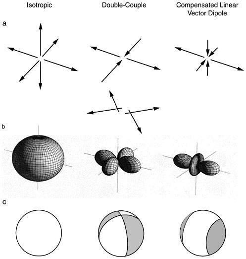
FIGURE 2.8 Graphical representations of three basic types of seismic point sources (left to right): isotropic, double couple, and compensated linear vector dipole. (a) Principal axis coordinates of equivalent force systems. (b) Compressional wave radiation patterns. (c) Curves of intersection of nodal surfaces with the focal sphere. Each of these source types is a specialization of the seismic moment tensor M. SOURCE: Modified from B.R. Julian, A.D. Miller, and G.R. Foulger, Non-double-couple earthquakes: 1. Theory, Rev. Geophys., 36, 525-549, 1998. Copyright 1998 American Geophysical Union. Modified by permission of American Geophysical Union.
physically untenable, and most of the geological community discredited Wegener’s hypothesis (46). In the 1930s, however, the South African geologist A.L. du Toit assembled an impressive set of additional geologic data that supported continental drift beginning in the Mesozoic Era, and the empirical case in its favor was further strengthened when E. Irving and S.K. Runcorn published their compilations of paleomagnetic pole positions in 1956. The paleomagnetic data indicated drifting rates on the order of centimeters per year, several orders of magnitude slower than Wegener had hypothesized. Within the next 10 years, the key elements of plate tectonics were put in place. The main conceptual breakthrough was the recognition that on a global scale, the amount of new basaltic crust generated by seafloor spreading—the bilateral separation of the seafloor along the mid-ocean ridge axis—is balanced by subduction—the thrusting of basaltic crust into the mantle at the oceanic trenches.
Seafloor Spreading and Transform Faults
Submarine mountain ranges, mapped in the 1870s, came into focus as a world-encircling system of extensional tectonics after the Second World War. Marine geologists Maurice Ewing and Bruce Heezen, based at Columbia University, mapped a narrow, nearly continuous “median valley” along the ridge crests in the Atlantic, Indian, and Antarctic Oceans, which they inferred to be a locus of active rifting and the source of the mid-ocean seismicity that Gutenberg and Richter had documented (47). In the early 1960s, Harry H. Hess of Princeton University and Robert S. Dietz of the Scripps Institution of Oceanography advanced the concept of seafloor spreading to account for observations of such phenomena as the paucity of deep-sea sediments and the tendency for oceanic islands to subside with time (48). In his famous 1960 “geopoetry” preprint, Hess noted that crustal creation at the Mid-Atlantic Ridge implies a more plausible mechanism for continental drift than the type originally envisaged by Wegener: “The continents do not plow through oceanic crust impelled by unknown forces; rather they ride passively on mantle material as it comes to the surface at the crest of the ridge and then moves laterally away from it.”
Two distinct predictions based on the theory of seafloor spreading were confirmed in 1966. The first involved the striped patterns of magnetic anomalies being mapped on the flanks of the mid-ocean ridges. In 1963, F. Vine and D. Matthews suggested that such anomalies record the reversals of the Earth’s magnetic field through remnant magnetization frozen into the oceanic rocks as they diverge and cool away from the ridge axis. These geomagnetic “tape recordings” were shown to be symmetric about this axis and consistent with the time scale of geomagnetic reversals worked out from lava flows on land; moreover, the spreading
speed measured from the magnetometer profiles in the Atlantic was found to be nearly constant and in agreement with the average opening rate obtained from the paleomagnetic data on continental rocks (49).
The second confirmation came from the study of earthquakes on the mid-ocean ridges. Horizontal displacements as large as several hundred kilometers had been documented for strike-slip faults on land, by H.W. Wellman for the Alpine fault in New Zealand and by M. Hill and T.W. Dibblee for the San Andreas (50), but even larger displacements—greater than 1000 kilometers—could be inferred from the offsets of magnetic anomalies observed across fracture zones in the Pacific Ocean (51). In a 1965 paper that laid out the basic ideas of the plate theory, the Canadian geophysicist J. Tuzo Wilson recognized that fracture zones were relics of faulting that was active only along those portions connecting two segments of a spreading ridge, which he called transform faults (52). His model implied that the sense of motion across a transform fault would be the opposite to the ridge axis offset. The seismologist Lynn Sykes of Columbia University verified this prediction in an investigation of the focal mechanisms from transform-fault earthquakes (Figure 2.9).
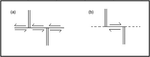
FIGURE 2.9 Two interpretations of two ridge segments offset by a fault. (a) In the pre-plate-tectonic interpretation, the two ridge segments (double lines) would have been offset in a sinistral (left-lateral) sense along the fault (solid line). Earthquakes should occur along the entire fault line. (b) According to the plate-tectonic theory, the two ridge segments were never one continuous feature. Spreading of the seafloor away from the ridges causes dextral (right-lateral) motions only along the section of the fault between the two ridge segments (the transform fault). The extensions of the faults beyond the ridge segments, the fracture zones (dashed lines), are aseismic. Earthquake observations conclusively demonstrated the validity of interpretation (b) for the mid-ocean ridges. SOURCE: Modified from L. Sykes, Mechanism of earthquakes and nature of faulting on mid-ocean ridges, J. Geophys. Res., 72, 2131-2153, 1967. Copyright 1967 American Geophysical Union. Reproduced by permission of American Geophysical Union.
Sykes’s study was facilitated by the rapidly accumulating collection of seismograms, readily available on photomicrofiche, from the new World Wide Standardized Seismographic Network (WWSSN) set up under Project Vela Uniform. These high-quality seismometers had good timing systems, fairly broad bandwidth, and a nearly uniform response to ground motions, and they were installed and permanently staffed around the world at recording sites with relatively low background noise levels (53). The high density of stations allowed smaller events to be located precisely and their focal mechanisms to be determined more rapidly and accurately than ever before. One result was much more accurate maps of global seismicity, which clearly delineated the major plate boundaries, as well as the Wadati-Benioff zones of deep seismicity (Figure 2.10).
Subduction of Oceanic Lithosphere
If the Earth’s surface area is to remain constant, then the creation of new oceanic crust at the ridge crests necessarily implies that some old crust is being recycled back into the mantle. This inference was consistent with the theories of mantle convection that attributed the volcanic arcs and linear zones of compressive orogenesis to convective downwellings (54), which David Griggs had discussed as early as 1939, calling it “a convection cell covering the whole of the Pacific basin, comprising sinking peripheral currents localizing the circum-Pacific mountains and rising currents in the center” (55). Griggs belonged to a growing group of “mobilists” who espoused the view that the Earth’s solid mantle is actively convecting like a fluid heated from below, causing large horizontal displacements of the crust, including continental drift (56). The alternative, expanding-Earth hypothesis states that the planetary radius is increasing, perhaps owing to radioactive heating or possibly to a universal decrease in gravitational strength with time, and that seafloor spreading accommodates the associated increase in surface area (57). Thus, new oceanic crust created at the spreading centers does not have to be balanced by the sinking of old crust back into the mantle.
Because of this controversy, as well as the geologic complexity of the problem, subduction was the last piece of the plate-tectonic puzzle to fall into place (58). While the system of oceanic ridges and transform faults fit neatly together in seafloor spreading, the compressional arcs and mountain belts juxtaposed all types of active faulting, which continued to baffle geologists. Benioff had pointed out the asymmetric polarity of the island arcs, correctly proposing that the deep oceanic trenches are surface expressions of giant reverse faults (59). Robert Coats used this idea to account for the initial formation of island arcs such as the Aleutians and the geochemical data bearing on the development of the
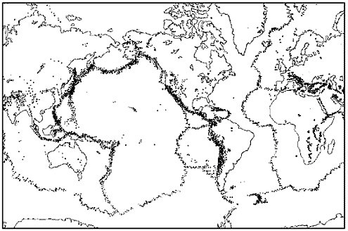
FIGURE 2.10 Locations of earthquake epicenters with body-wave magnitudes greater than 4.5 for the period 1960-1967, which incorporated the improved data of the WWSSN. Computer-generated epicenter maps such as this one first became available in about 1964 and were used to delineate the major plate boundaries and the descending slabs of cold oceanic lithosphere. Dots are epicenters reported by the U.S. Coast and Geodetic Survey. SOURCE: B.L. Isacks, J. Oliver, and L.R. Sykes, Seismology and the new global tectonics, J. Geophys. Res., 73, 5855-5899, 1968. Copyright 1968 American Geophysical Union. Reproduced by permission of American Geophysical Union.
andesitic stratovolcanoes characteristic of these arcs (60). Benioff’s model was based on several misconceptions, however, including the assumption that intermediate- and deep-focus seismicity could be explained by extrapolating trench-type reverse faulting into the mid-mantle transition zone. In fact, the focal mechanism of most earthquakes with hypocenters deeper than 70 kilometers does not agree with Benioff’s model of reverse faulting (61).
The definitive evidence for “thrust tectonics” finally arrived in the form of the great 1964 Alaska earthquake (Box 2.3). The enormous energy released in this event (~3 × 10¹⁸ joules) set the Earth to ringing like a bell and allowed precise studies of the terrestrial free oscillations, whose period might be as long as 54 minutes (62). A permanent strain of 10–8 was recorded by the Benioff strainmeter on Oahu, more than 4000 kilometers away, consistent with a fault-dislocation model of the earthquake (63). However, the high-amplitude waves drove most of the pendulum seismometers offscale (64). Moreover, field geologists could not find the fault; all ground breaks were ascribable to secondary effects. What they did observe was a systematic pattern of large vertical motions—uplifts as high as 12 meters and depressions as deep as 2.3 meters, which could easily be mapped along the rugged coastlines by observing the displacement of beaches and the stranded colonies of sessile marine organisms such as barnacles (just as Darwin had done for the 1835 Chile earthquake). By combining this pattern with the seismological and geodetic data, they inferred that the rupture represented the slippage of the Pacific Ocean crust beneath the continental margin of southern Alaska along a huge thrust fault. Geologist George Plafker concluded that “arc structures are sites of down-welling mantle convection currents and that planar seismic zones dipping beneath them mark the zone of shearing produced by downward-moving material thrust against a less mobile block of the crust and upper mantle” (65). By connecting the Alaska megathrust with the more steeply inclined plane of deeper seismicity under the Aleutian Arc, Plafker articulated one of the central tenets of plate tectonics.
Plafker’s conclusions were bolstered by more accurate sets of focal mechanisms that William Stauder and his colleagues at St. Louis University derived (66). Dan McKenzie and Robert Parker took the next major step toward completion of the plate theory in 1967, when they showed that slip vectors from Stauder’s mechanisms of Alaskan earthquakes could be combined with the azimuth of the San Andreas fault to compute a consistent pole of instantaneous rotation for the Pacific and North American plates (67). At the same time, Jason Morgan’s analysis of seafloor spreading rates and transform-fault azimuths demonstrated the global consistency of plate kinematics (68).
Clarity came with the realization that the plate is a cold mechanical
boundary layer that can act as a mechanical stress guide, capable of transmitting forces for thousands of kilometers from one boundary to another (69). The essential elements of the subduction process were brought together in a 1968 paper by seismologists Brian Isacks, Jack Oliver, and Lynn Sykes (70). In addition to obtaining improved data on earthquake locations and focal mechanisms, they delineated a dipping slab of mantle material with distinctively high seismic velocity and low attenuation, which coincided with the Wadati-Benioff planes of deep seismicity (71). They found that they could account for their results, as well as most of the other data on plate tectonics, in terms of three mechanical layers, which J. Barrell and R.A. Daly had postulated earlier in the century to explain the vertical motions associated with isostatic compensation. A cold, strong lithosphere was generated by seafloor spreading at the ridge axis and subsequent conductive cooling of the oceanic crust and upper mantle, attaining a thickness of about 100 kilometers. It slid over and eventually subducted back into a hot, weak asthenosphere. Earthquakes of the Wadati-Benioff zones were generated primarily by stresses internal to the descending slab of oceanic lithosphere when it encountered a stronger, interior mesosphere at a depth of about 700 kilometers.
Deformation of the Continents
Plate tectonics was astounding in its simplicity and the economy with which it explained so many previously disparate geological observations. In the late 1960s and 1970s, geological data were reappraised in the light of the “new global tectonics,” leading to some important extensions of the basic plate theory. However, a major problem was the obvious contrast in mechanical behavior of the oceanic and continental lithospheres. Geophysical surveys in the ocean basins revealed much narrower plate boundaries than observed on land. The volcanic rifts of active crust formation along the mid-ocean ridges were found to be only a few kilometers wide, for example, whereas volcanic activity in continental rifts could be mapped over tens to hundreds of kilometers. Similar differences were observed for transform faults; in the oceans, the active slip is confined to very narrow zones, in marked contrast to the broad belts of continental strike-slip tectonics, which often involve many distributed, interdependent fault systems. For example, only about two-thirds of the relative motion between the Pacific and North American plates turned out to be accommodated along the infamous San Andreas fault; the remainder is taken up on subsidiary faults and by oblique extension in the Basin and Range Province (see Section 3.2).
In 1970, Tanya Atwater (72) explained the geological evolution of western North America over the last 30 million years as the consequence
|
BOX 2.3 Prince William Sound, Alaska, 1964 The earthquake nucleated beneath Prince William Sound at about 5:36 p.m. on Good Friday, March 27, 1964. As the rupture spread outward, its progress to the north and east was stopped at the tectonic transition beneath the Chugach Mountains, behind the port of Valdez, Alaska, but to the southwest it continued unimpeded at 3 kilometers per second down the Alaska coastline, paralleling the axis of the Aleutian Trench for more than 700 kilometers, to beyond Kodiak Island. The district geologist of Valdez, Ralph G. Migliaccio, filed the following report:1 Within seconds of the initial tremors, it was apparent to eyewitnesses that something violent was occurring in the area of the Valdez waterfront … Men, women, and children were seen staggering around the dock, looking for something to hold onto. None had time to escape, since the failure was so sudden and violent. Some 300 feet of dock disappeared. Almost immediately a large wave rose up, smashing everything in its path…. Several people stated the wave was 30 to 40 feet high, or more…. This wave crossed the waterfront and, in some areas reached beyond McKinley Street…. Approximately 10 minutes after the initial wave receded, a second wave or surge crossed the waterfront carrying large amounts of wreckage, etc…. There followed a lull of approximately 5 or 6 hours during which time search parties were able to search the waterfront area for possible survivors. There were none. The height of the tsunami measured 9.1 meters at Valdez, but 24.2 meters at Blackstone Bay on the outer coast of the Kodiak Island group and 27.4 meters at Chenega on the Kenai Peninsula. The city of Anchorage, 100 kilometers west of the epicenter, was shielded from the big tsunami, but it experienced considerable damage, especially in the low-lying regions of unconsolidated sediment that became liquefied by the shaking. Robert B. Atwood, editor of the Anchorage Daily Times, who lived in the Turnagain Heights residential section, described his experiences during the landslide: I had just started to practice playing the trumpet when the earthquake occurred. In a few short moments it was obvious that this earthquake was no minor one…. I headed for the door … Tall trees were falling in our yard. I moved to a spot where I thought it would be safe, but, as I moved, I saw cracks appear in the earth. Pieces of the ground in jigsaw-puzzle shapes moved up and down, tilted at all angles. I tried to move away, but more appeared in every direction…. Table-top pieces of earth moved upward, standing like toadstools with great overhangs, some were turned at crazy angles. A chasm opened beneath me. I tumbled down … Then my neighbor’s house collapsed and slid into the chasm. For a time it threatened to come down on top of me, but the earth was still moving, and the chasm opened to receive the house. Migliaccio and Atwood had witnessed the second largest earthquake of the twentieth century. The plane of the rupture inferred from the dimensions of the aftershock zone was the size of Iowa (800 kilometers by 200 kilometers), and geodetic data showed that the offset along the fault averaged more than 10 meters. The product of these three numbers, which is proportional to a measure of earthquake size called the seismic moment (Equation 2.6), was thus 2000 cubic kilometers, about 100 times greater than the 1906 San Francisco earthquake. Among instrumentally recorded earthquakes, only the Chilean earthquake of 1960, which occurred in a similar tectonic setting, was bigger (by a factor of about 3). Both of these great earthquakes |
|
engendered tsunamis of large amplitude that propagated across the Pacific Ocean basin and caused damage and death thousands of kilometers from their source. Along the Oregon-California coast, 16 people were killed by the Alaska tsunami. In Crescent City, California, a series of large tsunamis inundated the harbor, beginning at four and a half hours, with the third and fourth wave causing the most damage. After the first two had struck, seven people returned to a seaside tavern to recover their valuables. Since the ocean seemed to have returned to normal, they remained to have a drink and were caught by the third wave, which killed five of them.2 |
of the North American plate overriding an extension of the East Pacific Rise along a subduction zone paralleling the West Coast. Her synthesis, which accounts for seemingly disparate events (e.g., andesitic volcanism in northern California, strike-slip faulting along the San Andreas, compressional tectonics in the Transverse Ranges, rifting in the Gulf of California) was grounded in the kinematical principles of plate tectonics (73), and her paper did much to convince geologists that the new theory was a useful framework for understanding the complexities of continental tectonics.
Convergent plate boundaries in the oceans were observed to be broader than the other boundary types, with the zone of geologic activity on the surface encompassing the trench itself, the deformed sediments and basement rocks of the forearc sequence, the volcanic arc that overlies the subducting slab, and sometimes an extending back-arc basin (74). Nevertheless, the few-hundred-kilometer widths of the ocean-ocean convergence zones did not compare with the extensive orogenic terrains that mark major continental collisions. The controlling factors were recognized to be the density and strength of the silica-rich continental crust, which are significantly lower than those of the more iron- and magnesium-rich oceanic crust and upper mantle (75). When caught between two converging plates, the weak, buoyant continental crust resists subduction and piles up into arcuate mountain belts and thickened plateaus that erode into distinctive sequences of sedimentary rock. This distributed deformation also causes metamorphism and melting of the crust, generating siliceous magmas that intrude the crust’s upper layers to form large granitic batholiths. In some instances, the redistribution of buoyancy-related stresses can lead to a reversal in the direction of subduction.
W. Hamilton used these consequences of plate tectonics to explain modern examples of mountain building, and J. Dewey and J. Bird used them to account for the geologic structures observed in ancient mountain belts (76).
Much of the early work on convergent plate boundaries interpreted mountain building in terms of two-dimensional models that consider deformations only in the vertical planes perpendicular to the strikes of the convergent zones. During a protracted continent-continent collision, however, crustal material is eventually squeezed sideways out of the collision zone along lateral systems of strike-slip faults. The best modern example is the Tethyian orogenic belt, which extends for 10,000 kilometers across the southern margin of Eurasia. At the eastern end of this belt, the convergence of the Indian subcontinent with Asia has uplifted the Himalaya, raised the great plateau of Tibet, re-elevated the Tien Shan Mountains to heights in excess of 5 kilometers, and caused deformations up to 2000 kilometers north of the Himalayan front. Earthquakes within these continental deformation zones have been frequent and dangerous.
In a series of studies, P. Molnar and P. Tapponnier explained the orientation of the major faults in southern Asia, their displacements, and the timing of key tectonic events as a consequence of the collision of the Indian continent with Asia (77). They investigated the active faulting in central Asia using photographs from the Earth Resources Technology Satellite, magnetic lineations on the ocean floor, and teleseismically determined focal mechanisms of recent earthquakes. By combining these remote-sensing observations with the plate-tectonic information, they demonstrated that strike-slip faulting has played a dominant role in the mature phase of the Himalayan collision (78).
The more diffuse nature of continental seismicity and deformation was consistent with the notion that the continental lithosphere is some-how weaker than the oceanic lithosphere, but a detailed picture required a better understanding of the mechanical properties of rocks. When subjected to differential compression at moderate temperatures and pressures, most rocks fail by brittle fracture according to the Coulomb criterion (Equation 2.1). Extensive laboratory experiments on carbonates and silicates showed that for all modes of brittle failure, the coefficient of friction µ usually lies in the range 0.6 to 0.8, with only a weak dependence on the rock type, pressure, temperature, and properties of the fault surface. This behavior has come to be known as Byerlee’s law (79), and it implies that the frictional strength of continental and oceanic lithospheres should be about the same, at least at shallow depths.
Rocks deform by ductile flow, not brittle failure, when the temperature and pressure get high enough, however, and the onset of this ductility depends on composition. Investigations of ductile flow began in 1911 with Theodore von Kármán’s triaxial tests on jacketed samples of marble.
It was found that the strength of ductile rocks decreases rapidly with increasing temperature and that their rheology approaches that of a viscous fluid. The brittle-ductile transition thus explained the plate-like behavior of the oceanic lithosphere and the fluid-like behavior of its subjacent, convecting mantle. Rock mechanics experiments further revealed that ductility sets in at lower temperatures in quartz-rich rocks than in olivine-rich rocks, typically at midcrustal depths in the continents. The ductile behavior of the lower continental crust inferred from laboratory data, which was consistent with the lack of earthquakes at these depths, thus explained the less plate-like behavior of the continents (80).
2.5 EARTHQUAKE MECHANICS
Gilbert and Reid recognized the distinction between fracture strength and frictional strength (81), and they portrayed earthquakes as frictional instabilities on two-dimensional faults in a three-dimensional elastic crust, driven to failure by slowly accumulating tectonic stresses—a view entirely consistent with plate tectonics. Although earthquakes surely involve some nonelastic, volumetric effects such as fluid flow, cracking of new rock, and the expansion of gouge zones, Gilbert and Reid’s idealization still forms the conceptual framework for much of earthquake science, both basic and applied. Nevertheless, because the friction mechanism was not obviously compatible with deep earthquakes, as described below, their view that earthquakes are frictional instabilities on faults had, by the time Wilson wrote his 1965 paper on plate tectonics, been considered and rejected by some scientists.
The Instability Problem
Deep-focus earthquakes presented a major puzzle. Seismologists had found that the deepest events, 600 to 700 kilometers below the surface, are shear failures just like shallow-focus earthquakes and that the decrease in apparent shear stress during these events is on the order of 10 megapascals, about the same size as the stress drops estimated for shallow shocks. According to a Coulomb criterion (Equation 2.1), the shear stress needed to induce frictional failure on a fault should be comparable to the lithostatic pressure, which reaches 2500 megapascals in zones of deep seismicity. Shear stresses of this magnitude are impossibly high, and if the stress drop approximates the absolute stress, as most seismologists believe, they would conflict with the observations (82).
Furthermore, if earthquakes result from a frictional instability, the motion across a fault must at some point be accelerated by a drop in the frictional resistance. A spontaneous rupture like an earthquake thus re-
quires some type of strain weakening, but the rock deformations observed in the laboratory at high pressure and temperature tended to display strain hardening during ductile creep. In a classic 1960 treatise Rock Deformation, D. Griggs and J. Handin (83) concluded that the old theory of earthquakes’ originating by ordinary fracture with sudden loss of cohesion was invalid for deep earthquakes, although they did note that extremely high fluid pressures at depth could validate that same mechanism they presumed to hold for shallow events.
A renewed impetus was given to the frictional explanation in 1966, when W.F. Brace and Byerlee demonstrated that the well-known engineering phenomenon of stick-slip also occurs in geologic materials (84). Experimenting on samples with preexisting fault surfaces, they observed that the stress drops in the laboratory slip events were only a small fraction of the total stress. This implies that the stress drops during crustal earthquakes could be much smaller than the rock strength, eliminating the major seismological discrepancy. Subsequent experiments at the Massachusetts Institute of Technology found a transition from stick-slip behavior to ductile creep at about 350°C (85). Stick-slip instabilities thus matched the properties of earthquakes in the upper continental crust, which were usually confined above this brittle-ductile transition, although this could not explain the deeper shocks in subduction zones. In addition, Brace and Byerlee’s work focused theoretical attention on how frictional instabilities depend on the elastic properties of the testing machine or fault system (86).
During the next decade, the servo-controlled testing machine was developed, in which the load levels and strain rates were precisely regulated, so that the postfailure part of the load-deformation curve in brittle materials could be followed without the stick-slip instabilities encountered with less stiff machines (87). Several new aspects of rock friction were investigated, including memory effects and dilatancy (88). The subsequent development of high-precision double-direct-shear and rotary-shear devices (89) allowed detailed measurements of friction for a wide range of materials under variable sliding conditions. This work documented three interrelated phenomena:
-
Static friction µs depends on the history of sliding and increases logarithmically with the time two surfaces are held in stationary contact (90).
-
Under steady-state sliding, the dynamic friction µd depends logarithmically on the slip rate V, with a coefficient that can be either positive (velocity strengthening) or negative (velocity weakening) (91).
-
When a slipping interface is subjected to a sudden change in the loading velocity, the frictional properties evolve to new values over a
-
characteristic slipping distance Dc, measured in microns and interpreted as the slip necessary to renew the microscopic contacts between the two rough surfaces (92).
During 1979 to 1983, J.H. Dieterich and A.L. Ruina (93) integrated these experimental results into a unified constitutive theory in which the slip rate V appears explicitly in the friction equation and the frictional strength evolves with a characteristic time set by the mean lifetime Dc/V of the surface contacts. The behavioral transition of Brace and Byerlee around 350 degrees, from stick-slip to creep, was interpreted by Tse and Rice (94) as a transition from rate weakening to rate strengthening in the crust and was shown to allow models of earthquake sequences in a crustal strike-slip fault to reproduce primary features inferred for natural events, such as the depth range of seismic slip and rapid after-slip below.
Scaling Relations
According to the dislocation model of earthquakes, slip on a small planar fault is equivalent to a double-couple force system, where the total moment M0 of each couple is proportional to the product of the fault’s area A and its average slip u:
(2.6)
The constant of proportionality G is the elastic shear modulus, a measure of the resistance to shear deformation of the rock mass containing the fault, which can be estimated from the shear-wave velocity. For waves that are large compared with the dislocation, the amplitude of radiation increases in proportion with M0, so that this static seismic moment can be measured directly from seismograms. K. Aki made the first determination of seismic moment from the long-period surface waves of the 1964 Niigata earthquake (95). Many subsequent studies have demonstrated a consistent relationship between seismic moment and the various magnitude scales developed from the Richter standard; the results can be expressed as a general moment magnitude MW of the form
(2.7)
Equation 2.7 defines a unified magnitude scale (96) based on a physical measure of earthquake size. Calculating magnitude from seismic moment avoids the saturation effects of other magnitude estimates, and this procedure became the seismological standard for determining earthquake size. The 1960 Chile earthquake had the largest moment of any known seismic event, 2 × 10²³ newton-meters, corresponding to Mw = 9.5 (Table 2.1).
TABLE 2.1 Size Measures of Some Important Earthquakes
|
Date |
Location |
MS |
MW |
M0 (1018 N-m) |
|
April 18, 1906 |
San Francisco |
8.25 |
8.0 |
1,000 |
|
Sept. 1, 1923 |
Kanto, Japan |
8.2 |
7.9 |
850 |
|
Nov. 4, 1952 |
Kamchatka |
8.25 |
9.0 |
35,000 |
|
March 9, 1957 |
Aleutian Islands |
8.25 |
9.1 |
58,500 |
|
May 22, 1960 |
Chile |
8.3 |
9.5 |
200,000 |
|
March 25, 1964 |
Alaska |
8.4 |
9.2 |
82,000 |
|
June 16, 1964 |
Niigata, Japan |
7.5 |
7.6 |
300 |
|
Feb. 4, 1965 |
Aleutian Islands |
7.75 |
8.7 |
12,500 |
|
May 31, 1970 |
Peru |
7.4 |
8.0 |
1,000 |
|
Feb. 4, 1975 |
Haicheng, China |
7.4 |
6.9 |
31 |
|
July 28, 1976 |
Tangshan, China |
7.9 |
7.6 |
280 |
|
Aug. 19, 1977 |
Sumba |
7.9 |
8.3 |
3,590 |
|
Oct. 28, 1983 |
Borah Peak |
7.3 |
6.9 |
31 |
|
Sept. 19, 1985 |
Mexico |
8.1 |
8.0 |
1,100 |
|
Oct. 18, 1989 |
Loma Prieta |
7.1 |
6.9 |
27 |
|
June 28, 1992 |
Landers |
7.5 |
7.3 |
110 |
|
Jan. 17, 1994 |
Northridge |
6.6 |
6.7 |
12 |
|
June 9, 1994 |
Bolvia |
7.0a |
8.2 |
2,630 |
|
Jan. 16, 1995 |
Hyogo-ken Nanbu, Japan |
6.8 |
6.9 |
24 |
|
Aug. 17, 1999 |
Izmit, Turkey |
7.8 |
7.4 |
242 |
|
Sept. 20, 1999 |
Chi-Chi, Taiwan |
7.7 |
7.6 |
340 |
|
Oct. 16, 1999 |
Hector Mine |
7.4 |
7.1 |
60 |
|
Jan. 13, 2001 |
El Salvador |
7.8 |
7.7 |
460 |
|
Jan. 26, 2001 |
Bhuj, India |
8.0 |
7.6 |
340 |
|
NOTE: All events are shallow except Bolivia, which had a focal depth of 657 km. Moment magnitude MW computed from seismic moment M0 via Equation 2.7. aBody-wave magnitude. SOURCES: U.S. Geological Survey and Harvard University. |
||||
Unless otherwise noted, all magnitudes given throughout the remainder of this report are moment magnitudes.
Beginning in the 1950s, arrays of temporary seismic stations were deployed to study the aftershocks of large earthquakes. Aftershocks are caused by subsidiary faulting from stress concentrations produced by the main shock, owing to inhomogeneities in fault slippage and heterogeneities in the properties of the nearby rocks. Omori’s work on the 1891 Nobi earthquake had demonstrated that the frequency of aftershocks decayed inversely with the time following the main shock (97). In its modern form, “Omori’s law” states that the aftershock frequency obeys a power law of the form
n(t) = A(t + c)–p, (2.8)
where t is the time following the main shock and c and p are parameters of the aftershock sequence. Aftershock surveys confirmed that p is near unity (usually slightly greater) for most sequences. They also showed that the aftershock zone approximated the area of faulting inferred from geologic and geodetic measurements (98).
With independent information about rupture area A from aftershock, geologic, or geodetic information, Equation 2.6 can be solved for the average fault displacement u. Aki obtained a value of about 4 meters for the 1964 Niigata earthquake by this method, consistent with echo-sounding surveys of the submarine fault scarp. A second method derived fault dimensions from the “corner frequency” of the seismic radiation spectrum, an observable value inversely proportional to the rupture duration (99). Corner frequencies were easily measurable from regional and teleseismic data and could be converted to fault lengths by assuming an average rupture velocity (100). Using this procedure, seismologists estimated the source dimensions for a much larger set of events, paving the way for global studies of the stress changes during earthquakes.
For an equidimensional rupture surface, the ratio
Seismic Source Studies
Seismic moment measures the static difference between initial and final states of a fault, not what happens during the rupture. To investigate the dynamics of rupture process, seismologists had to tackle the difficult problem of determining the space-time distribution of faulting during an earthquake from its radiated seismic energy. In the 1960s, a simple kinematic dislocation model with uniform slip and rupture speed was devel-
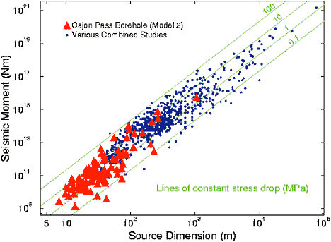
FIGURE 2.11 Seismic moment as a function of source dimension. When plotted on a log-log scale, the diagonal lines (slope = 3) indicate M0 ~ r3 and denote constant stress drop. Note that measurements of the static stress drop vary as the cube of the corner frequency, a sensitivity that contributes to substantial scatter in ?s for individual events. The value cited is based on a numerical study of rupture dynamics (R. Madariaga, Dynamics of an expanding circular fault, Bull. Seis. Soc. Am., 66, 639-666, 1976) and applies to shear waves radiated by a circular, cohesionless fault that stops suddenly around a circular periphery. Using a particular estimate for the source radius in terms of the corner frequency fc yields ?s ˜ 47M0(fc/ß)3. SOURCE: R.E. Abercrombie, Earthquake source scaling relationships from –1 to 5 ML using seismograms recorded at 2.5-km depth, J. Geophys. Res.,100, 24,015-24,036, 1995. Copyright 1995 American Geophysical Union. Reproduced by permission of American Geophysical Union.
oped by N. Haskell to understand the energy radiation from an earthquake and the spectral structure of a seismic source (104). Haskell’s model predicted that the frequency spectrum of an earthquake source is flat at low frequency and falls off as ?–2 at high frequency, where ? is the angular frequency. This simple model (generally called the omega-squared model) was extended to accommodate the much more complex kinematics of real seismic faulting, described stochastically (105), and it was found
to approximate the spectral observations rather well, especially for small earthquakes.
The orientation of an elementary dislocation depends on two directions, the normal direction to the fault plane and the slip direction within this plane, so that the double-couple for a dislocation source is described by a three-dimensional, second-order moment tensorM proportional to M0 (106). By 1970, it was recognized that the seismic moment tensor can be generalized to include an ideal (spherically symmetrical) explosion and another type of seismic source called a compensated linear vector dipole (CLVD). A CLVD mechanism was invoked as a plausible model for seismic sources with cylindrical symmetry, such as magma-injection events, ring-dike faulting, and some intermediate- and deep-focus events (Figure 2.8) (107).
The Stress Paradox
Plate tectonics accounted for the orientation of the stress field on simple plate boundaries, which could be classified according to Anderson’s three principal types of faulting: divergent boundaries (normal faults), transform boundaries (strike-slip faults), and convergent boundaries (reverse faults). The stress orientations mapped on plate interiors using a variety of indicators—wellbore breakouts, volcanic alignments, and earthquake focal mechanisms—were generally found to be coherent over distances of 400 to 4000 kilometers and to match the predictions of intraplate stress from dynamic models of plate motions (108). This behavior implies that the spatial localization of intraplate seismicity primarily reflects the concentration of strain in zones of crustal weakness (109). Explaining the orientation of crustal stresses was a major success for the new field of geodynamics.
About 1970, a major debate erupted over the magnitude of the stress responsible for crustal earthquakes. Byerlee’s law implies that the shear stress required to initiate frictional slip should be at least 100 megapascals, an order of magnitude greater than most seismic stress drops (110). The stresses measured during deep drilling generally agree with these predictions. If the average stresses were this large, however, the heat generated by earthquakes along major plate boundaries would greatly exceed the radiated seismic energy and the heat flowing out of the crust along active fault zones should be very high. Attempts to measure a heat flow anomaly on the San Andreas fault found no evidence of a peak (111). The puzzle of fault stress levels was further complicated as data became available in the middle to late 1980s on principal stress orientations in the crust near the San Andreas (112); the maximum stress direction was found to be steeply inclined to the fault trace and to re-
solve more stress onto faults at angles to the trace of the San Andreas fault than onto the San Andreas fault itself. These results, as well as data on subduction interfaces and oceanic transform faults, suggest that most plate-bounding faults operate at low overall driving stress, on the order of 20 megapascals or less. Various explanations have been put forward (113)—intrinsically weak materials in the fault zones, high fluid pore pressures, or dynamical processes that lower frictional resistance such as wave-generated decreases in normal stress during rupture—but the stress paradox remains a major unsolved problem.
2.6 EARTHQUAKE PREDICTION
Earthquake prediction is commonly defined as specifying the location, magnitude, and time of an impending earthquake within specified ranges. Earthquake predictions are customarily classified into long term (decades to centuries), intermediate term (months to decades), and short term (seconds to weeks). The following discussion is divided the same way, but the classification is not definitive because many proposed methods span the time boundaries. Because some predictions might be satisfied by chance, seismologists almost inevitably invoke probabilities to evaluate the success of an earthquake prediction. Many seismologists distinguish forecasts, which may involve relatively low probabilities, from predictions, which involve high enough probabilities to justify exceptional policy or scientific responses. This distinction, which is adopted here, implies that predictions refer to times when the earthquake probability is temporarily much higher than normal for a given region and magnitude range. Forecasts might or might not involve temporal variations. Even if they involve only estimates of the “normal” probability, long-term forecasts can be extremely useful for input to seismic hazard calculations and for decisions about building, retrofitting, insuring, and so forth. A clear statement of the target magnitude is crucial to evaluating a prediction because small earthquakes are so much more frequent than large ones. A prediction of a moment magnitude (M) 6 earthquake for a given region and time might be very bold, while a prediction of an M 5 event could easily be satisfied by chance.
Long-Term Forecasts
G.K. Gilbert issued what may have been the first scientifically based, long-term earthquake forecast in his 1883 letter to the Salt Lake City Tribune (114), in which he articulated the practical consequences of his field work along the seismically active Wasatch Front:
Any locality on the fault line of a large mountain range, which has been exempt from earthquake for a long time, is by so much nearer to the date of recurrence…. Continuous as are the fault-scarps at the base of the Wasatch, there is one place where they are conspicuously absent, and that place is close to [Salt Lake City]…. The rational explanation of their absence is that a very long time has elapsed since their last renewal. In this period the earth strain has slowly been increasing, and some day it will overcome the friction, lift the mountains a few feet, and reenact on a more fearful scale the [1872] catastrophe of Owens Valley.
So far, Gilbert’s forecast for Salt Lake City has not been fulfilled (115). H.F. Reid developed Gilbert’s “principle of alternation” into a quantitative theory of earthquake forecasting. In his 1910 report for the Lawson Commission, he wrote: “As strains always precede the rupture and as the strains are sufficiently great to be easily detected before rupture occurs (116), … it is merely necessary to devise a method of determining the existence of strains; and the rupture will in general occur … where the strains are the greatest.” He suggested that the time of the next major earthquake along that segment of the San Andreas fault could be estimated by establishing a line of piers at 1-kilometer spacing perpendicular to the fault and observing their positions “from time to time.” When “the surface becomes strained through an angle of 1/2000, we should expect a strong shock.” Reid noted that this prediction scheme relied on measurements commencing when the fault was in an “unstrained condition,” which he presumed was the case following the 1906 earthquake (117).
The Gilbert-Reid forecast hypothesis—the idea that a large earthquake is due when the critical strain from the last large event has been recovered by steady tectonic motions—is the basis for the seismic-gap method. In its simplest form, this hypothesis asserts that a particular fault segment fails in a quasi-periodic series of earthquakes with a characteristic size and average recurrence interval. This interval can be estimated either from known dates of past characteristic earthquakes or from D/V, the ratio of the average slip in a characteristic quake to the long-term slip rate on the fault. A seismic gap is a fault segment that has not ruptured in a characteristic earthquake for a time longer than T. A. Imamura identified Sagami Bay, off Tokyo, as a seismic gap, and his prediction of an impeding rupture was satisfied by the disastrous Kanto earthquake of 1923 (118). Fedotov is generally credited with the first modern description of the seismic-gap method, publishing a map in 1965 showing where large earthquakes should be expected (119). His predictions were promptly satisfied by three major events (Tokachi-Oki, 1968; southern Kuriles, 1969; central Kamchatka, 1971).
Forecasting large earthquakes using the seismic-gap principle looked fairly straightforward in the early 1970s. Plate tectonics had established a
precise kinematic framework for estimating the rates of geological deformation across plate boundaries, specifying a deformation budget that could be balanced against historic seismic activity. For example, Sykes divided the amount of co-seismic slip during the 1957, 1964, and 1965 Aleutian Trench earthquakes by the rate of relative motion between the North American and Pacific plates, obtaining recurrence intervals of a century or so for each of the three segments (120). Self-consistent models of the relative plate motions were derived from global data sets that included seafloor magnetic anomalies tied to the precise magnetic reversal time scale (121), allowing Sykes’s calculation to be repeated for many of the major plate boundaries. Sykes and his colleagues produced maps in 1973 and 1979 showing plate boundary segments with high, medium, and low seismic potential based on the recent occurrence of large earthquakes (122) and published a more refined forecast in 1991 (123) (Figure 2.12).
While some form of the Gutenberg-Richter distribution is observed for almost all regions, Schwartz and Coppersmith (124) proposed that many individual faults, or segments of faults, behave quite differently. They proposed that most of the slip on a fault segment is released in large “characteristic” earthquakes having, for a given segment, similar magnitude, rupture area, and average displacement. It follows that characteristic earthquakes must be much more frequent, relative to smaller and larger earthquakes, than the Gutenberg-Richter relationship would predict. Wesnousky and colleagues (125) argue that earthquakes in a region obey the Gutenberg-Richter relationship because the fault segments there have a power-law distribution.
Characteristic earthquakes have profound implications for earthquake physics and hazards. For example, characteristic earthquakes can be counted confidently, and their average recurrence time would be an important measure of seismic hazard. The time of the last one would start a seismic clock, by which the probability of another such earthquake could be estimated. For Gutenberg-Richter earthquakes, the simple clock concept does not apply: for any magnitude of quake, there are many more earthquakes just slightly smaller but no different in character. The characteristic earthquake model has strong intuitive appeal, but the size of the characteristic earthquake and the excess frequencies of such events have been difficult to demonstrate experimentally (126).
The seismic-gap method met limited success as a basis for earthquake forecasting (127). Attempts to use it as a general tool were frustrated by the difficulty of specifying characteristic magnitudes and the lack of historical records needed to estimate the recurrence interval T. Moreover, the practical utility of the seismic-gap hypothesis was compromised by the intrinsic irregularity of the earthquake process and the tendency of earthquakes to cluster in space and time. The Gilbert-Reid idea that a
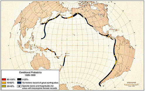
FIGURE 2.12 Circum-Pacific plate boundary segments with high, medium, and low seismic potential. Colors indicate time-dependent probability of the recurrence of either a large or a great shallow plate earthquake within a specified segment during the interval 1989 to 1999, conditional upon the event not having occurred prior to 1989. SOURCE: Modified from S.P. Nishenko, Circum-Pacific seismic potential: 1989-1999, Pure Appl. Geophys., 135, 169-259, 1991.
given fault segment will fail periodically assumes that the stress drop in successive earthquakes and the rate of stress accumulation between earthquakes are both constant. However, stick-slip experiments in well-controlled laboratory settings show variations in the time between slip events, which had incomplete and irregular stress drops, indicating variations in either the initial (rupture) stress or the final (postearthquake) stress, or both. Shimizaki and Nakata (128) discussed two special cases (Figure 2.13). In the “time-predictable” model, the initial stress is the same for successive large earthquakes, but the final stress varies. This implies that the time until the next earthquake is proportional to the stress drop, or average slip, in the previous event (Tn = Dn–1/V), while the size of the next quake Dn is not predictable. In the “slip-predictable” model, the initial stress varies from event to event, but the final stress is the same. This implies that the slip in the next earthquake is proportional to the time since the last one (Dn = TnV), while the time Tn is not predictable. Shimazaki and Nakata found that the Holocene uplift data for several well-studied sites in Japan were consistent with a time-predictable model of the largest events.
Japanese seismologists and geologists have long been at the forefront of earthquake prediction studies, and their government has sponsored the world’s largest and best-funded research programs on earthquake phenomena (129). One area of intense concern is the so-called Tokai seismic gap, southwest of Mt. Fuji (Box 2.4). This region is threatened by a
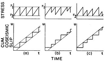
FIGURE 2.13 Schematic models of earthquake recurrence intervals for constant tectonic loading rates. (a) Constant stress drop, showing strictly periodic behavior (modified Reid model). (b) Variable stress drop, constant failure stress (time-predictable model). (c) Variable stress drop, constant final stress (slip-predictable model). SOURCE: K. Shimazaki and T. Nakata, Time-predictable recurrence model for large earthquakes, Geophys. Res. Lett., 7, 279-282, 1980. Copyright 1980 American Geophysical Union. Reproduced by permission of American Geophysical Union.
|
BOX 2.4 The Tokai Seismic Gap Large earthquakes have repeatedly occurred in the Nankai Trough along the southwestern coast of Japan. The sequence during the past 500 years includes large (M ~ 8) earthquakes in 1498, 1605, 1707, 1854, and 1944-1946, with an approximate interval of about 120 years. In the early 1970s, several Japanese seismologists noticed that the 1944-1946 events were somewhat smaller than the 1854 and 1707 earthquakes, and they suggested that this rupture did not reach the northeastern part of the Nankai Trough, called the Suruga Trough. Given the historical evidence that the rupture of both the 1854 and the 1707 events extended all the way to the Suruga Trough, they concluded that this portion of the plate boundary, which became known as the “Tokai seismic gap,” has the potential for a magnitude-8 earthquake in the near future.1 In 1978, the Japanese government introduced the Large-Scale Earthquake Countermeasures Act and embarked on an extensive project to monitor the Tokai gap. Many institutions deployed geophysical and other instrumentation, and very detailed plans for emergency relief efforts were made. This program specified the procedures for short-term prediction. When some anomaly is observed by the monitoring network, a special evaluation committee comprising technical experts is to decide whether it is a precursor for the predicted Tokai earthquake or not. If the anomaly is identified as a precursor, a large-scale emergency operation is to be initiated by the local and central governments. A detailed plan for this activity has been laid out as part of the prediction experiment. After more than 23 years since the project began, no anomaly that requires initiation of the preplanned emergency operation has been detected. The chair of the Tokai evaluation committee, Professor K. Mogi, resigned in 1997, expressing doubts about the ability of the committee to perform its expected short-term prediction function, and the new chair, M. Mizoue, has voiced similar concerns. Also, a report released in 1997 by the Geodesy Council of Japan concluded that a technical basis for short-term prediction of the kind required by the Countermeasures Act does not currently exist in Japan, and that the time frame for establishing such a capability is not known.2 |
potentially large earthquake on the thrust fault of the Suruga Trough, known to have ruptured in the great earthquakes of 1707 and 1854 and thought to be ripe for failure at any time. So far, the expected Tokai earthquake has not occurred. Many seismologists now agree that accurate forecasts are difficult even for plate boundaries such as this one that have seemingly regular historical sequences of earthquakes.
The Parkfield, California, earthquake prediction (130), arguably the boldest widely endorsed by the seismological community, was also based on the seismic gap theory. Moderate earthquakes of about M 6 on the San Andreas fault near Parkfield were recorded instrumentally in 1922, 1934, and 1966, and pre-instrumental data revealed that similar-size earthquakes occurred in 1857, 1881, and 1901. The regular recurrence of Parkfield events at an average interval of about 22-years and the similarity of the foreshock pattern in 1934 and 1966 led to the hypothesis that these events were characteristic earthquakes, breaking the same segment of the San Andreas with about the same slip. Estimates of the recurrence time from the ratio of earthquake displacement to fault slip agreed with the 22-year value above. Based on these and other data, the U.S. Geological Survey (USGS) issued an official prediction of an earthquake of about M 6 in about 1988, on an identified segment of the San Andreas, with 95 percent probability before the beginning of 1993. While the size and location of the predicted event were not precisely specified, no earthquake matching the description has occurred as of January 1, 2002 (131).
The seismic-gap model forms the basis of many other forecasts. Most involve low enough probabilities that they are not predictions by the usual definition, and they cannot yet be confirmed or rejected by available data. A notable example was the 1988 “Working Group Report” (132). The authors postulated specific segments of the San Andreas and other major strike-slip faults in California, and then tabulated characteristic magnitudes, average recurrence times, and 30-year probabilities for each segment. They estimated a 66 percent probability of at least one large characteristic earthquake on the four southern segments of the San Andreas fault before 2018, with a similar chance for northern California.
The 1989 Loma Prieta earthquake (M 6.9) occurred in an area where several seismologists (and the Working Group) had made long-term or intermediate-term forecasts of a large earthquake (133). It occurred near the southern end of the 1906 rupture, a segment of the San Andreas to which the Working Group assigned a 30-year probability of 30 percent. The earthquake was considered a successful forecast, especially as it happened just two years after the report was published. On the other hand success by chance cannot be ruled out, and the earthquake did not exactly match the forecasts (134).
Intermediate-Term Prediction
Intermediate-term prediction efforts are generally based on recognizing geophysical anomalies that might signal a state of near-critical stress approaching the breaking point. Apparent anomalies have been observed in small earthquake occurrence: accelerated strain or uplift; changes in
the gravity field, magnetic field, electrical resistivity, water flow, groundwater chemistry, atmospheric chemistry; and many other parameters that might be sensitive to stress, cracks in rock, or changes in the frictional properties of rocks. The literature is extensive (135); only a few examples are discussed here.
A logical successor to the seismic-gap model is the hypothesis that earthquake occurrence is accelerated or decelerated by stress increments from previous earthquakes. One version of this hypothesis is the stress shadow model—that the occurrence of large earthquakes reduces the stress in certain neighborhoods about their rupture zones, thus decreasing the likelihood of both large and small earthquakes there until the stress recovers (136). The stress model differs from the seismic-gap model in that it applies not just to a fault segment, but to the region surrounding it. Furthermore, because stress is a tensor, it may encourage some faults and discourage others. In some regions near a ruptured fault segment, the stress is actually increased, offering an explanation for seismic clustering. At present, the model offers a good retrospective explanation for many earthquake sequences, but it has not been implemented as a testable prediction hypotheses because the stress pattern depends on details of the previous rupture, fault geometry, stress-strain properties of the crust, possible fluid flow in response to earthquake stress increments, and other properties that are very difficult to measure in sufficient detail.
Seismicity patterns are the basis of many prediction attempts, in part because reliable seismicity data are widely available. Mogi described a sequence of events that many feel can be used to identify stages in a repeatable seismic cycle involving large earthquakes (137). In this model a large earthquake may be followed by aftershocks of decreasing frequency, a lengthy period of quiescence, an increase of seismicity about the future rupture zone, a second intermediate-term quiescence, a period for foreshock activity, a third short-term quiescence, and finally the “big one.” Any of the stages may be missing. This behavior formed the basis of an apparently successful prediction of the M 7.7 Oaxaca, Mexico, earthquake of 1978 (138). Unfortunately, there are no agreed-on definitions of the various phases that can be applied uniformly, nor has there been a comprehensive test of how Mogi’s model works in general (139).
Computerized pattern recognition has been applied in several experiments to recognize the signs of readiness for large earthquakes. V. Keilis-Borok and Russian colleagues have developed an algorithm known as “M8” that scans a global catalog for changes in the earthquake rate, the ratio of large to small earthquakes, the vigor and duration of aftershock sequences, and other diagnostics within predefined circles in seismically active areas (140). They report significant success in predicting which circles are more likely to have large earthquakes (141). Since 1999, they
have made six-month advance predictions for magnitude thresholds 7.5 and 8.0 accessible on their web page (142), and fully prospective statistical tests will be possible in the near future.
Short-Term Prediction
The “Holy Grail” of earthquake science has always been short-term prediction—anticipating the time, place, and size of a large earthquake in a window narrow and reliable enough to prepare for its effects (143). However, interest in the possibility of detecting earthquake precursors grew as new technologies were developed to monitor the crustal environment with increasing sensitivity. In the year following the destructive 1964 Alaskan earthquake, a select committee of the White House Office of Science and Technology issued a report called Earthquake Prediction: A Proposal for a Ten Year Program of Research, which called for a national program of research focused on this goal (144).
Optimism about the feasibility of short-term prediction was height-ened in the mid-1970s by the apparent successes of empirical prediction schemes and the plausibility of physical process models, such as dilatancy diffusion. Laboratory studies had measured dilatant behavior in rocks prior to failure, caused by pervasive microcracking. Dilatancy creates measurable strain, changes the material properties, and increases the permeability of the samples (145). Field evidence for such effects came from the Garm region of the former U.S.S.R., where Soviet seismologists had identified changes in the ratio of shear and compressional velocities, VS/VP, as precursors to some moderate earthquakes (146). Positive results on VS/VP precursors were also reported in the United States (147). These observations prompted refinements of the dilatancy diffusion model and a wider search for related precursors.
A reported prediction of an M 7.3 earthquake in Haicheng, China, is widely regarded as the single most successful earthquake prediction. An international team that visited China shortly after the quake (148) reported that the region had already been subject to an intermediate-term earthquake forecast based on seismicity patterns, magnetic anomalies, and other geophysical data. Accelerating seismic activity (Figure 2.14) and rapid changes in the flow from local water wells prompted Chinese officials to issue a short-term prediction and to evacuate thousands of unsafe buildings. At 7:36 p.m. (local time) on February 4, 1975, less than 24 hours after the evacuation began, the main shock destroyed 90 percent of the city. Chinese officials stated that because of the evacuation the number of casualties was extremely low for such an earthquake. This reported success stimulated great optimism in the earthquake prediction community, but it did not signal a widespread breakthrough in predic-
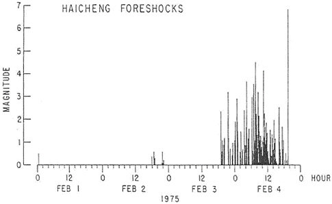
FIGURE 2.14 Plot of the magnitude versus time occurrence of the larger foreshocks of the Haicheng earthquake sequence, February 1-4, 1975. As indicated by the final large event, the earthquake occurred at 7:36 p.m. on February 4. SOURCE: P. Molnar, T. Hanks, A. Nur, B. Raleigh, F. Wu, J. Savage, C. Scholz, H. Craig, R. Turner, and G. Bennett, Prediction of the Haicheng earthquake, Eos, Trans. Am. Geophys. Union, 58, 236-272, 1977. Copyright 1977 American Geophysical Union. Reproduced by permission of American Geophysical Union.
tion science. First, the foreshock series and hydrologic precursors were highly unusual, and similar phenomena have not been recognized before other large earthquakes. Second, the Chinese issued many false alarms, so the possibility of success by chance cannot confidently be rejected. Unfortunately, complete records of predictions and consequent actions are not accessible. The apparent triumph of the Haicheng prediction was soon overshadowed by disaster in July 1976, when a devastating (M 7.8) quake struck the Chinese city of Tangshan, resulting in the deaths of at least 240,000 people—one of the highest earthquake death tolls in recorded history. Although this area was also being monitored extensively, the disaster was not predicted.
Nevertheless, many prominent geophysicists were convinced that systematic short-term prediction was feasible and that the challenge remaining was to deploy adequate instrumentation to find and measure precursors of earthquake warnings (149). By 1976 a distinguished group of earthquake scientists convened by the National Research Council was willing to state (150):
The Panel unanimously believes that reliable earthquake prediction is an achievable goal. We will probably predict an earthquake of at least magnitude 5 in California within the next five years in a scientifically sound way and with a sufficiently small space and time uncertainty to allow public acceptance and effective response.
In 1977, the U.S. government initiated the National Earthquake Hazards Reduction Program (Appendix A) to provide “data adequate for the design of an operational system that could predict accurately the time, place, magnitude, and physical effects of earthquakes.” The USGS has the responsibility for issuing a prediction (statement that an earthquake will occur), whereas state and local officials have the responsibility for issuing a warning (recommendation or order to take defensive action).
The observational and theoretical basis for prediction soon began to unravel. Careful, repeated measurements showed that the purported Vs/ Vp anomalies were not reproducible (151). At the same time, questions arose about the uniqueness of a posteriori reports of geodetic, geochemical, and electromagnetic precursors. Finally, theoretical models (152) incorporating laboratory rock dilatancy, microcracking, and fluid flow gave no support to the hypothesized Vs/Vp time history. By the end of the 1970s, most of the originally proposed precursors were recognized to be of limited value for short-term earthquake prediction (153).
Attention shifted in the 1980s to searching for transient slip precursors preceding large earthquakes. The hypothesis that such behavior might occur was based on the results of detailed laboratory sliding experiments and model simulations (154) and on qualitative field observations prior to an M 6 earthquake on the San Andreas fault near Parkfield, California (155). The preseismic slip observed under laboratory conditions was very subtle, but theoretical calculations suggested that under favorable conditions it might be observable in the field, provided that the critical slip distance Dc observed in the lab studies scaled to a larger size on natural faults.
To investigate these issues, the USGS launched a focused earthquake prediction experiment near Parkfield, in anticipation that an M 6 earthquake was imminent. Geodetic instrumentation, strainmeters, and tiltmeters were deployed to make continuous, precise measurements of crustal strains near the expected epicenter (Figure 2.15). The strain data were anticipated to place much stricter bounds on any premonitory slip. The predicted moderate earthquake has not occurred, so it is premature to evaluate the success of the search for short-term precursors. Nonetheless, the Parkfield experiment has contributed valuable data that improve our understanding of faults, deformation, and earthquakes.
After more than a century of intense research, no reliable method for short-term earthquake prediction has been demonstrated, and there is no
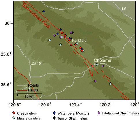
FIGURE 2.15 The network of crustal deformation instruments along the San Andreas fault maintained by the U.S. Geological Survey near Parkfield, California. SOURCE: U.S. Geological Survey.
guarantee that reliable short-term prediction will ever be feasible. At best, only a few earthquake “precursors” have been identified, and their applicability to other locations and earthquakes is questionable. Research continues on a broad range of proposed techniques for short-term prediction, as does vigorous debate on its promise (156). Most seismologists now agree that the difficulties of earthquake prediction were previously underestimated and that basic understanding of the earthquake process must precede prediction.
2.7 EARTHQUAKE ENGINEERING
The 1891 Nobi earthquake killed more than 7000 people and caused substantial damage to modern brick construction in the Nagoya region (157). Milne noted the extreme variability of ground shaking over short
distances and reported that “buildings on soft ground … suffer more than those on hard ground.” He laid the foundation for the development of codes regulating building construction by emphasizing that “we must construct, not simply to resist vertical stresses, but carefully consider effects due to movements applied more or less in horizontal directions” (158). Milne’s conclusions were echoed in California following the 1906 San Francisco earthquake. J.C. Branner, a Stanford professor of geology on the Lawson Commission, supervised a detailed study of more than 1000 houses in San Mateo and Burlingame, and he noted that the local site response had a major influence on the level of damage: “The intensity of the shock was less on the hills than on the flat, in spite of the fact that the houses in the hills were nearer the fault line.” Throughout California, the damage patterns were well correlated with the type of structure and building materials (159).
Early Building Codes
The first attempt to quantify the “earthquake design force” was made after the 1908 Messina-Reggio earthquake in southern Italy, which killed more than 83,000. In a report to the Italian government, M. Panetti, a professor of applied mechanics in Turin, recommended that new buildings be designed to withstand horizontal forces proportional to the vertical load (160). The Japanese engineer Toshikata Sano independently developed in 1915 the idea of a lateral design force V proportional to the building’s weight W. This relationship can be written as V = CW, where C is a lateral force coefficient, expressed as some percentage of gravity (%g, where g = 9.8 m/s2). The first official implementation of Sano’s criterion was the specification C = 10 percent of gravity, issued as a part of the 1924 Japanese Urban Building Law Enforcement Regulations in response to the destruction caused by the great 1923 Kanto earthquake (161). In California, the Santa Barbara earthquake of 1925 motivated several communities to adopt codes with C as high as 20 percent of gravity. The first edition of the U.S. Uniform Building Code (UBC), published in 1927, also adopted Sano’s criterion, allowing for variations in C depending on the region and foundation material (162). For building foundations on soft soil in earthquake-prone regions, the UBC’s optional provisions corresponded to a lateral force coefficient equal to the Japanese value.
Measurement of Strong Ground Motions
By 1930, networks of permanent seismic observatories allowed the location and analysis of large earthquakes anywhere on the globe. However, the sensitive instruments could not register the strong (high-amplitude)
ground motions close to large earthquakes, the primary cause of damage and loss of life, and were of little value to engineers. Consequently, engineers were forced to estimate the magnitude of the near-source ground accelerations from damage effects (e.g., overturned objects). The American engineer John Freeman voiced the frustration felt by many of his colleagues when he wrote in 1930 (163):
The American structural engineer possesses no reliable accurate data about form, amplitude or acceleration of the motion of the earth during a great earthquake…. Notwithstanding there are upward of fifty seismograph stations in the country and an indefinitely large number of seismologists, professional and amateur; their measurements of earthquake motion have been all outside of the areas so strongly shaken as to wreck buildings.
Japanese seismologists were the first to attempt to obtain these data systematically. They began to record strong ground motions using long-period seismometers with little or no magnification, and by the 1930s, the development of broader-band, triggered devices allowed accurate measurement of the waves most destructive to buildings, those with shorter period and therefore higher acceleration. The Long Beach earthquake of 1933 was the first large event to be recorded by these improved strong-motion seismometers, several of which had been installed in the Los Angeles region just nine months before the earthquake. This new equipment recorded a peak acceleration of 29 percent of gravity on the vertical component and 20 percent of gravity on the horizontal component. The widespread damage caused by the 1933 Long Beach earthquake (Figure 2.16) spurred legislation for stricter building codes throughout California. One month after the event, the California Assembly passed the Field Act, which effectively prohibited masonry construction in public schools by instituting a lateral force requirement equivalent to 10 percent of the sum of the dead load (weight of the building) and the live load (weight of the contents). The Riley Act, also enacted in 1933, required all buildings in California to resist lateral forces of at least 2 percent of the total vertical design load. On September 6, 1933, the city of Los Angeles passed a law requiring a lateral force of 8 percent of the dead load plus 4 percent of the live load.
The success of the Long Beach recording can be credited to the Seismological Field Survey, which was established in California by the U.S. Department of Commerce at the urging of Freeman. A limited number of strong-motion instruments were deployed (164). One such instrument, located on the concrete block foundation of the Imperial Valley Irrigation District building in El Centro, recorded the next significant California event, the 1940 Imperial Valley earthquake (M 7.1). A peak horizontal
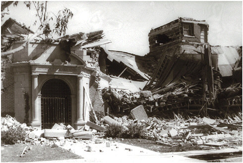
FIGURE 2.16 Jefferson Junior High School destroyed in the Long Beach earthquake. The Field Act, passed one month after the earthquake, prohibited this type of masonry construction for schools in California. SOURCE: Steinbrugge Collection, Earthquake Engineering Research Center, University of California, Berkeley. Photograph by Harold M. Engle.
acceleration of 33 percent of gravity was recorded at a distance of approximately 10 kilometers from the fault rupture. For the next 25 years, this was the largest measured ground acceleration, establishing the El Centro record as the de facto standard for earthquake engineering in the United States and Japan (Figure 2.17).
Response Spectra for Structural Analysis
Both the Long Beach and the El Centro data influenced the development of seismic safety provisions in building codes. However, the impact of seismometry on earthquake engineering was limited by the lack of data from a wider distribution of earthquakes, as well as by computational difficulties in performing a quantitative analysis of ground shaking and its effect on structures. Simplified techniques for structural analysis, such as H. Cross’s moment-distribution method and K. Muto’s D-value method, had been encoded in tables and figures by the early 1930s (165).
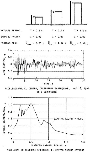
FIGURE 2.17 Accelerogram of the 1940 Imperial Valley earthquake (center panel), schematic representation of the response of a series of single degree-of-freedom oscillators having different natural periods (top), and their application to the construction of the response spectrum (bottom panel). SOURCE: H.B. Seed and I.M. Idriss, Ground Motions and Soil Liquefaction During Earthquakes, Earthquake Engineering Research Institute, Engineering Monograph on Earthquake Criteria, Structural Design, and Strong Motion Records 5, El Cerrito, Calif., 134 pp., 1982.
The advent of analog computers in the 1940s provided the first simulations of structural vibrations induced by the recorded ground motions (166) and allowed the automation of strong-motion spectral analysis (167). These early calculations showed that the spectra of earthquake accelerations are similar to “white noise” over a limited range of frequencies, a pivotal observation in the study of earthquake source processes. However, the immediate implication for earthquake engineering was the lack of a “dominant ground period” that might be destructive to particular structures (168). Without a characteristic frequency, earthquake engineering was recognized to be complex, requiring a comprehensive analysis of coupled vibrations between earthquakes and structures. George Housner outlined the issues in 1947:
In engineering seismology, the response of structures to strong-motion earthquakes is of particular interest…. During an earthquake a structure is subjected to vibratory excitation by a ground motion which is to a high degree erratic and unpredictable…. Furthermore, the average structure, together with the ground upon which it stands, is an exceedingly complex system from the viewpoint of vibration theory. It is apparent the problem divides itself into two parts; first a determination of the characteristics of strong motion earthquakes, and second a determination of the characteristics of structures subjected to earthquakes.
Following an earlier suggestion by M.A. Biot, Housner put forward the concept of the response spectrum, the maximum response induced by ground motion in single degree-of-freedom oscillators (“buildings”) with different natural periods but the same degree of internal damping (usually selected to be 5 percent) (169) (Figure 2.17). At shorter periods the maximum induced acceleration exceeds the recorded ground acceleration, whereas for longer periods it is less. When multiplied by the effective mass of a building, the response spectrum acceleration constrains the lateral force that a building must sustain during an earthquake. Computing response spectra over a wide range of frequencies using data from a wide range of earthquakes significantly improved understanding of the damage potential of strong motion.
Building Code Improvements Since 1950
The availability of strong-motion data began to transform earthquake engineering from a practice based on pseudostatic force criteria to a science grounded in an understanding of the complex coupling between ground motions and building vibrations. By the 1950s, strong-motion records were combined with response spectral analysis to demonstrate that structures can amplify the free-field accelerations (recorded on open
ground). To approximate this dynamic behavior, a committee of the American Society of Civil Engineers and the Structural Engineers Association of Northern California proposed in 1952 that the lateral force requirement be revised to vary inversely with the building’s fundamental period of vibration (C ~ T–1). With only a handful of strong-motion recordings available at the time, the decrease in the response spectral accelerations with period remained uncertain. Particular attention was focused on the band from 0.5 to 5.0 seconds, which includes the fundamental periods of vibration for most midrise to high-rise buildings as well as many other large structures.
The lateral force coefficient was recast in the 1961 UBC with a weaker (inverse cubed root) dependence on the response period: C ~ ZKT–1/3. This version introduced a seismic zone factor Z that represented the variability of the seismic hazard throughout the United States and a structural factor K that depended on building type and accounted for its dynamic response. The parameters were chosen to reproduce as well as possible the response spectral accelerations measured in previous earthquakes, which were still sparse. The uncertainties in the empirical coefficients remained high, but the form of the lateral force requirement did establish a firm connection between strong-motion measurements and the requirements of earthquake engineering.
The dearth of strong-motion data ended when the San Fernando earthquake (M 6.6) struck the Los Angeles region on February 9, 1971. It subjected a community of more than 400,000 people to ground accelerations greater than 20 percent of gravity and triggered in excess of 200 strong-motion recorders, more than doubling the size of the database. San Fernando provided the first well-resolved picture of the temporal and spatial variability of ground shaking during an earthquake (170). Short-period (0.1-second) accelerations varied widely, even among nearby sites with similar geologic conditions, while long-period (10-second) displacements were coherent over tens of kilometers (171). More important, this earthquake demonstrated that the ground motions could substantially exceed the maximum values observed in previous events. A strong-motion instrument on an abutment of the Pacoima Dam, 3 kilometers above the fault plane, recorded a sharp, high-amplitude (100-centimeter-per-second) velocity pulse in the first three seconds of the earthquake, as the rupture front passed under the dam (Figure 2.18). Four seconds later, after the rupture had broken the surface 5 kilometers away in the San Fernando Valley, the Pacoima instrument recorded an acceleration pulse exceeding 1.2 gravity in the horizontal plane. This value more than doubled the highest previously observed peak ground acceleration (PGA), measured during the 1966 Parkfield earthquake (M 5.5) on the San Andreas fault (172). The short acceleration pulse observed at Pacoima Dam
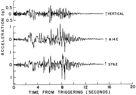
FIGURE 2.18 Three component records of acceleration, velocity, and displacement from the Pacoima Dam record of the San Fernando earthquake. The horizontal instruments are approximately parallel and perpendicular to the horizontal component of the rupture (N14E and S76E, respectively) and show accelerations exceeding 1 g. SOURCE: D.M. Boore and M.D. Zoback, Two dimensional kinematic fault modeling of the Pacoima Dam strong-motion recordings of February 9, 1971, San Fernando Earthquake, Bull. Seis. Soc. Am.,64, 555-570, 1974. Copyright Seismological Society of America.
engendered much discussion regarding the utility of PGA as a measure of seismic hazard. This pulse did not make a significant contribution to the overall response spectra values, except at the shortest periods (173), and when the data from all available earthquakes were considered, PGA was only weakly correlated with the size of the earthquake (174). From these and subsequent studies, it became clear that the PGA was not necessarily the best determinant of seismic hazard to structures; other characteristics—such as the response spectrum ordinates, anisotropic motions, and the occurrence of intense, low-frequency velocity pulses—were found to be more important.
After the 1971 San Fernando earthquake, policy makers tried to update building codes in light of the large amount of data on ground motion
and building response collected from this urban event. The wealth of strong-motion data also prompted a 1976 revision to the UBC, which modified the period scaling in the lateral force equation from T–1/3 to T–1/2 and introduced a factor S based on local soil type. The newly formed Applied Technology Council (ATC) organized, with funding from the National Science Foundation (NSF) and the National Bureau of Standards, a national effort to develop a model seismic code. More than 100 professionals who volunteered for the work were organized into 22 committees. In a comprehensive report published in 1978 (175), the ATC proposed a more physically based lateral force coefficient of the form C ~ AvSR–1T–2/3, where Av is the effective peak ground velocity-related acceleration coefficient, S is a site-dependent soil factor, and R is a “response modification factor” dependent on the structure type. At shorter periods, this expression was replaced by a limiting value proportional to the effective peak acceleration coefficient Aa. The report also provides the first contoured maps of the ground-motion parameters Aa and Av, derived from a probabilistic seismic hazard analysis conducted by the USGS.
Strong-motion data from a number of earthquakes, as well as laboratory test data and results of numerical site response models, demonstrated the need to modify the soil factor S to reflect nonlinear site response. The National Center for Earthquake Engineering Research, which NSF established in 1986, led the revision, recommending two sets of amplitude-dependent, site amplification factors derived for six site geology classifications. The factors were first incorporated in the 1994 National Earthquake Hazard Reduction Program (NEHRP) seismic provisions and then into the 1997 UBC.
Strong-motion data from the 1994 Northridge, California (M 6.7), and 1995 Kobe, Japan (M 6.9), earthquakes confirmed observations from several previous earthquakes that motions recorded close to the fault rupture had distinct pulse-like characteristics, which were not represented in the code’s lateral force equation. The effect of these pulse motions was approximated by introducing near-fault factors into the lateral force equation. A single factor N was first introduced in the base isolation section of the 1994 UBC. This representation was replaced by two near-fault factors Na and Nv in the lateral force provisions of the 1997 UBC lateral force requirement. The Na factor was applied to the short-period, constant-acceleration portion of the design response spectrum, whereas the Nv factor was applied to the intermediate- and long-period constant-velocity portion, where the base shear is proportional to T–1. Interestingly, after a 36-year absence, the T–1 proportionality was reintroduced in the 1997 UBC in part because it was judged to be a more accurate representation of the spectral character of earthquake ground motion (176).
Attenuation Relationships
Engineers wanted the scattered ground-motion observations reduced to simple empirical relationships that practitioners could apply, and the derivation of these relationships became a central focus of engineering seismology. A measure of shaking intensity was chosen (typically peak ground acceleration or velocity), and the observed variation of this intensity measure was factored into source, path, and site effects by identifying one or more independent control variables—typically, source magnitude, path distance, and site condition (e.g., soil or rock)—and fitting the observations with parameterized curves. The magnitude dependence or scaling and the fall-off of strong-motion amplitude with epicentral distance were together called the attenuation relation.
Lack of data precluded plotting PGA as a function of magnitude and epicentral distance until the 1960s. Figure 2.19 shows an attenuation relationship obtained from the strong-motion data for the 1979 Imperial Valley earthquake. The dispersion in the data resulted in a relative standard deviation of about 50 percent, which was typical. Other relationships described the site response in terms of the correlation between intensity measures and soil and rock conditions, including allowance for nonlinear soil behavior as a function of shaking intensity (Figure 2.20).
As the use of the response spectrum method increased, it became necessary to develop techniques to predict not only the PGA (equivalent to the response spectral value at zero period) but also the response spectra of earthquakes that might occur in the future. This was done initially by developing a library of response spectral shapes that varied with earthquake magnitude and soil conditions; the selected shape was anchored to a peak acceleration obtained from a set of attenuation relationships, each of which predicted the spectral acceleration at a specific period. Eventually, response spectra were computed directly from ground-motion attenuation relationships.
Seismic Hazard Analysis
By the 1960s, growing strong-motion databases and scientific understanding enabled site-specific seismic hazard assessments incorporating information about the length and distance of neighboring faults, the history of seismicity, and empirical predictions of ground-motion intensity for events of specified magnitude at specified distances. For major facilities in the western United States, in particular nuclear power plants such as San Onofre and Diablo Canyon (177), seismic hazard assessment focused on the maximum magnitude that each fault could produce, its closest distance to the site, and the PGA for these events. PGA was then the
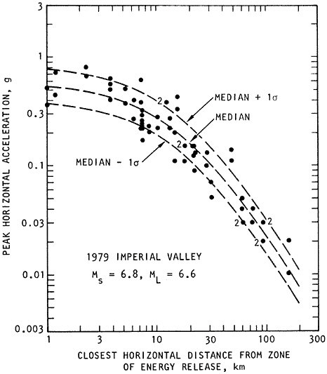
FIGURE 2.19 Recorded peak accelerations of the 1979 Imperial Valley earthquake and an attenuation relation that has been fit to the data. SOURCE: H.B. Seed and I.M. Idriss, Ground Motions and Soil Liquefaction During Earthquakes, Earthquake Engineering Research Institute, Engineering Monograph on Earthquake Criteria, Structural Design, and Strong Motion Records 5, El Cerrito, Calif., 134 pp., 1982.
primary scalar measure of ground-motion intensity for use in structural analysis and design. Typically PGA was used to scale a standard response spectral shape or, if the engineer requested more detailed ground-motion information, “standard” accelerograms, such as the El Centro record from the 1940 Imperial Valley earthquake. The basic motivation for these pro-
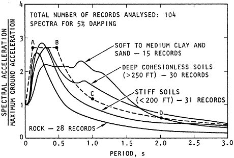
FIGURE 2.20 Average response spectral shapes for different soil categories derived from strong-motion recordings. The response spectral shapes are normalized to peak acceleration, which is equivalent to zero-period acceleration. The dashed line ABCD indicates a simplified response spectral shape for rock and stiff soil sites that was developed for use in building codes. SOURCE: H.B. Seed and I.M. Idriss, Ground Motions and Soil Liquefaction During Earthquakes, Earthquake Engineering Research Institute, Engineering Monograph on Earthquake Criteria, Structural Design, and Strong Motion Records 5, El Cerrito, Calif., 134 pp., 1982.
cedures was to identify a conservative or bounding value for the maximum potential threat at a specific site. These procedures are now referred to as deterministic to distinguish them from the probabilistic techniques that followed.
The deterministic methods of seismic hazard analysis developed for seismically active sites in California and other western states were unsuited to the tectonically stable environment of the eastern United States, where likely earthquake sources were largely unknown and strong-motion data had not yet been recorded. Therefore, a modified deterministic analysis had to be developed for the some 100 nuclear power plants east of the Rocky Mountains, based on “seismotectonic zones” developed from historic seismic activity and geologic trends. Application of these methods relies heavily on the judgment of scientists and engineers. Although the historical record for this analysis is comparatively long (about 300 years), estimates of past earthquake magnitude were limited to verbal
accounts of earthquake effects translated into the 12 levels of the Modified Mercalli Intensity (MMI) scale (see endnote 27). The largest historic event in the zone became the basis for establishing the maximum event, typically the largest MMI or one-half intensity unit larger, depending on circumstances (e.g., nature of the facility, design rules, safety factors adopted by the engineers). The largest event in each zone was then presumed to occur as close to the site as the seismotectonic zone boundary permitted, except for events in the zone that contained the site, where a minimum separation was adopted to reflect the improbability of an event occurring very close to the site. Lacking sufficient ground-motion data, engineering seismologists used MMI data to develop attenuation relations, calibrating MMI to PGA with data from the western United States.
Probabilistic seismic hazard analysis (PSHA) was developed to characterize and integrate several effectively random elements of earthquake occurrence and ground-motion forecasting. The method uses probabilistic analysis to combine the seismic potential from several threatening faults, or spatially distributed across source zones characterized for each by an assumed frequency-magnitude distribution, to obtain an estimate of the total hazard, defined as the mean annual rate at which the chosen intensity measure, such as PGA, will exceed some specified threshold at a prescribed site (178). For each fault, the contribution to hazard was derived from a convolution of the mean annual rate of earthquakes with the probability that the shaking intensity will be exceeded for an event of specified magnitude. The method allows for assumed distributions of event location (e.g., randomly along the fault or within a region) and for variance about the predicted ground motions due to natural variability. The final result for a site is a hazard curve, a plot of mean annual frequency of exceedance at a specified intensity level.
By the late 1970s, the PSHA method had been tested and its application was growing throughout engineering seismology. As with the deterministic method, the practical application of PSHA at a specific site requires professional judgments based on local data and experience. In response to these difficulties, uncertainties in the model parameters associated with the limits of scientific information (e.g., in earthquake catalogs, fault locations, ground-motion prediction) are quantified and propagated through PSHA to produce quantitative confidence bounds on the resulting hazard curves. The objective of the hazard curve is to capture the randomness or “aleatory uncertainty” inherent in the forecasting of future events, while the confidence bounds reflect the current limits on professional knowledge, or “epistemic uncertainty,” in such forecasts. Figure 2.21 presents an example of the analysis for a site in the San Francisco Bay area.
PSHA relies on a wider range of scientific information than deterministic analysis. It also satisfies modern engineering requirements for a
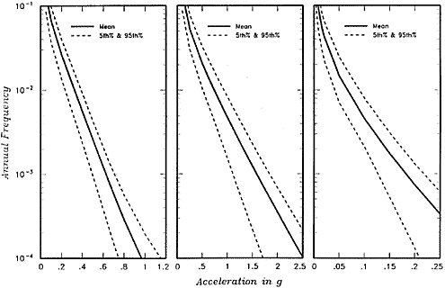
FIGURE 2.21 Mean estimate and 5/95 percent confidence bounds on the mean annual frequency hazard curves for the east end of the San Mateo-Hayward Bridge, San Francisco Bay area, California, for PGA and 5 percent damped spectral accelerations at oscillator periods of 0.3 and 3.0 seconds. SOURCE: Geomatrix Consultants, Inc., Seismic Ground Motion Study for San Mateo-Hayward Bridge, Final Report , prepared for CALTRANS, Division of Structures, Oakland, Calif,, 234 pp. + 6 appendixes, February 1993.
probabilistic definition of risk. Common engineering practice evolved to define a design ground-motion in terms of a specified frequency of exceedance. This value is lower (i.e., increases the design requirements) for facilities where structural failure involves more severe consequences.
Seismic Hazard Maps
Seismic hazard analysis for buildings, highway overpasses, and smaller structures has traditionally relied on design values mapped nationally or regionally. Early maps were quite crude owing to the typical building-code practice of using only four or five discrete zones with large relative differences (factor of 2) in ground-motion level. At first, the zones were drawn largely to reflect historic seismicity. For example, the first seismic probability map for the United States, distributed in 1948 by the U.S. Coast and Geodetic Survey (USCGS), simply used the locations of historic earthquakes and divided the country into four zones ranging from no expected damage to major damage (179). This basis led to under-stated earthquake hazards in the Pacific Northwest, the eastern Basin and Range Province, and other places with long recurrence intervals. The work was revised in 1958 and 1959 when Charles Richter published several maps based on the seismic regionalization technique that Soviet seismologists had developed in the 1940s (180). Richter also relied on historic seismicity and employed MMI as the intensity measure. In 1969, S.T. Algermission of the USCGS produced a national map with maximum MMI values from historic earthquakes contoured as zones, along with a table and map of earthquake recurrence rates. The maximum-intensity map was the basis for the UBC national zoning map published in 1970.
Several years later, Algermissen and coworkers at the USGS, using PSHA, repeated the national mapping (181). They produced a seismic hazard curve at each point on a grid; the PGA was calculated for a 10 percent probability of exceedance in 50 years; and these values were contoured to produce a national seismic hazard map. The maps provided quantitative estimates of the expected shaking (excluding site effects). They also furnished a compelling visual representation of the relative seismic hazard among different locations in the United States and were the basis for national building code zoning maps in 1979. The USGS updated the national seismic hazard maps in 1982, 1990, 1991, 1994, and 1996, incorporating new knowledge on earthquake sources and seismic-wave propagation. The 1991 maps were the first to display probabilistic values of response spectral ordinates and were published in the NEHRP Recommended Provisions for Seismic Regulations for New Buildings. The 1996 maps implemented a completely new PSHA methodology and provide the basis for the probabilistic portion of the seismic design guidelines in
the 1997 and 2000 NEHRP Provisions and the 2000 International Building Code. These seismic hazard maps are also used in seismic provisions for highway bridge design, the International Residential Code, and many other applications.
Challenges Ahead
Establishing building codes, developing attenuation relationships and performing seismic hazard analysis are all examples of earthquake engineering activities that have helped quantify and reduce the threat posed by earthquakes; however, recent large earthquakes make it clear that significant challenges remain. For example, the 1995 Hyogo-ken Nanbu earthquake (Box 2.5, Figures 2.22 and 2.23) devastated the city of Kobe, in Japan—one of the most earthquake-prepared countries in the world. That this earthquake caused such tremendous damage and loss of life indicates
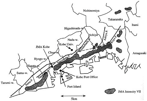
FIGURE 2.22 Kobe-Osaka region, annotated with major faults and geographic reference points, including inferred rupture during the 1995 earthquake and damage belt. SOURCE: H. Kawase, The cause of the damage belt in Kobe: “The basin-edge effect,” constructive interference of the direct s-wave with the basin-induced diffracted/Rayleigh waves, Seis. Res. Lett., 67, 25-34, 1996. Copyright Seismological Society of America.
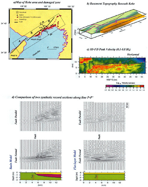
FIGURE 2.23 Numerical simulations of basin-edge effects in the 1995 Hyogo-ken Nanbu earthquake. SOURCE: A. Pitarka, K. Irikura, T. Iwata, and H. Sekiguchi, Three-dimensional simulation of the near-fault ground motion for the 1995 Hyogo-ken Nanbu (Kobe), Japan, earthquake, Bull. Seis. Soc. Am., 88, 428-440, 1998. Copyright Seismological Society of America.
|
BOX 2.5 Kobe, Japan, 1995 The official name of the M 6.9 earthquake that struck Kobe, Japan, on January 17, 1995 is Hyogo-ken Nanbu (Southern Hyogo Prefecture). It killed at least 5500 people, injured more than 26,000, and caused immense destruction throughout a metropolis of 1.5 million people. One-fifth of its inhabitants were left homeless, and more than 100,000 buildings were destroyed. The total direct economic loss has been estimated as high as $200 billion.1 The Japanese call an earthquake with an epicenter directly under a city a chokkagata. History has demonstrated repeatedly that a direct hit on an urban center can be terribly destructive; for example, an earlier chokkagata wiped out the city of Tangshan, China, in 1976, killing at least 240,000. Nevertheless, given the rigorous Japanese building codes and disaster preparations, the extreme devastation to the city center was surprising. In contrast, the 1994 Northridge earthquake was of comparable size (M 6.7, only a factor of 2 smaller in seismic moment), and occurred in a densely populated region (the San Fernando Valley of California) but killed only 57 people and caused about $20 billion in damages.2 The high losses in the Hyogo-ken Nanbu earthquake can be attributed to at least four independent factors:
|
|
that reducing, or even containing, the vulnerabilities to future earthquakes as urbanization of earthquake-prone regions increases, constitutes a major and continuing challenge for earthquake science and engineering.
NOTES
|
|
data set was good enough that it could be used eight decades later to model this event as a blind thrust (R. Chander, Interpretation of observed ground level changes due to the 1905 Kangra earthquake, northern Himalaya, Tectonophysics, 149, 289-298, 1988). |
|
10. |
During the first half of the nineteenth century, most geologists viewed vertical uplift by magmatic processes as the main cause of mountain building. The importance of horizontal compression was recognized in the context of Appalachian tectonics by W.B. Rogers and H.D. Rogers (On the physical structure of the Appalachian chain, as exemplifying the laws which have regulated the elevation of great mountain chains, generally, Assoc. Am. Geol. Rep., 1, 474-531, 1843) and championed by the supporters of Élie de Beaumont’s theory (1829) that the Earth was cooling and therefore contracting. The latter included the great Austrian geologist, Eduard Suess, whose five-volume treatise Das Antlitz der Erde (The Face of the Earth) (Freytag, Leipzig, 158 pp., 1909) synthesized global tectonics in terms of the contraction hypothesis. |
|
11. |
E.M. Anderson, Dynamics of faulting, Trans. Geol. Soc. Edinburgh,8, 387-402, 1905. He further developed his ideas in a monograph The Dynamics of Faulting and Dyke Formation with Application to Britain (2nd ed., Oliver & Boyd, Edinburgh, 206 pp., 1951). |
|
12. |
M.K. Hubbert and W.W. Rubey, Mechanics of fluid-filled porous solids and its application to overthrust faulting, 1: Role of fluid pressure in mechanics of overthrust faulting, Geol. Soc. Am. Bull., 70, 115-166, 1959. In soil mechanics, the use of effective normal stress in the Coulomb criterion is sometimes called Terzaghi’s principle, after the engineer who first articulated the concept (K. Terzaghi, Stress conditions for the failure of saturated concrete and rock, Proc. Am. Soc. Test. Mat., 45, 777-792, 1945). The historical development of the mechanical theory of faulting has been summarized by M.K. Hubbert in Mechanical Behavior of Crustal Rocks: the Handin Volume (N.L. Carter, M. Friedman, J.M. Logan, and D.W. Sterns, eds., Geophys. Mono. 24, American Geophysical Union, Washington, D.C., pp. 1-9, 1981). |
|
13. |
The hydrostatic pressure at depth h is the pressure of a water column that deep, whereas the lithostatic pressure is the full weight of the overlying rocks; the latter is greater than the former by the rock-to-water density ratio, a factor of about 2.7. |
|
14. |
State Earthquake Investigation Commission, The California Earthquake of April 18, 1906, Publication 87, vol. I, Carnegie Institution of Washington, 451 pp., 1908, and vol. II, with Atlas (by H.F. Reid), 192 pp., 1910; reprinted 1969. The Lawson Commission submitted a preliminary report almost immediately, on May 31, 1906, but no state or federal funds were available to continue the investigation, so that most of the research following the event had to be underwritten by a private organization, the Carnegie Institution of Washington. |
|
15. |
The correlation between earthquake damage and “made ground” was noted 38 years before the 1906 earthquake when San Francisco’s financial district was badly damaged in the 1868 Hayward earthquake. The 1906 quake caused extensive damage to the same area. |
|
16. |
The State Earthquake Investigation Commission reports on the 1906 earthquake have been the principal source of data for the study of strong ground motions by D.M. Boore (Strong-motion recordings of the California earthquake of April 18, 1906, Bull. Seis. Soc. Am., 67, 561-577, 1977), the reconstruction of the space-time sequence of rupture by D.J. Wald, H. Kanamori, D.V. Helmberger, and T.H. Heaton (Source study of the 1906 San Francisco earthquake, Bull. Seis. Soc. Am., 83, 981-1019, 1993), and the recent reinterpretation of the geodetic measurements by W. Thatcher, G. Marshall, and M. Lisowski (Resolution of fault slip along the 470-kilometer-long rupture of the great 1906 San Francisco earthquake and its implications, J. Geophys. Res., 102, 5353-5367, 1997). These studies, which applied state-of-the-art techniques to old data, form the basis for the reconstruction of the faulting events outlined in Box 2.2. |
|
135. |
For a recent compilation, including long-, intermediate-, and short-term prediction, see the conference proceedings introduced by L. Knopoff, Earthquake prediction: The scientific challenge, Proc. Natl. Acad. Sci., 93, 3719-3720, 1996. Articles by many other authors follow in sequence. For a brief, cautiously skeptical review see D.L. Turcotte, Earthquake prediction, Ann. Rev. Earth Planet. Sci., 19, 263-281, 1991. For a detailed, negative assessment of the history of earthquake prediction research, see R.J. Geller, Earthquake prediction: A critical review, Geophys. J. Int., 131, 425-450, 1997. |
|
136. |
J. Deng and L. Sykes, Evolution of the stress field in southern California and triggering of moderate-size earthquakes; A 200-year perspective, J. Geophys. Res., 102, 9859-9886, 1997; R.A. Harris and R.W. Simpson, Stress relaxation shadows and the suppression of earthquakes; Some examples from California and their possible uses for earthquake hazard estimates, Seis. Res. Lett., 67, 40, 1996; R.A. Harris and R.W. Simpson, Suppression of large earthquakes by stress shadows; A comparison of Coulomb and rate-and-state failure, J. Geophys. Res., 103, 24,439-24,451, 1998. |
|
137. |
K. Mogi, Earthquake Prediction, Academic Press, Tokyo, 355 pp., 1985. Mogi’s “do-nut” hypothesis is summarized succinctly in C. Scholz, The Mechanics of Earthquakes and Faulting, Cambridge University Press, New York, pp. 340-343, 1990. |
|
138. |
M. Ohtake, T. Matumoto, and G. Latham, Seismicity gap near Oaxaca, southern Mexico, as a probable precursor to a large earthquake, Pure Appl. Geophys., 113, 375-385, 1977. Further details are given in M. Ohtake, T. Matumoto, and G. Latham, Evaluation of the forecast of the 1978 Oaxaca, southern Mexico earthquake based on a precursory seismic quiescence, in Earthquake Prediction—An International Review, D. Simpson and P. Richards, eds., American Geophysical Union, Maurice Ewing Series 4, Washington, D.C., pp. 53-62, 1981. Interpretation of the success of the prediction and the reality of the precursor is complicated by a global change in earthquake recording because some large seismic networks were closed in 1967. For more details, see R.E. Habermann, Precursory seismic quiescence: Past, present, and future, Pure Appl. Geophys., 126, 277-318, 1988. |
|
139. |
A comprehensive test requires a complete record of successes and failures for predictions made using well-defined and consistent methods. Otherwise, the likelihood of success by chance cannot be evaluated. |
|
140. |
V.I. Kieilis Borok, and V.G. Kossobokov, Premonitory activation of seismic flow: Algorithm M8, Phys. Earth Planet. Int., 61, 73-83, 1990. |
|
141. |
J.H. Healy, V.G. Kossobokov, and J.W. Dewey, A Test to Evaluate the Earthquake Prediction Algorithm M8, U.S. Geological Survey Open-File Report 92-401, Denver, Colo., 23 pp. + 6 appendixes, 1992; V.G. Kossobokov, L.L. Romashkova, V.I. Keilis-Borok, and J.H. Healy, Testing earthquake prediction algorithms: Statistically significant advance prediction of the largest earthquakes in the circum-Pacific, 1992-1997, Phys. Earth Planet. Int., 111, 187-196, 1999. |
|
142. |
See <http://www.mitp.ru/predictions.html>. A password is needed to access predictions for the current six-month time interval. |
|
143. |
John Milne noted this quest in his treatise Earthquakes and Other Earth Movements (D. Appelton and Company, New York, pp. 301 and 310, 1899): “Ever since seismology has been studied, one of the chief aims of its students has been to discover some means which could enable them to foretell the coming of an earthquake, and the attempts which have been made by workers in various countries to correlate these occurrences with other well-marked phenomena may be regarded as attempts in this direction.” Milne himself proposed short-term prediction schemes based on measurements of ground deformation and associated phenomena, such as disturbances in the local electromagnetic field. “As our knowledge of earth movements, and their attendant phenomena, increases there is little doubt that laws will be gradually formulated and in the future, as telluric disturbances increase, a large black ball gradually ascending a staff |


