
APPENDIX TO CHAPTER 7
DOMINICI et al. (2000) used a two-stage Bayesian model to pool dose-response information across a relatively large number of studies. The first stage of their analysis estimated dose-response slopes from each study, adjusting for various confounding factors measured for each study. The second stage involved fitting a hierarchical Bayesian model to the estimates obtained at the first stage. The approach is heuristically appealing and is in fact similar to the ad-hoc two-stage algorithm that was often used to fit linear growth curve models before the advent of programs such as SAS PROC MIXED (see, for example, Laird 1990). As noted by Dominici et al., the approach approximates a fully Bayesian analysis on the original data. The authors justified this approximation by (1) empirically checking this approximation for their particular application and (2) pointing to theoretical justification for the approximation given by Daniels and Dass (1998). A two-stage analysis along the same lines is attractive in the context of MeHg for several reasons. First, the approach is natural in settings in which the original study-specific data are unavailable. That is, one can simply fit the second stage of the model to published summary measures (i.e., dose-response slopes and corresponding standard errors) from each study. Second, the approach easily extends to the case of multiple outcomes, because outcome within a study simply represents an additional level in the hierarchical model. As discussed in the chapter, data available to the committee included estimated BMDs and BMDLs computed for each of the individual outcomes assessed for the Faroe Islands, Seychelles, and
New Zealand studies (see Table 7-3). One approach might be to apply the hierarchical analysis directly to the estimated BMDs, although the committee felt it appropriate to apply the analysis to the inverse BMDs instead. One advantage of working with the inverse BMDs is that very large and undefined values are transformed to zero. Working with the inverse BMDs also has some theoretical justification, because in the context of a linear model, the estimated BMD is simply a constant divided by the estimated dose-response slope (see Equation 7-1).
To describe the committee's approach in more detail, it is useful to define some notation. Let ![]() be the inverse of the BMD estimated for the jth outcome, j = 1, . . . Ji, within study, i = 1, . . . I. The corresponding standard errors,
be the inverse of the BMD estimated for the jth outcome, j = 1, . . . Ji, within study, i = 1, . . . I. The corresponding standard errors, ![]() , can be estimated by subtracting
, can be estimated by subtracting ![]() from the inverse of the BMDL and then dividing by 1.64. The hierarchical model can be expressed as
from the inverse of the BMDL and then dividing by 1.64. The hierarchical model can be expressed as
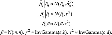
where a, b, c, d, m, and n are chosen so that the priors are all relatively noninformative. In other words, we assume that the true inverse BMDs for each outcome are normally distributed around a study-specific mean value and that these study-specific values are in turn normally distributed around an overall mean. We fit the hierarchical model using the BUGS (Bayesian inference Using Gibbs Sampling) software package (Spiegelhalter et al. 1996). The product of the analysis is a series of simulated distributions of the various random variables defined in the model. Applying an inverse transformation again converts those results to yield estimates of the distribution of the quantities of interest, namely, BMDs. In addition to providing an estimate of distribution of true BMDs corresponding to different outcomes from different studies, the output from the program allows computation of so-called posterior estimates of the true BMDs, given the observed values. The advantage
of working with the posterior estimates instead of the original values is that they have removed some of the random variation inherent in the observed estimates. The “smoothed BMDs” referred to in Chapter 7 and also in Figure 7-3 are posterior estimates.
Because the method proposed here is new and exploratory in nature, the committee does not recommend it as the primary approach to the MeHg risk assessment at the present time. Indeed, there are a number of questions associated with the approach that would require further exploration before it could be used as the basis of a definitive analysis. For example, one concern is the relatively small number of studies (three) available for the MeHg study. The Dominici et al (2000) analysis involved a relatively large number of studies, and therefore, does not have the same concern.
REFERENCES
Daniels, M.J., and R.E. Dass. 1998. A note on first-stage approximation in two-stage hierarchical models . Sankhya B 60(1):19-30.
Dominici, F., J.M. Samet, and S.L. Zeger. In Press. Combining evidence on air pollutoin and daily mortality from the largest 20 US cities: A hierarchical modeling strategy. Royal Statistical Society, Series A, with discussion.
Laird, N.M. 1990. Analysis of linear and non-linear growth models with random parameters . Pp. 329-343 in Advances in Statistical Methods for Genetic Improvement of Livestock , D. Gianola and K. Hammond, eds. Berlin: Springer-Verlag.
Spiegelhalter, D.J., A. Thomas, N.G. Best, and W. R. Gilks. 1996. BUGS: Bayesian Inference Using Gibbs Sampling, Version 0.5, (version ii). Online. Available: http://www.mrc-bsu.cam.ac.uk/bugs/


