
APPENDIX F
COST-EFFECTIVENESS OF MOBILE SOURCE NON-CMAQ CONTROL MEASURES METHODOLOGICAL ISSUES AND SUMMARY OF RECENT RESULTS
Michael Q. Wang, Center for Transportation Research, Argonne National Laboratory
Government agencies and private organizations often use cost-effectiveness, calculated in dollars per ton of emissions reduced, to determine which control measures should be implemented to meet overall emission reduction requirements for a given region. Different studies may, however, yield significantly different, sometimes contradictory, cost-effectiveness results for the same control measures. The results differ because studies might use different calculation methodologies or make different assumptions about the values of costs and emission reductions. In 1997, the author conducted a study to examine some of the methodological issues involved in calculating the cost-effectiveness of mobile source control measures. In that study, ways were proposed to deal with such methodological issues as using user costs or societal costs, using costs at the manufacturer or the consumer level, determining baseline emissions, using emission reductions in nonattainment or in both nonattainment and attainment areas, using annual or pollution-season emission reductions, considering multiple-pollutant emission reductions, and applying emission discounting.
The Transportation Research Board (TRB) of the National Research Council commissioned the author to conduct a study to reexamine mobile source control cost-effectiveness. Findings of this commissioned study are presented. In particular, mobile source control measures adopted for the near future in the United States were evaluated. Among them are the following:
-
The California low-emission vehicle (LEV) II program,
-
The federal Tier 2 light-duty vehicle (LDV) emission standards,
-
The federal Phase 1 heavy-duty engine (HDE) emission standards,
-
The federal Phase 2 HDE emission standards,
-
The California Phase 2 reformulated gasoline (RFG),
-
The California Phase 3 RFG,
-
The federal Phase 2 RFG,
-
Alternative-fueled vehicles (AFVs) [including vehicles fueled with compressed natural gas (CNG), liquefied petroleum gas (LPG), ethanol (EtOH), methanol (MeOH), and electricity],
-
Hybrid electric vehicles (HEVs),
-
Inspection and maintenance (I&M) programs,
-
Old vehicle scrappage programs, and
-
Remote sensing programs of detecting and reducing vehicular emissions.
The conclusion is that except for AFVs, these control measures generally have emission control costs below $10,000 per ton of emissions reduced.
INTRODUCTION
Motor vehicle emissions contribute significantly to urban air pollution problems in the United States. Consequently, control measures ranging from vehicle emission standards to measures of controlling travel demand have been adopted or proposed to help solve U.S. air pollution problems. Among the many programs of reducing mobile source emissions, the U.S. Congress established the Congestion Mitigation and Air Quality Improvement (CMAQ) Program to reduce traffic congestion and improve air quality.
The CMAQ program was designed to provide federal financial support to local areas to introduce control strategies primarily related to transportation demand-side management. With direction from Congress, TRB established a CMAQ evaluation committee to examine the effectiveness of the CMAQ program. The evaluation committee commissioned the author to evaluate the cost-effectiveness of non-CMAQ mobile source control measures. Findings of the commissioned study are documented in this report.
The scope of the study was limited to summarizing and reconciling the results of past studies on mobile source emission control cost-
effectiveness; cost-effectiveness estimates were not conducted by the author. There are two reasons. First, different studies use different methodologies and parametric assumptions concerning control costs and emission reductions for given measures. Though these differences undoubtedly reflect the uncertain nature of the given measures, they also reflect institutional positions on methodological issues. A particular study by this author, however objective, would certainly not cover the wide spectrum of various institutional positions. Second, it was initially thought that the conducting of new control cost estimates by the author could be more time- and resource-consuming than summary and reconciliation of completed studies. However, the path with the original study scope actually showed that the latter approach has been more time- and resource-consuming.
Mainly because of regulatory requirements, various government agencies have been conducting cost-effectiveness analyses for emission control programs. In theory, agencies should use the results of cost-effectiveness analyses to determine which control measures should be adopted for achieving given air quality goals. On the other hand, private organizations have been calculating cost-effectiveness in counterbalancing governmental agencies’ results and positions. There is no formal protocol for governments and industries to follow in conducting cost-effectiveness estimates. Different studies may use different methodologies and different assumptions concerning the values of costs and emission reductions, and they may consequently yield significantly different control cost results. Although an attempt is made to reconcile differences in cost-effectiveness methodologies among studies, parametric differences concerning costs and emission reductions between studies are essentially left intact. In this way, results from various studies are converted into the same or a similar methodological basis, but the results of an individual study are maintained by keeping that study’s parametric assumptions. If parametric assumptions in completed studies were changed to reflect this author’s beliefs, the results from those studies would essentially be those of this author, not those of the original investigators.
This report is organized in six sections. In the first, the mobile source control measures that were evaluated in this study are presented. The key methodological issues involved in calculating mobile
source cost-effectiveness are discussed in the second, and ways to deal with these issues are proposed. In the third section, cost-effectiveness results from studies completed in the past several years are summarized, and the adjustments to be applied in this study to the original studies to make results of past studies comparable are presented. Control cost-effectiveness of the mobile source control measures evaluated in this study are then summarized. General conclusions concerning mobile source emission control cost-effectiveness are presented in the fifth section. In the last section, an appendix to the main body of this report, stationary source control cost-effectiveness is summarized as a way to put mobile source cost-effectiveness results into perspective.
NON-CMAQ MOBILE SOURCE CONTROL MEASURES INCLUDED IN THIS STUDY
The 1990 Clean Air Act Amendments (CAAA) specified control measures to reduce mobile source emissions. In particular, the CAAA directed the U.S. Environmental Protection Agency (EPA) to establish new, stringent vehicle emission standards, establish fuel (gasoline and diesel) quality standards, require use of alternative transportation fuels, and implement other control measures such as vehicle I&M programs. Because of the CAAA, various mobile source control measures have been adopted and proposed. Table F-1 summarizes mobile source control measures already in place or to be in place soon.
Control measures in Table F-1 that have already been implemented include the following:
-
The federal Tier 1 LDV emission standards,
-
The California LEV I program,
-
The federal oxygenated fuel requirement,
-
The California Phase 1 RFG,
-
The California Phase 2 RFG,
-
The California low-sulfur (LS) diesel requirement,
-
The federal Phase 1 RFG,
-
The federal Phase 2 RFG, and
-
The federal LS diesel requirement.
TABLE F-1 Mobile Source Emission Control Measures in Place or to Be in Place
|
Control Measure |
Targeted Pollutants for Reductionsa |
Implementation Year |
Remark |
|
Vehicle Emission Standards |
|
|
|
|
Federal Tier 1 LDV standards |
HC, CO, NOx, and PM |
1994–1996 |
49 states |
|
Federal Tier 2 LDV standards |
HC, CO, NOx, and PM |
2006–2009 |
49 states |
|
Federal Phase 1 HDE standards |
NOx and PM |
2004 |
Nationwide |
|
Federal Phase 2 HDE standards |
NOx and PM |
2007 |
Nationwide |
|
CA LEV I program |
HC, CO, NOx, and PM |
1996 |
CA, MA, NY |
|
CA LEV II program |
HC, CO, NOx, and PM |
2003 |
CA, NY |
|
Fuel Quality Standards |
|
|
|
|
Oxygenated fuels |
CO |
1992 |
Some states |
|
CA Phase 1 RFG |
HC, CO, NOx, and air toxics |
1991 |
CA |
|
CA Phase 2 RFG |
HC, CO, NOx, and air toxics |
1996 |
CA |
|
CA Phase 3 RFG |
HC, CO, NOx, and air toxics |
2003 |
CA |
|
CA low-sulfur diesel |
HC, CO, NOx, and SOx |
1993 |
CA |
|
Federal Phase 1 RFG |
HC, CO, NOx, and air toxics |
1996 |
Some areas |
|
Federal Phase 2 RFG |
HC, CO, NOx, and air toxics |
2000 |
Some areas |
|
Federal low-sulfur gasoline |
HC, CO, NOx, PM, and SOx |
2004–2006 |
49 states |
|
Federal low-sulfur diesel |
HC, CO, NOx, and SOx |
1993 |
49 states |
|
Other Control Measures |
|
|
|
|
Use of alternative fuels |
HC, CO, NOx, PM, SOx, and air toxics |
Varied |
Some areas |
|
I&M programs |
HC, CO, and NOx |
Varied |
Some areas |
|
Remote sensing programs |
HC, CO, and NOx |
Proposed |
Some areas |
|
Old vehicle scrappage |
HC, CO, and NOx |
Varied |
Some areas |
|
Gasoline station Stage II control |
HC |
Varied |
Some areas |
|
Note: LDV = light-duty vehicle; HDE = heavy-duty engine; LEV = low-emission vehicle; RFG = reformulated gasoline; I&M = inspection and maintenance; HC = hydrocarbon; CO = carbon monoxide; NOx = nitrogen oxides; PM = particulate matter; SOx = sulfur oxides. a These are pollutants targeted by a given program. In some cases, a program reduces emissions of other pollutants besides the targeted pollutants. |
|||
Consequently, these measures have become part of the baseline control measures for evaluating new control measures such as CMAQ measures. Thus, these control measures are not, or are less, relevant to the evaluation of CMAQ measures. On the other hand, some measures in Table F-1 are not yet implemented. Furthermore, even though some of the measures are already implemented, their use could be expanded to other regions. Both groups could compete with
CMAQ measures to achieve emission reductions. They are evaluated in this study. Table F-2 presents the control measures selected for evaluation in this study. Each of these measures is discussed below.
California LEV I Program
In 1990, the California Air Resources Board (CARB) adopted the LEV program for the state of California. In 1999, CARB adopted a new LEV program. To differentiate the two programs, the 1990 and 1999 programs are now referred to as the LEV I and LEV II programs, respectively. Because the LEV I program was fully implemented in 1996, it is already part of the baseline control measures. It is presented here to put the LEV II program into perspective.
TABLE F-2 Non-CMAQ Control Measures Selected in This Study and the Nature of Their Impacts
|
|
Travel Response |
Congestion Mitigation |
Emission Reduction |
|
Vehicle emission standards |
|
|
|
|
CA LEV II program |
No |
No |
Yes |
|
Federal Tier 2 LDV standards |
No |
No |
Yes |
|
Federal Phase 1 HDE standards |
No |
No |
Yes |
|
Federal Phase 2 HDE standards |
No |
No |
Yes |
|
Clean conventional fuels |
|
|
|
|
CARFG2 |
Smalla |
No |
Yes |
|
CARFG3 |
Smalla |
No |
Yes |
|
FRFG2 |
Smalla |
No |
Yes |
|
Alternative-fueled or advanced vehicles |
|
|
|
|
Ethanol vehicles |
Smalla |
No |
Yes |
|
Methanol vehicles |
Smalla |
No |
|
|
LPG vehicles |
Smalla |
No |
Yes |
|
CNG vehicles |
Smalla |
No |
Yes |
|
Hybrid electric vehicles |
Smalla |
No |
|
|
Electric vehicles |
Smalla |
No |
Yes |
|
I&M programs |
No |
No |
Yes |
|
Old vehicle scrappage |
Smalla |
No |
Yes |
|
Remote sensing programs |
No |
No |
Yes |
|
a Differences in fuel prices caused by these measures may result in increased or decreased operating costs of motor vehicles, which may cause changes in travel. However, the changes induced by fuel prices are probably small, and virtually all studies ignored such changes in travel. |
|||
Four vehicle types were established under the LEV I program for the purpose of emission regulations: transitional low-emission vehicles (TLEVs), LEVs, ultra-low-emission vehicles (ULEVs), and zero-emission vehicles (ZEVs). Table F-3 presents emission standards for each LEV type. The LEV I program began to take effect in 1994. Together with LEV type-specific standards, the LEV I program established fleet average nonmethane organic gas (NMOG) standards and ZEV sales requirements for individual model years to control the sales mix of these vehicle types. Later, some states in the Northeast adopted part of the LEV I program.
California LEV II Program
In 1999, CARB adopted the LEV II program with more stringent vehicle emission standards and tightened vehicle grouping for emission regulation. Table F-4 presents emission standards under the LEV II program. Relative to the LEV I program, the LEV II program establishes stringent oxides of nitrogen (NOx) emission standards to achieve large NOx emission reductions (see Tables F-3 and F-4). The program establishes a new vehicle type—SULEVs (super-ultra-low-emission vehicles)—with emission standards lower than those of ULEVs. The durability for emission certification is increased from
TABLE F-3 Emission Standards of the CA LEV I Program: Passenger Cars and Light-Duty Trucks with Loaded Vehicle Weight of 0 to 3,750 lb: grams/mile (CARB 1990)
|
Vehicle Type |
NMOG |
CO |
NOx |
PM |
Formaldehyde |
|
50,000-Mile Standards |
|
|
|
|
|
|
TLEV |
0.125 |
3.4 |
0.4 |
N/A |
0.015 |
|
LEV |
0.075 |
3.4 |
0.2 |
N/A |
0.015 |
|
ULEV |
0.040 |
1.7 |
0.2 |
N/A |
0.008 |
|
ZEV |
0.000 |
0.0 |
0.0 |
N/A |
0.000 |
|
100,000-Mile Standards |
|
|
|
|
|
|
TLEV |
0.156 |
4.2 |
0.6 |
0.08 |
0.018 |
|
LEV |
0.090 |
4.2 |
0.3 |
0.08 |
0.018 |
|
ULEV |
0.055 |
2.1 |
0.3 |
0.04 |
0.011 |
|
ZEV |
0.000 |
0.0 |
0.0 |
0.00 |
0.000 |
TABLE F-4 Emission Standards of the CA LEV II Program: Passenger Cars and Light-Duty Trucks with Gross Vehicle Weight of 0 to 8,500 lb: grams/mile (CARB 1998)
|
Vehicle Type |
NMOG |
CO |
NOx |
PM |
Formaldehyde |
|
50,000-Mile Standards |
|
|
|
|
|
|
LEV |
0.075 |
3.4 |
0.05 |
N/A |
0.015 |
|
LEV, Option 1 |
0.075 |
3.4 |
0.07 |
N/A |
0.015 |
|
ULEV |
0.040 |
1.7 |
0.05 |
N/A |
0.008 |
|
ZEV |
0.000 |
0.0 |
0.0 |
N/A |
0.000 |
|
120,000-Mile Standards |
|
|
|
|
|
|
LEV |
0.090 |
4.2 |
0.07 |
0.01 |
0.018 |
|
LEV, Option 1 |
0.090 |
4.2 |
0.10 |
0.01 |
0.018 |
|
ULEV |
0.055 |
2.1 |
0.07 |
0.01 |
0.011 |
|
SULEV |
0.010 |
1.0 |
0.02 |
0.01 |
0.004 |
|
ZEV |
0.000 |
0.0 |
0.0 |
0.00 |
0.000 |
|
150,000-Mile Standards (Optional) |
|
|
|
|
|
|
LEV |
0.090 |
4.2 |
0.07 |
0.01 |
0.018 |
|
LEV, Option 1 |
0.090 |
4.2 |
0.10 |
0.01 |
0.018 |
|
ULEV |
0.055 |
2.1 |
0.07 |
0.01 |
0.011 |
|
SULEV |
0.010 |
1.0 |
0.02 |
0.01 |
0.004 |
|
ZEV |
0.000 |
0.0 |
0.0 |
0.00 |
0.000 |
100,000 miles to 120,000 miles. The LEV II program includes heavy passenger vehicles to avoid an emission regulation loophole for them. The LEV II program allows SULEVs and HEVs to earn partial ZEV (PZEV) credits to meet ZEV sales requirements. The LEV II program will go into effect in model year (MY) 2004.
Federal Tier 2 LDV Standards
In early 2000, EPA adopted the Tier 2 emission standards for passenger cars and light-duty trucks (LDTs) (EPA 2000a). The CAAA established Tier 2 vehicle emission standards, but the adopted Tier 2 emission standards are much more stringent than the CAAA-specified Tier 2 standards. Table F-5 presents EPA’s Tier 2 standards for vehicles at 100,000 miles (another set is established for vehicles at 50,000 miles). A distinguishing feature of the Tier 2 program is that it establishes different vehicle bins to allow automobile makers to certify vehicles with flexibility, as long as a corporate average NOx emission standard
TABLE F-5 Federal Tier 2 LDV Emission Standards: Fully in Effect in MY 2009 for Vehicles up to 10,000 lb Gross Vehicle Weight Rating: grams/mile at 100,000 miles (EPA 2000a)
|
|
NMOG |
CO |
NOxa |
PM |
Formaldehyde |
|
Tier 1 Emission Standards |
0.31 |
4.2 |
0.60 |
0.10 |
N/A |
|
Tier 2 Emission Standards |
|
|
|
|
|
|
0.156/0.230 |
4.2/6.4 |
0.60 |
0.08 |
0.018/0.027 |
|
|
0.090/0.180 |
4.2 |
0.30 |
0.06 |
0.018 |
|
|
Bin 8b |
0.125/0.156 |
4.2 |
0.20 |
0.02 |
0.018 |
|
Bin 7 |
0.090 |
4.2 |
0.15 |
0.02 |
0.018 |
|
Bin 6 |
0.090 |
4.2 |
0.10 |
0.01 |
0.018 |
|
Bin 5 |
0.090 |
4.2 |
0.07 |
0.01 |
0.018 |
|
Bin 4 |
0.070 |
2.1 |
0.04 |
0.01 |
0.011 |
|
Bin 3 |
0.055 |
2.1 |
0.03 |
0.01 |
0.011 |
|
Bin 2 |
0.010 |
2.1 |
0.02 |
0.01 |
0.004 |
|
Bin 1 |
0.000 |
0.0 |
0.00 |
0.00 |
0.000 |
|
Note: N/A = not applicable. a A corporate average NOx standard of 0.07 grams/mile will be fully in place by MY 2009. b The high values apply to heavy light-duty trucks, while the low values apply to light light-duty trucks. c Bins 10 and 9 will be eliminated at the end of MY 2006 for cars and light light-duty trucks and at the end of MY 2008 for heavy light-duty trucks. |
|||||
of 0.07 g/mile is met. Also, instead of applying separately to passenger cars, light-duty trucks 1, and light-duty trucks 2, the Tier 2 standards apply to all three types together (with a transition period in which heavy light-duty trucks are subject to less stringent standards). The Tier 2 standards will begin to be implemented in MY 2004 and will be fully in place by MY 2009. Besides establishing vehicle tailpipe emission standards, EPA requires gasoline sulfur content to be reduced to 30 ppm beginning in 2004.
Federal HDE Emission Standards for MY 2004–2006 (Phase 1 Standards)
In 2000, EPA adopted the final HDE emission standards for nonmethane hydrocarbon (NMHC) and NOx for MY 2004–2006 (Table F-6) (EPA 2000b). The so-called Phase 1 HDE standards require
TABLE F-6 Heavy-Duty Engine Emission Standards: g/bhp-hr, Lifetime of 8 Years (EPA 2000b)
|
|
NMHC |
NOx |
NMHC + NOx |
CO |
PM |
|
MY 1998-2003 standards |
1.1/1.3/1.9a |
4.0 |
N/A |
15.5 |
0.10 |
|
Phase 1 HDE standards: MY 2004 and later |
|
|
|
|
|
|
Diesel-Cycle HDE: Option 1 |
N/A |
N/A |
2.4 |
15.5 |
0.10 |
|
Diesel-Cycle HDE: Option 2 |
<0.5 |
N/A |
2.5 |
15.5 |
0.10 |
|
Otto-Cycle HDE: Option 1 |
N/A |
N/A |
1.5/1.0b |
15.5 |
0.10 |
|
Otto-Cycle HDE: Option 2 |
N/A |
N/A |
1.5/1.0c |
15.5 |
0.10 |
|
Otto-Cycle HDE: Option 3 |
N/A |
N/A |
1.0d |
15.5 |
0.10 |
|
Note: g/bhp-hr = grams per brake-horsepower-hour; N/A = not applicable. a These standards are for Otto-cycle light HDEs (8,500 to 14,000 lb gross vehicle weight rating), diesel-cycle HDEs, and Otto-cycle heavy HDEs (greater than 14,000 lb gross vehicle weight rating), respectively. b These standards are for MY 2003-2007 and 2008 and later, respectively. c These standards are for MY 2004-2007 and 2008 and later, respectively. MY 2004-2007 heavy-duty vehicles are required to be certified with vehicle-based standards as well as with the engine-based standards in this table. d This standard applies to MY 2005 and later. |
|||||
significant reductions in NOx emissions by HDEs. In addition to these standards, EPA established new testing procedures and required onboard diagnosis systems for HDEs.
Federal HDE Emission Standards for MY 2007 and Later (Phase 2 HDE Standards)
EPA recently adopted the Phase 2 HDE standards for MY 2007 and later (Table F-7) (EPA 2000c). To help HDE manufacturers meet the Phase 2 HDE emission standards, EPA requires diesel fuel with a sulfur content limit of 15 ppm, compared with the current limit of about 340 ppm. The LS diesel fuel requirement could go into effect in June 2006.
California Phase 2 and 3 RFG
In 1992, California began to require use of the so-called Phase 1 reformulated gasoline (CARFG1). CARFG1 had the following composition requirements: a maximum aromatics content of 32 percent by
TABLE F-7 Federal Phase 2 HDE Standards (EPA 2000c)
volume, a maximum sulfur content of 150 ppm by weight, a maximum olefins content of 10 percent by volume, and a maximum temperature of 330°F for 90 percent distillation of gasoline (CARB 1991).
In 1996, California began to require use of the Phase 2 RFG (CARFG2). Table F-8 presents composition requirements of CARFG2. Under the CARFG2 requirement, gasoline producers are allowed to certify gasoline by meeting either the specified composition requirements (Table F-8) or predetermined emission reduction requirements with any alternative gasoline reformulation formula. Emission performance of a given alternative RFG formula would be simulated with CARB’s predictive model.
In 1999, because of concern about underground water contamination by methyl tertiary butyl ether (MTBE), California Governor Gray Davis issued an executive order to ban use of MTBE in California’s gasoline beginning in 2003. Subsequently, CARB adopted the Phase 3 RFG (CARFG3), to go into effect beginning in 2003 (Table F-8). The differences between CARFG2 and CARFG3 are (a) elimination of MTBE and (b) reduction of gasoline sulfur content limit from 30 ppm to 15 ppm.
Federal Phase 2 RFG and Tier 2 LS Gasoline
The CAAA required use of RFG in some of the nation’s worst ozone nonattainment areas. The so-called federal Phase 1 RFG (FRFG1) took effect in January 1995. Gasoline producers could certify FRFG1
TABLE F-8 Composition Requirements of CARFG2 and CARFG3 (CARB 1999)
with specified composition requirements or by meeting emission reduction goals. The FRFG1 composition requirements were a maximum benzene content of 1 percent by volume, a maximum aromatics content of 25 percent by volume, and a minimum oxygen content of 2 percent by weight. The FRFG1 emission reduction requirements were a reduction of volatile organic compound (VOC) emissions by 16 percent (northern regions) to 35 percent (southern regions) and a reduction of air toxic emissions by about 15 percent, all relative to conventional gasoline (CG) (EPA 1994). The reduction for VOC emissions is the combined reductions of exhaust and evaporative emissions by LDVs.
EPA established the Phase 2 RFG (FRFG2) requirements through emission reduction standards: a reduction of 27.5 percent in VOC emissions in southern regions and 25.9 percent in northern regions, a reduction of 20 percent in air toxic emissions, and a reduction of 5.5 percent in NOx emissions, all relative to CG. EPA allows gasoline producers to use its Complex Model to determine emission reductions of a given gasoline reformulation formula. FRFG2 began to be introduced into the worst ozone nonattainment areas in 2000. Its use has been expanded into other areas.
In early 2000, EPA adopted the final rule of Tier 2 vehicle emission standards (EPA 2000a). Together with vehicle emission standards (see Table F-5), the Tier 2 rule establishes a gasoline sulfur content limit of 30 ppm. In contrast to FRFG1 and FRFG2, which were required only for the worst ozone nonattainment areas, the Tier 2 LS gasoline will be required nationwide beginning in 2004, except for California, where CARFG3 will be in effect. Since the Tier 2 LS gasoline is an integral part of the Tier 2 program, the LS gasoline will be evaluated together with the Tier 2 emission standards in the section on the review of past studies.
Table F-9 presents typical characteristics of CG, FRFG2, and Tier 2 LS gasoline.
Federal LS Diesel Requirement
In October 1993, EPA began to require use of on-road diesel fuels with a sulfur content limit of 500 ppm. Because of that requirement, the average sulfur content of current on-road diesel fuel is about 350 ppm
TABLE F-9 Typical Characteristics of CG, FRFG2, and Tier 2 Low-Sulfur Gasoline (EPA 1994; EPA 2000a)
|
|
CGa |
FRFG2b |
Tier 2 LS Gasolinec |
|
RVP, summer (psi) |
8.9 |
6.7 |
NS |
|
Sulfur content (wt. ppm) |
339 |
150 |
30 (max. 80) |
|
Benzene content (vol%) |
1.53 |
0.68 |
NS |
|
Aromatics content (vol%) |
32.0 |
25 |
NS |
|
Olefins content (vol%) |
9.2 |
11 |
NS |
|
200°F distillation (%) |
41 |
49 |
NS |
|
300°F distillation (%) |
83 |
87 |
NS |
|
Oxygen content (wt%) |
0.4 |
2.26 |
NS |
|
Note: CG = conventional gasoline; RVP = Reid vapor pressure of gasoline; NS = not specified. a From NRC (2000). b Based on representative input parameters to EPA’s Complex Model for simulating emission performances of FRFG2. c From EPA (2000a). |
|||
nationwide, except for California (EPA 2000b). Before October 1993, the sulfur content of diesel fuel was about 3,000 ppm (EPA 2000b). In 2000, EPA adopted the Phase 2 HDE emission standards. Together with HDE standards (see Table F-7), EPA requires that the diesel sulfur content be limited to a maximum level of 15 ppm effective in June 2006 (EPA 2000c). The LS diesel requirement will be evaluated together with the Phase 2 HDE standards in the section on the review of past studies.
Alternative-Fueled Vehicles
Both the CAAA and the 1992 Energy Policy Act called for use of AFVs to achieve emission and energy benefits. Although there are a significant number of LPG vehicles, ethanol flexible-fuel vehicles (FFVs), and CNG vehicles, use of AFVs has not reached the level that some envisioned in the early 1990s. AFVs account for only 0.2 percent of the 210 million on-road motor vehicles in the United States (Table F-10). The lack of fuel distribution infrastructure for alternative fuels is one of the many difficulties that AFVs must overcome. The so-called chicken-and-egg problem between vehicle availability
TABLE F-10 Number of AFVs in Use in the United States (EIA 2000)
|
AFV Type |
Total Number in 2000 |
|
LPG vehicles |
270,000 |
|
CNG vehicles |
101,990 |
|
E85 FFVs |
30,020a |
|
M85 FFVs |
18,730 |
|
Electric vehicles |
7,590 |
|
LNG vehicles |
1,680 |
|
Total |
430,010 |
|
a In 1997, some automobile makers began to include E85-fueling capability in certain model lines of their vehicles. These vehicles are capable of using any combination of E85 and gasoline. These vehicles, whose number is large, are not included by the Energy Information Administration. |
|
and adequate fuel infrastructure and the cost of alternative fuels are the major reasons why use of AFVs has not been widespread.
Nonetheless, efforts to overcome the difficulties associated with introduction of AFVs are continuing. As emissions of conventional vehicles become increasingly difficult to control, AFVs could play an important role in solving transportation energy and air pollution problems, especially if the price of crude remains at a high level.
In addition to AFVs, both the public and the private sectors are actively investing in R&D of advanced technologies such as HEVs, direct-injection engines, and fuel-cell vehicles (FCVs). These technologies can improve vehicle fuel economy significantly and can directly or indirectly reduce vehicle emissions.
Vehicle I&M Programs
The CAAA required ozone nonattainment areas to implement I&M programs to control on-road vehicle emissions. With an I&M program, vehicles are brought to inspection stations to undergo emission testing. If a vehicle fails the emission test, it must be fixed, with some exceptions. Emission reductions by I&M programs come from three sources: (a) repairs of failed vehicles, (b) good maintenance of on-road vehicles by vehicle owners, and (c) early retirement of dirty vehicles. I&M programs can be centralized or decentralized (depending on
where the emission tests are conducted), basic or enhanced (depending on test procedures and program stringency), and annual or biennial (depending on testing frequency). While most states have adopted a uniform I&M program statewide, California has designed its I&M program (or the smog check program, as it is called in California) with different features for different California air basins (CAIMRC 2000).
Researchers have evaluated the Arizona I&M program (Harrington et al. 1999; Harrington et al. 2000; Ando et al. 2000). They summarized several key issues in evaluating I&M programs. First, the repair durability of an I&M program is a key factor determining its emission reductions. Second, in calculating I&M cost-effectiveness, both monetary and nonmonetary costs (such as drivers’ time to and from I&M stations) must be taken into account. Third, emission cut points of an I&M program need to be determined at an optimal level. If the cut points are not stringent enough, the amount of emission reductions is limited. If they are too stringent, the cost of overall emission reductions is high. Fourth, newer vehicles with such devices as onboard diagnosis (OBD) systems may limit the emission benefits associated with I&M programs, since in-use emissions of these vehicles are better controlled by OBD systems.
Old Vehicle Scrappage
Old vehicles, especially vehicles equipped with less advanced emission control technologies, can experience high emission deterioration over their lifetime. Air regulatory agencies have allowed some local air districts and private companies to claim emission reduction credits through the scrappage of old vehicles, which is accomplished by offering financial incentives to owners of old vehicles. Dill (2001) summarizes various vehicle scrappage programs in the United States and in some other countries. While old vehicle scrappage programs can be very cost-effective, by how much they can reduce emissions remains to be seen, especially in the future, when old vehicles may deteriorate less rapidly.
Remote Sensing Programs
In recent years, I&M programs have been criticized for their inability to target potentially dirty vehicles for testing. In order to catch high-
emitting vehicles, I&M programs require almost all vehicles to go through emission tests, which can increase the costs of I&M programs considerably. In addition, since vehicle owners can anticipate the timing of emission tests, they can arrange temporary fixes for their cars in order to pass I&M tests, leaving the vehicle emission problems unsolved.
To compensate for the weaknesses of I&M programs, the use of remote sensing programs to replace or supplement I&M programs in identifying superemitting vehicles has been proposed. With a remote sensing program, remote sensing devices can be set along the roadside. When vehicles pass the site, X rays from the devices can measure the emission concentration from vehicle tailpipes, and video cameras can record vehicle license plate numbers. Thus, superemitting vehicles can be identified.
However, emissions measured for a vehicle by remote sensing devices are a snapshot of emission performance of the vehicle during a trip. To be representative, remote sensing sites need to be carefully selected. The potential superemitters identified by remote sensing devices usually need to go through laboratory emission tests for further confirmation. Thus, a remote sensing program could complement an I&M program in identifying superemitters.
METHODOLOGICAL ISSUES IN MOBILE SOURCE COST-EFFECTIVENESS CALCULATIONS
Cost-effectiveness, presented in dollars per ton of emissions reduced, for emission control measures is often used by regulatory agencies, industries, and public interest groups in determining which control measures to adopt to meet given air quality goals. In fact, estimation of cost-effectiveness is usually required by law. In theory, cost-effectiveness is calculated for each control measure, and control measures are adopted, starting with the lowest-cost measures and proceeding to higher-cost measures, until a predetermined air quality goal is achieved. However, it is questionable whether this is actually carried out in such a way. Often, cost-effectiveness results are used for political, not scientific, debates on air pollution control.
Calculating cost-effectiveness appears simple and straightforward— total cost is divided by total emissions reduced. However, in calculat-
ing values for costs and emission reductions of control measures, researchers may assume different values for cost items and for emission reductions, consider different cost items, and include emissions of different pollutants in different locations and during different seasons. Thus, biases could be introduced into cost-effectiveness results. Considering different cost items and including different pollutants in different locations and different seasons make studies fundamentally incomparable. In this study, these differences are referred to as methodological differences. Comparison of fundamentally different studies is like comparison of apples and oranges. It is flawed and meaningless. On the other hand, use of different numerical values for cost items and emission reductions could reflect the nature of uncertainties in predicting these values. These differences represent varied views of cost reductions and emission improvements of given technologies over time. They are referred to in this study as technical differences (or parametric assumptions). Comparing studies that have the same fundamental basis but different parametric assumptions helps one understand the uncertainties involved in cost-effectiveness estimations as well as the potential for technological improvements in cost reductions and emission benefit increases of a given control measure.
To summarize different studies and compare them meaningfully, methodological differences among them need to be reconciled. On the other hand, different studies with a similar, if not the same, methodological basis may have different parametric assumptions concerning the costs and emission reductions of the control measures under evaluation. The original parametric assumptions in individual studies can be kept when comparing different studies, so each original study is still maintained as an independent study.
In calculating cost-effectiveness, one must explicitly or implicitly take positions on methodological issues. Readers often fail to pay attention to methodological differences among studies when citing results from different studies, either because they are not fully aware of the methodological issues involved or because the methodologies applied in cited studies are not explicitly presented. Three past studies discussed key methodological issues for mobile source cost-effectiveness calculations (Lareau 1994; Hadder 1995; Wang 1997).
In this section, an update from Wang (1997) of implied meanings of and appropriate solutions to nine methodological issues involved in estimating mobile source cost-effectiveness is presented. Some general guidelines are then proposed to adjust existing studies to make them comparable.
Table F-11 summarizes the nine methodological issues to be discussed in this section and the ways that are proposed here to address these issues. In the section on the review of past studies below, various completed studies are reviewed, and the proposed ways are used to adjust the original results of the completed studies. Since some of the reviewed studies were conducted in certain ways and lacked necessary data for adjustments, this study departs from the theoretically sound or complete ways on (a) program versus component cost-effectiveness, (b) emissions in nonattainment and attainment areas, (c) annual versus seasonal emissions, (d) user versus societal costs, and (e) estimated versus actual emission reductions.
Determination of Baseline Emissions and Emission Reductions of Control Measures
Calculation of emission reductions by a given control measure requires determination of baseline emissions from which the control
TABLE F-11 Nine Methodological Issues for Mobile Source Cost-Effectiveness Issue
|
How the Issue |
Should Be Addressed |
How the Issue Is Addressed in This Study |
|
Baseline emission determination |
Considering already adopted control measures |
Considering already adopted control measures |
|
Multiple air pollutants reduced to be included? |
Yes |
Yes |
|
Emission discounting? |
Yes |
Yes |
|
Program or component cost-effectiveness? |
Depending on study scope |
Program |
|
Include emissions in attainment areas? |
Yes, but with discounting |
No |
|
Annual or seasonal emissions? |
Seasonal emissions |
Annual emissions |
|
User or societal costs? |
Societal |
User |
|
Manufacturer or consumer costs? |
Consumer |
Consumer |
|
Estimated or actual emission reductions? |
Actual |
Estimated |
measure reduces emissions, since the amount of emission reductions by the measure is highly dependent on the quantity of baseline emissions. Usually, the higher the baseline emission quantity, the higher the reduction in emission quantity by a control measure. Obviously, the control measures assumed in baseline emission calculations are critical to determining the quantity of baseline emissions. Yet, sometimes it is unclear which measures should be considered as baseline control measures. For example, past studies that evaluated RFG emission reductions assumed Tier 1 vehicles, Tier 2 vehicles, or California LEV types as baseline vehicles. On the other hand, in estimating the cost-effectiveness of vehicle emission standards, past studies assumed CG or RFG to determine emission reductions of vehicle standards. It is proposed here that, in evaluating a given control measure, all the control measures that have already been adopted be considered for baseline emission calculation. In practice, because most cost-effectiveness studies are conducted for future years, it may not be clear which control measures will be adopted. Care must be taken in addressing future baseline control measures.
Considering different control measures in baseline emission calculations can result in very different control costs. For example, Lareau (1994) estimated the cost-effectiveness of vehicle emission standards and RFG with various baseline cases. He showed widely different cost-effectiveness results under different baseline cases.
Some control measures may be integrated to achieve emission reductions. An example is California’s LEV program, which includes both vehicle and fuel requirements. The integrated measures should be evaluated as a complete program, not as separate components. EPA’s Tier 2 LDV standards and the LS gasoline requirement are summarized together in this study, since the two together form the Tier 2 program. Similarly, EPA’s Phase 2 HDE standards and the LS diesel requirement are summarized together. See the section on the review of past studies for these two programs.
If it becomes necessary to separate some measures from others within an integrated program to evaluate the program’s components, the measures of interest can be evaluated with or without other measures to be considered as baseline control measures, depending on which will be implemented first. In some past studies, although
some control measures were considered in baseline emission calculations, they were not considered in baseline cost calculations. Such inconsistencies must be avoided.
In estimating baseline mobile source emissions, most past studies used either CARB’s EMFAC model or EPA’s MOBILE model. Until the mid-1990s, there were concerns that both EMFAC and MOBILE might have underestimated actual on-road emissions significantly. However, since then, improvements have been made in both models to better predict vehicle emissions. Nonetheless, these models still have problems in accurately estimating the emissions of certain groups of vehicles and the emission reduction effects of certain control measures.
Emission reductions by vehicle control measures are often estimated with limited vehicle emission testing. Emission testing results are usually generalized to estimate the effects of implementing a given control measure in broad vehicle fleets. Large uncertainties exist in the generalization because (a) baseline control technologies in emission testing could be different from those in applicable fleets and (b) tested control measures could be different from adopted control measures.
Multiple-Pollutant Emission Reductions
Most mobile source control measures usually reduce emissions for more than one pollutant. However, a single cost-effectiveness value is usually estimated to compare a variety of control measures. Several approaches have been used in past studies to deal with the multiple-pollutant issue. The first approach combines emission reductions of all the affected pollutants with weighting factors. Two methods can be used to determine weighting factors of individual pollutants. The first is based on contributions of individual pollutants to a given air pollution problem (such as the urban ozone problem). For example, some early 1990s studies used weighting factors of 1, 1/7, and 1 for hydrocarbons (HC), carbon monoxide (CO), and NOx, respectively, on the basis of their contributions to urban ozone formation. In some recent studies, the weighting factors for these three pollutants have been changed to 1, 0, and 1, respectively. The second method determines weighting factors on the basis of damage values of individual
pollutants. The damage value of a given pollutant is estimated, in theory, by the modeling of air quality and human exposure, evaluation of health effects, and valuation of health and other effects (McCubbin and Delucchi 1999).
The first method is rough but simple. The second is theoretically correct and complete, and it should be used to the extent possible. Weighting factors based on damage values of individual pollutants were used in this study.
Because emission damage values are determined by many factors such as time and location of emissions, there are great uncertainties in emission values. To address the uncertainties, three sets of weighting factors are used in this study (Table F-12). The base case weighting factors assume that the damage value of NOx emissions is four times that of VOC emissions. This is primarily based on the ozone formation contributions from the two pollutants in many areas. The equal weighting factors treat NOx and VOC emissions the same, the treatment used in many past studies. For example, Hahn (1995) used both the base case weighting factors and the equal weighting factors in his calculations of mobile source cost-effectiveness. Under the NOx-important weighting factors, NOx emissions are assumed to be eight times as damaging as VOC emissions. This reflects the contribution of NOx emissions to both ozone formation and secondary particulate matter (PM) formation. For example, McCubbin and Delucchi (1999) showed that NOx emissions could be eight times as damaging as VOC emissions, considering both ozone and PM health effects.
All three sets assume a zero weighting factor for CO emissions. This means that CO emission reductions are discarded in the adjust-
TABLE F-12 Weighting Factors of Three Pollutants to Combine Their Emissions
|
|
VOC |
CO |
NOx |
|
Base case weighting factors |
1 |
0 |
4 |
|
Equal weighting factors |
1 |
0 |
1 |
|
NOx-important weighting factors |
1 |
0 |
8 |
ments made in this study, which reflects the recent trend that CO air pollution has become of far less concern in most U.S. areas.
The weighting factors in Table F-12 indicate that combining different pollutants essentially converts emissions of other pollutants to VOC-equivalent emissions (since the weighting factor for VOC is always 1). Thus, calculated values based on these weighting factors are in terms of dollars per VOC-equivalent ton. This is the case in many past studies. Dollar-per-ton results can be very different if a different pollutant is used as the basis for the tonnage reduction. For example, if emission reductions in VOC-equivalent tonnage are converted into NOx-equivalent tonnage, the total tonnage becomes smaller and the dollar-per-ton cost becomes larger. Many studies did not explicitly state the underlying pollutant for the tonnage reduction, even though a conversion was conducted.
The second approach to multiple-pollutant emission reductions is to allocate the total cost of a control measure to each pollutant affected. To do so correctly, engineering analysis of the effort spent to control each pollutant could be conducted, and the total cost could be allocated according to the control effort for each pollutant. However, in reality, it is generally impossible to precisely allocate the aggregate effort to individual pollutants. Often, a shortcut for this approach is to divide the total cost evenly among all the pollutants. This is crude and usually is not correct.
The third approach is a hybrid system to combine emissions of some pollutants and to subtract the monetary values of emission reductions of other pollutants from the total cost of a control measure. Usually, one or more primary pollutants are selected for evaluation. The cost for controlling the primary pollutants is the net of the total control cost, subtracting the monetary values of emission reductions for other pollutants. Lareau (1994) used this approach to calculate VOC control costs for different control measures. EPA (2000a) used this approach to evaluate its Tier 2 vehicle emission standards (as described later in the section on review of past studies).
The fourth approach is a hybrid system of the first and second approaches discussed above. First, the total control cost is allocated to individual groups of pollutants. Then, within each group, emissions of pollutants are combined together with their weighting factors. For
example, in evaluating CARFG2, CARB (1991) first allocated 20 to 50 percent of RFG costs to air toxic reductions. Then, CARB combined total emissions in HC + CO/7 + NOx + SOx (where SOx represents sulfur oxides) to calculate dollar-per-ton costs for this group.
One way or another, emission reductions of all pollutants affected should be taken into account in calculating cost-effectiveness. Ignoring emission reductions for some pollutants results in upward-biased control costs.
Emission Discounting
Motor vehicles usually last for more than 10 years. While vehicle initial costs occur when vehicles are built or sold, operations and maintenance (O&M) costs occur over the vehicle’s lifetime. In calculating cost-effectiveness of motor vehicles, future O&M costs are usually discounted to present costs to reflect the fact that future dollars are worth less than present dollars. Then, vehicle initial costs and the discounted O&M costs are added together to represent total vehicle costs. In fact, discounting future costs is a standard practice in evaluating costs of given projects. If real-term dollars are used in cost estimates, the discount rate adopted should be a real-term discount rate. If current-term dollars are used in cost estimates, the discount rate adopted should be a current-term discount rate to reflect both inflation and the loss of investment opportunity. The current-term discount rate is usually about 10 percent, and the real-term discount rate is 3 to 6 percent.
Although costs are indisputably discounted, vehicle life-cycle emissions are estimated in some studies to be the straight sum of annual emissions, without discounting (some of these studies are reviewed later in this report). Some researchers have argued that because emissions are in physical terms rather than in monetary terms, emissions do not need to be discounted.
However, cost-effectiveness analysis provides useful information only in the broad perspective of cost-benefit analysis. Cost-effectiveness analysis serves as an approximation of cost-benefit analysis. In this context, the cost of a measure is the dollars spent on the measure, and the benefit is the emission reduction achieved by the measure. Both costs and emissions should be discounted (Schimek
2001). This is especially important in comparing measures whose emission reduction profiles over time are different. Emission discounting is the theoretically correct way to conduct cost-effectiveness analysis. In fact, regulatory agencies, such as CARB and EPA, use emission discounting in their cost-effectiveness analyses.
Because there is no inflation effect on physical units such as emissions, a real-term discount rate should always be used for emission discounting, regardless of which rate—real-term or current-term—is used for cost discounting. Some researchers may argue that a negative, rather than a positive, rate should be used for emission discounting. Use of a negative discount rate means that future emissions are worth more than current emissions. The rationale is that the current generation has some control of emissions for future generations, but future generations have no control over the current generation’s actions. Assigning a higher value to future emissions helps limit the consequences of the current generation’s actions for future generations. In this way, use of a negative discount rate seems to be intended to address the issue of equity among generations. However, discounting of mobile source emissions is usually applicable for the lifetime of a motor vehicle, which is about 15 years. Intergenerational inequity rarely exists over a 15-year period. In addition, cost-effectiveness analysis is usually intended to address issues associated with economic efficiency, not those associated with social equity. Positive discount rates for emissions are appropriate for mobile source cost-effectiveness analysis.
Alternatively, one could annualize the vehicle initial cost over the vehicle lifetime. For a given year, the total cost is the sum of that year’s O&M cost and the annualized initial cost. By taking into account the estimated annual emission reduction for that year, cost-effectiveness can then be calculated for that year. The lifetime average cost-effectiveness of the vehicle is the average of cost-effectiveness of individual years. In this way, the sometimes controversial emission discounting practice can be avoided.
The emission discounting method and the cost annualization method give similar results in practice. That is, in order to obtain correct cost-effectiveness results, emissions need to be discounted or costs need to be annualized. Table F-13 shows emission control
TABLE F-13 Dollar-per-Ton Cost-Effectiveness Calculations: Straight Sum of Emissions, Sum of Discounted Emissions, and Annualized Costs
|
Age |
Annual Miles |
Tier 1 Gasoline Cars with Conventional Gasoline (Estimated with EPA’s MOBILE5b) |
Tier 2 Vehicle Emission Reductions: |
Discounted Emissions (lb/year) |
Annualized Costs ($/ton) |
|||||||||
|
Grams/Mile Rates |
Emissions (lb/year) |
Emission Reductions (lb/year) |
||||||||||||
|
Exh. HC |
Evap. HC |
CO |
NOx |
HC |
CO |
NOx |
HC |
CO |
NOx |
Combined |
||||
|
1 |
10,768 |
0.254 |
0.280 |
4.019 |
0.305 |
12.7 |
95.3 |
7.2 |
6.3 |
47.7 |
3.6 |
20.8 |
20.8 |
7,096 |
|
2 |
13,808 |
0.354 |
0.289 |
6.184 |
0.437 |
19.6 |
188.1 |
13.3 |
9.8 |
94.0 |
6.6 |
36.4 |
34.3 |
4,059 |
|
3 |
13,061 |
0.449 |
0.300 |
8.232 |
0.561 |
21.5 |
236.8 |
16.1 |
10.8 |
118.4 |
8.1 |
43.1 |
38.3 |
3,428 |
|
4 |
12,354 |
0.539 |
0.309 |
10.169 |
0.679 |
23.1 |
276.7 |
18.5 |
11.5 |
138.4 |
9.2 |
48.5 |
40.7 |
3,044 |
|
5 |
11,688 |
0.888 |
0.415 |
14.509 |
0.940 |
33.5 |
373.5 |
24.2 |
16.8 |
186.8 |
12.1 |
65.2 |
51.6 |
2,265 |
|
6 |
11,056 |
1.218 |
0.517 |
18.616 |
1.188 |
42.3 |
453.3 |
28.9 |
21.1 |
226.7 |
14.5 |
79.0 |
59.0 |
1,869 |
|
7 |
10,458 |
1.530 |
0.616 |
22.501 |
1.422 |
49.4 |
518.3 |
32.8 |
24.7 |
259.2 |
16.4 |
90.2 |
63.6 |
1,636 |
|
8 |
9,892 |
1.825 |
0.712 |
26.176 |
1.644 |
55.3 |
570.3 |
35.8 |
27.6 |
285.2 |
17.9 |
99.3 |
66.0 |
1,487 |
|
9 |
9,357 |
2.104 |
0.805 |
29.652 |
1.854 |
60.0 |
611.1 |
38.2 |
30.0 |
305.6 |
19.1 |
106.4 |
66.8 |
1,387 |
|
10 |
8,852 |
2.368 |
0.896 |
32.940 |
2.052 |
63.6 |
642.3 |
40.0 |
31.8 |
321.1 |
20.0 |
111.8 |
66.2 |
1,320 |
|
11 |
8,373 |
2.618 |
0.985 |
36.050 |
2.240 |
66.4 |
664.9 |
41.3 |
33.2 |
332.4 |
20.7 |
115.8 |
64.7 |
1,274 |
|
12 |
7,919 |
2.854 |
1.072 |
38.992 |
2.417 |
68.5 |
680.1 |
42.2 |
34.2 |
340.1 |
21.1 |
118.6 |
62.5 |
1,245 |
|
13 |
7,492 |
3.078 |
1.156 |
41.776 |
2.585 |
69.9 |
689.4 |
42.7 |
34.9 |
344.7 |
21.3 |
120.3 |
59.8 |
1,227 |
|
14 |
7,087 |
3.289 |
1.239 |
44.409 |
2.744 |
70.7 |
693.2 |
42.8 |
35.3 |
346.6 |
21.4 |
121.0 |
56.7 |
1,220 |
|
15 |
6,704 |
3.489 |
1.321 |
46.899 |
2.896 |
71.0 |
692.5 |
42.8 |
35.5 |
346.3 |
21.4 |
121.0 |
53.5 |
1,219 |
|
16 |
6,341 |
3.678 |
1.402 |
49.254 |
3.036 |
71.0 |
687.9 |
42.4 |
35.5 |
344.0 |
21.2 |
120.3 |
50.2 |
1,227 |
|
17 |
5,998 |
3.857 |
1.480 |
51.483 |
3.170 |
70.5 |
680.2 |
41.9 |
35.3 |
340.1 |
20.9 |
119.0 |
46.8 |
1,240 |
|
18 |
5,674 |
4.027 |
1.556 |
53.590 |
3.298 |
69.8 |
669.8 |
41.2 |
34.9 |
334.9 |
20.6 |
117.3 |
43.6 |
1,258 |
cost-effectiveness results on the basis of a hypothetical case to demonstrate the implications of different methods. As the table shows, while emission discounting and cost annualization give similar results, use of the straight sum of emissions gives much lower dollar-per-ton cost values. That is, the straight sum of emissions underestimates control costs by a large amount. This should be avoided in cost-effectiveness calculations.
The cost-effectiveness of some mobile source control measures is calculated on the basis of annual rather than lifetime emission reductions. Such measures include I&M programs and RFG requirements. The capital costs of these measures are usually annualized. On the other hand, emission reductions from these measures are themselves annual emissions. For the reason stated in the above paragraph, emission discounting is not needed. That is, the cost-effectiveness calculations for these measures are based on annualized costs and annual emission reductions.
Program Cost-Effectiveness Versus Component Cost-Effectiveness
The cost-effectiveness of one component of a control program can be calculated on the basis of the incremental cost of and the incremental emission reductions achieved by the component. Meanwhile, cost-effectiveness can be estimated separately for the entire program. Some researchers maintained that component cost-effectiveness should be estimated to determine the design of a least-cost program. However, components of some control measures may interact with one another in terms of costs and emission reductions. For example, various components and specifications of gasoline may be changed collectively to meet RFG requirements at the least cost. To estimate the actual cost-effectiveness of RFG requirements, collective changes in various components and specifications should be simulated. Otherwise, studies could generate unrealistic results. For example, Sierra Research (1991) estimated the cost-effectiveness of changes in various gasoline components independently and showed very high component cost-effectiveness. Sierra’s component cost-effectiveness results showed that many separable refining steps for producing RFG with emissions lowered further are not cost-effective, being even more costly than Sierra’s cost estimates for federal and
California Phase 2 RFG. Because refiners would not be likely to take the incremental steps as Sierra Research evaluated, those component cost-effectiveness results have less meaning in comparing the cost-effectiveness of RFG with that of other control measures. Nonetheless, the results did indicate that extreme, inflexible RFG requirements could be very expensive.
Component cost-effectiveness results can be helpful in determining the composition of a control program. For example, component cost-effectiveness results for California’s LEV program showed that electric vehicles (EVs) could be very expensive in reducing emissions. While the California LEV program has been relatively successful, California could have used component cost-effectiveness results to decide the fate of the ZEV requirement in the LEV program. On the other hand, program cost-effectiveness is useful in comparing the cost-effectiveness of a designed program with other control programs. This study focuses on program cost-effectiveness.
Emissions in Nonattainment Versus Attainment Areas
In calculating the cost-effectiveness of control measures that reduce emissions in both nonattainment and attainment areas (such as new vehicles to be sold nationwide), some researchers maintain that emission reductions only in nonattainment areas should be considered. This assertion is based on the argument that the purpose of emission reductions is to help meet air quality standards in nonattainment areas. Whether to include emission reductions in attainment areas is especially important in comparing mobile source control measures, because some measures (such as vehicle emission standards) may inevitably be applied to both nonattainment and attainment areas. Other measures (such as RFG requirements and I&M programs), however, can target emissions in nonattainment areas. The latter are more effective than the former in reducing air pollution in nonattainment areas.
Considering emissions only in nonattainment areas implies that emission reductions in attainment areas have no benefits. This may be based on the perception that there are air pollution thresholds below which no air pollution damage occurs and at which air quality standards are set. However, such thresholds may be much lower
than air quality standards or may not exist at all. Emissions cause damage, though less severe, even at lower concentrations. Thus, emissions in attainment areas cannot be ignored completely, although they may be assigned lower values. Furthermore, because emissions can be transported for a long distance from attainment to nonattainment areas, emission reductions in attainment areas could benefit attainment goals for nonattainment areas. Emissions in attainment areas may be discounted on the basis of their damage values and then added to the emissions in nonattainment areas. For example, studies have been conducted to estimate emission values in various areas with different air quality problems (Wang et al. 1994). Emission values estimated for different regions could be used to weight emissions in nonattainment and attainment areas.
To the extent possible, in this study results from past studies are adjusted to include emissions in nonattainment areas only.
Annual Versus Seasonal Emissions
Some researchers, on the basis of reasoning similar to that for using emissions only in nonattainment areas, argue that emissions only during the nonattainment season (e.g., ozone precursor emissions in summer) should be used in calculating cost-effectiveness values. For example, Sierra Research (1994) and Lareau (1994) calculated cost-effectiveness values based on one-third of annual emissions. Use of seasonal emissions is especially important in comparing measures to reduce emissions in the nonattainment season with measures to reduce emissions year-round (the former are more effective in reducing air pollution in the peak season than are the latter). For example, while RFG requirements are enforced in summer to reduce VOC and NOx emissions for ozone attainment, vehicle emission standards reduce VOC and NOx emissions year-round. As for the case of emissions in nonattainment versus attainment areas, emissions in attainment seasons cannot be ignored completely, although they may be assigned lower values. Emissions in attainment seasons may be discounted on the basis of their damage values and then added to the emissions in nonattainment seasons.
The use of emissions in nonattainment areas and during the nonattainment season undoubtedly results in a low level of emission
reductions and consequently high control costs. Comparisons of control cost-effectiveness from studies with different considerations of regions and seasons regarding attainment status may result in incomplete conclusions. In this study, annual emissions are used in order to be consistent with most past studies.
Private Costs Versus Societal Costs
There is no question that costs to users (private costs) should be included in calculating cost-effectiveness. However, societal costs—the costs not paid in markets by individuals, but by society, directly or indirectly—are often ignored. Consumers use private costs to make private decisions, such as buying a new vehicle. On the other hand, cost-effectiveness is intended to help make sound public policies to improve air quality, which is a public good. In designing public policies to address public goods, both private costs and societal costs need to be taken into account. Thus, for a complete cost-effectiveness analysis, societal costs should be included. For example, the use of gasoline incurs costs such as national energy insecurity. In calculating the emission control cost-effectiveness of alternative fuels relative to gasoline, it may be appropriate to include an estimate of the monetary benefit of reducing U.S. dependence on foreign oil by the use of alternative fuels. Such a benefit would be the diminished monopoly power of oil suppliers (Greene and Leiby 1993). Another example involves using transportation control measures to reduce emissions. Transportation control measures can reduce emissions by decreasing vehicle miles traveled, which also reduces the demand for further expansion of transportation infrastructure in the long run. Costs avoided in infrastructure expansion because of reduced vehicle miles traveled may need to be subtracted from the costs of the measures. On the other hand, the welfare loss due to reduced vehicle miles traveled may need to be added to the costs of transportation control measures.
In calculating societal costs, costs transferred in the market from one group to another should not be included, because they are not net costs to society, but the secondary impacts of transfer costs on the economy may be included. Usually, the secondary impacts of transfer costs are minimal. Obvious examples of transfer costs are vehicle registration fees and motor fuel taxes.
Most past studies considered private costs only. Consideration of societal costs involves assessment of the societal costs of control measures, which are subject to great uncertainties. Because of limited data, only private costs are considered in this study.
Costs at the Manufacturer Versus the Consumer Level
It is often not clear in a study whether the costs used are at the manufacturer or the consumer level. Even worse, some studies may use manufacturer costs for some cost items and consumer costs for others. This inconsistency within a study must be avoided.
Manufacturer costs are costs to manufacturers, and consumer costs are costs to consumers. The differences between manufacturer costs and consumer costs are caused by marketing and distribution costs and profit margins. Wang et al. (1993a) concluded that for automotive emission control equipment, the markup factor between manufacturing costs and a manufacturer’s charged prices is about 20 percent, and the markup factor between dealer costs and retail prices could be as high as 40 percent. Of course, the markup factors include such transfer costs as manufacturer and dealer profits, as well as real costs, such as division overhead, marketing, and distribution costs. Nonetheless, costs at the consumer level are much higher than costs at the manufacturer level, resulting in control costs calculated on the basis of consumer costs being higher than those calculated on the basis of manufacturing costs. Costs at the consumer level, not the manufacturer level, should be used in calculating cost-effectiveness values.
Estimated Versus Actual On-Road Emissions
Virtually all past studies relied on EPA’s MOBILE or CARB’s EMFAC model to estimate emission reductions. Despite efforts to upgrade and refine MOBILE and EMFAC, neither yet accurately predicts actual on-road emissions. Early versions of the two models tended to underestimate on-road emissions. Underestimation of on-road emissions was caused primarily by off-cycle emissions; activity factors such as cold starts, hot soaks, and multiple-day diurnals; and underrepresentation of superemitting vehicles. Consequently, emission reductions based on MOBILE or EMFAC may have underrepresented actual
reductions, causing higher calculated control costs. To reflect the effect of actual on-road emission reductions on cost-effectiveness, Wang et al. (1993b) established a case of adjusting MOBILE5a-estimated emissions to actual on-road emissions and calculated cost-effectiveness for this case. They showed that adjusting on-road emissions could improve mobile source cost-effectiveness significantly.
Summary
Among the nine methodological issues, some affect completeness and others reflect scope. Consideration of completeness-related issues helps cost-effectiveness studies to be more complete. Such issues include consideration of societal costs, use of costs at the consumer level, consideration of emissions of all pollutants affected, and adjustment for actual on-road emissions. The question for these issues is not whether they should be considered, but rather how they can be considered.
On the other hand, scope-related issues include calculation of baseline emissions, whether to consider attainment-area emissions, whether to consider attainment-season emissions, application of emission discounting, and calculation of program or component cost-effectiveness. Whether these issues should be addressed in one way or the other by a particular study depends on the scope of the study. For example, if the scope of a study is to determine how air quality standards can be met, emissions in attainment areas and seasons may not need to be included; if the scope is to reduce the adverse effects of air pollution, emissions in both nonattainment and attainment areas and in both nonattainment and attainment seasons should be included. If the scope of a study is to evaluate a given control program relative to other control programs, program cost-effectiveness should be calculated; if the scope is to determine the least-cost design of a control program, component cost-effectiveness should be calculated. If cost-effectiveness is calculated as an approximation of the cost-benefit ratio, emissions as well as costs should be discounted; if the scope is to determine the least-cost way of meeting given air quality standards, emissions may not be discounted, because physical units of emissions are the concern. The scope of a
study may reflect one’s belief in the ultimate goal of emission reductions. Scope-related issues may be addressed differently in different studies without sacrificing the completeness of studies. However, when the results of different studies are compared, scope-related issues need to be adjusted so that the results can be compared on the basis of similar scopes.
REVIEW OF PAST STUDIES: KEY ASSUMPTIONS IN INDIVIDUAL STUDIES AND ADJUSTMENTS APPLIED TO THEM
A review of studies on mobile source control cost-effectiveness completed in the past several years is presented in this section. Some past studies evaluated the control measures that are already in place (such as federal Tier 1 LDV standards). Although those studies were reviewed by Wang (1997), they are not presented in this report, since the control measures evaluated in those studies have already become a part of baseline emission control measures and consequently are irrelevant to the evaluation of CMAQ control measures. Only the studies that evaluate the control measures that are proposed or are to be implemented in the near future are included in this section. They potentially compete against CMAQ measures. The following control measures are included in this study:
-
The California LEV II program,
-
The federal Tier 2 LDV standards,
-
The federal Phase 1 HDE standards,
-
The federal Phase 2 HDE standards,
-
CARFG2,
-
CARFG3,
-
FRFG2,
-
AFVs,
-
I&M programs,
-
Remote sensing programs, and
-
Old vehicle scrappage programs.
Descriptions of these control measures were presented earlier. Some of the above control measures were evaluated in multiple studies, others in only one study. This is a problem in summarizing the cost-
effectiveness of a given control measure from different studies. With multiple studies, institutional biases, in addition to parametric assumption differences, are introduced to a control measure. Usually, the more studies conducted for a given measure, the larger the uncertainty range for the given measure. It could be argued that the measures subject to a large number of studies are usually more controversial and less certain than the measures subject to a small number of studies.
Some studies covering mobile source control cost-effectiveness did not conduct original estimates. Instead, they cited or summarized results of other original studies. Nonoriginal studies are not included in this report for the most part.
In reviewing each of the studies, special attention was paid to (a) incremental costs of evaluated control measures, (b) emission reductions for each of the affected pollutants, (c) the magnitude of emission reductions to be achieved by a given control measure (e.g., tons of emission reductions per year), and (d) other details of the control measures. These items, when available from a study, are extracted from the original study and presented here. Some of the items are not used for adjustments applied in this study. However, they could be helpful to the CMAQ evaluation committee, especially when the committee compares a wide spectrum of mobile source and stationary source control measures.
California LEV II Program
CARB (1998) estimated cost-effectiveness of the California LEV II program relative to the California LEV I program. Table F-14 presents CARB’s estimated cost-effectiveness for ULEVII and SULEV—two new vehicle categories under the LEV II program. CARB used its EMFAC7G to estimate LEV II emission reductions.
In this study, three adjustments were applied to CARB’s original estimates:
-
Dollar amounts were converted from a 1998 base to a 2000 base.
-
Emissions were discounted with a discount rate of 6 percent.
-
Reactive organic gases (ROG) were combined with NOx with three sets of weighting factors (see Table F-12).
TABLE F-14 Costs, Emission Reductions, and Cost-Effectiveness of the California LEV II Program (1998 dollars) (CARB 1998)
|
LEV II Vehicle Category |
Vehicle Type |
Incremental Cost ($)a |
Per-Vehicle Emission Reduction over 120,000 Miles (lb) |
Cost-Effectiveness ($/ton) |
|||
|
ROG |
CO |
NOx |
ROG + NOx |
ROG + NOx + CO/7 |
|||
|
ULEVII |
PC |
71.5 |
0.0 |
48.4 |
67.3 |
2,120 |
1,920 |
|
|
LDT1 |
46.2 |
0.0 |
51.5 |
69.3 |
1,340 |
1,200 |
|
|
LDT2 |
184.1 |
2.3 |
171.2 |
159.7 |
2,280 |
2,200 |
|
|
MDV2 |
207.9 |
10.6 |
662.4 |
156.1 |
2,500 |
2,280 |
|
|
MDV3 |
208.9 |
13.3 |
796.8 |
244.0 |
1,620 |
1,120 |
|
|
MDV4 |
134.1 |
11.0 |
78.4 |
94.3 |
2,540 |
2,300 |
|
SULEV |
PC |
131.1 |
5.8 |
205.5 |
81.6 |
3,000 |
2,240 |
|
|
LDT1 |
104.9 |
5.9 |
216.0 |
83.9 |
2,340 |
1,740 |
|
|
LDT2 |
279.4 |
7.7 |
335.7 |
174.4 |
3,060 |
2,640 |
|
Averageb |
All LDVs |
152.0 |
6.3 |
285.1 |
125.6 |
2,311 |
1,960 |
|
a Consumer costs relative to LEV I vehicles. b These are straight averages of the nine vehicle types without considering their sales shares, which are not avail- able. |
|||||||
Federal Tier 2 Emission Standards for Passenger Cars and LDTs and Tier 2 LS Gasoline
EPA (2000a) estimated the cost-effectiveness of its adopted Tier 2 emission standards for passenger cars and LDTs. In estimating cost-effectiveness, the assumed baseline vehicles were national LEVs (NLEVs) for LDV, LDT1, and LDT2 and Tier 1 vehicles for LDT3, LDT4, and medium-duty passenger vehicles (MDPVs). Table F-15 shows incremental retail prices for Tier 2 vehicles. EPA combined NMHC and NOx emissions and discounted emissions with a discount rate of 7 percent (a real-term discount rate of 7 percent was used to discount costs as well). Table F-16 presents cost-effectiveness results.
EPA included costs for the 30-ppm sulfur gasoline requirement, which was established in the final Tier 2 rule. The baseline gasoline was assumed to be 300-ppm sulfur gasoline. Table F-17 shows EPA-estimated incremental costs for the lower-sulfur gasoline. EPA calculated emission reductions of the Tier 2 program with a modified
TABLE F-15 Incremental Retail Prices of Tier 2 Vehicles (1997 dollars) (EPA 2000a)
|
|
LDV |
LDT1 |
LDT2 |
LDT3 |
LDT4/MDPV |
|
Tailpipe control cost |
|||||
|
Near-term (Year 1) |
78 |
70 |
125 |
245 |
258 |
|
Long-term (Year 6 and on) |
49 |
45 |
97 |
199 |
208 |
|
Evaporative control cost |
4 |
4 |
4 |
4 |
4 |
|
Fuel cost |
|||||
|
Near-term |
69 |
120 |
143 |
181 |
196 |
|
Long-term |
66 |
113 |
134 |
171 |
185 |
version of MOBILE5b (Table F-18). Emissions in both attainment and nonattainment areas were taken into account. The cost-effectiveness results are the combined effects of Tier 2 tailpipe standards, vehicle evaporative standards, and LS gasoline requirements. Cost-effectiveness was calculated for a Tier 2 vehicle over its lifetime and for the Tier 2 program over a 30-year time frame. For the latter, emission reductions by non-Tier 2 vehicles due to use of LS gasoline were taken into account.
TABLE F-16 Cost-Effectiveness of Tier 2 Vehicles (1997 dollars) (EPA 2000a)
|
|
Discounted Cost ($) |
Discounted NMHC + NOx(tons) |
Cost-Effectiveness Without Considering SOxand PM Benefits ($/ton) |
Cost-Effectiveness Considering SOxand PM Benefitsa ($/ton) |
|
Per-vehicle cost-effectiveness |
||||
|
Near-term |
243 |
0.110 |
2,211 |
1,717 |
|
Long-term |
205 |
0.110 |
1,863 |
1,368 |
|
Program cost-effectiveness over 30-year period |
48.1 × 10⁹ |
23.5 × 10⁶ |
2,047 |
1,311 |
|
aValues of $4,800/ton for SOx and $10,000/ton for PM were used to determine cost savings of SOx and PM emission reductions by the Tier 2 program. The cost savings translated into a per-vehicle cost savings of $51 and $4 for SOx and PM, respectively, and $13.8 × 10⁹ for the program over a 30-year time frame. |
||||
TABLE F-17 Incremental Costs of 30-ppm Sulfur Gasoline (1997 dollars) (EPA 2000a)
|
Year |
Costa (cents/gallon) |
|
2004 |
1.9 |
|
2005 |
1.9 |
|
2006 |
1.7 |
|
2007 |
1.7 |
|
2008–2018 |
1.7 |
|
2019 and on |
1.3 |
|
aEPA maintained that the costs were those to society. This implies that taxes and some other transfer costs were not included. |
|
In evaluating the Tier 2 program, EPA treated vehicle tailpipe emission standards and the LS gasoline requirement as integral parts of the Tier 2 program. EPA estimated the cost-effectiveness of the complete program, not Tier 2 tailpipe standards and the LS gasoline requirement separately. That is, EPA included the costs of vehicle hardware changes and the costs of producing 30-ppm sulfur gasoline. Emission reductions of Tier 2 vehicles were attributable to both vehicle changes and use of LS gasoline. This is because it becomes increasingly difficult to separate the emission reduction effects of vehicle technologies and fuel qualities—both need to be improved to meet tightened vehicle standards such as the Tier 2 standards. The Tier 2 program undoubtedly reduces emissions of NMHC, CO, NOx, PM, and SOx. While reductions in NMHC, CO, NOx, and PM
TABLE F-18 Emission Reductions of the Tier 2 Program (tons per year) (EPA 1999)
|
Year |
NOx |
VOC |
SOx |
PM10 |
|
2004 |
326,556 |
127,957 |
123,850 |
14,127 |
|
2007 |
956,512 |
262,174 |
193,779 |
23,427 |
|
2010 |
1,554,442 |
346,126 |
206,479 |
25,131 |
|
2015 |
2,527,309 |
491,336 |
226,457 |
27,950 |
|
2020 |
3,205,571 |
615,239 |
245,179 |
30,686 |
|
2030 |
4,049,687 |
806,343 |
281,016 |
36,004 |
emissions result directly from tightened tailpipe emission standards, reductions in SOx emissions result primarily from the reduced sulfur content of Tier 2 gasoline. In dealing with emission reductions of multiple pollutants, EPA took a hybrid approach as follows. First, EPA did not consider CO emission reductions in its cost-effectiveness calculations. This is because (a) the amount of CO emission reductions is, in general, small (the Tier 2 program focuses mainly on NMHC and NOx emissions); and (b) the monetary value of CO emission reductions is even smaller. Second, EPA combined NMHC and NOx emissions (with weighting factors of 1 and 1 for NMHC and NOx, respectively). Third, EPA estimated dollar values of emission reductions of PM and SOx and subtracted these values from the total cost of the Tier 2 program. Finally, EPA used emission reductions of NMHC and NOx and the net cost to calculate dollar-per-ton cost-effectiveness for NMHC and NOx.
EPA used values of $4,800/ton for SOx and $10,000/ton for PM to estimate dollar values of SOx and PM emission reductions (compared with recent estimates of PM emission damage values, EPA’s PM value appears conservative). With these emission values and the amount of SOx and PM emission reductions by Tier 2 vehicles, EPA estimated per-vehicle values of $51 and $4 for SOx and PM, respectively, and a value of $13.8 × 10⁹ for total SOx and PM emission reductions by the Tier 2 program over a 30-year time frame.
In this study, three adjustments were applied to EPA’s original estimates:
-
Dollar amounts were converted from a 1997 base to a 2000 base.
-
Emission reductions in attainment areas were excluded by using the share of the population living in ozone attainment areas in the United States.
-
VOC and NOx emissions were combined with three sets of weighting factors (Table F-12).
Federal Phase 1 HDE Standards
EPA (2000b) estimated the cost-effectiveness of its Phase 1 HDE standards. Table F-19 presents EPA’s estimates of emission reductions to be achieved by the Phase 1 standards. These emission reductions
TABLE F-19 Emission Reductions of Phase 1 HDE Emission Standards (thousands of tons per year) (EPA 2000b)
|
Year |
NOx |
NMHC |
||||
|
Diesel HDE |
Gasoline HDE |
Total |
Diesel HDE |
Gasoline HDE |
Total |
|
|
2005 |
186 |
16 |
202 |
10 |
1 |
11 |
|
2010 |
635 |
151 |
786 |
35 |
13 |
48 |
|
2015 |
949 |
242 |
1,191 |
52 |
21 |
73 |
|
2020 |
1,180 |
304 |
1,484 |
65 |
28 |
93 |
|
2030 |
1,520 |
387 |
1,907 |
84 |
37 |
121 |
Cost-Effectiveness of Mobile Source Non-CMAQ Control Measures 459 were estimated with a draft version of MOBILE6. Tables F-20 and F-21 present EPA’s estimates of the costs and cost-effectiveness, respectively, of diesel and gasoline HDEs that will meet Phase 1 HDE emission standards.
In this study, four adjustments were applied to EPA’s original estimates:
-
Dollar amounts were converted from a 1999 base to a 2000 base.
-
Emissions in attainment areas were excluded by using the share of the population living in ozone attainment areas.
TABLE F-20 Per-Vehicle Costs of HDEs Meeting Phase 1 HDE Emission Standards (1999 dollars) (EPA 2000b)
|
Vehicle Type |
Model Year |
Purchase Price Increase |
Life-Cycle Operating Cost |
|
Light diesel HDEs |
2004 |
484 |
8 |
|
|
2009 |
241 |
8 |
|
Medium diesel HDEs |
2004 |
657 |
49 |
|
|
2009 |
275 |
49 |
|
Heavy diesel HDEs |
2004 |
803 |
104 |
|
|
2009 |
368 |
104 |
|
Gasoline HDE vehicles |
2005 |
285 |
−6 |
|
|
2009 |
281 |
−6 |
TABLE F-21 Cost-Effectiveness of EPA’s Phase 1 HDE Emission Standards (1999 dollars) (EPA 2000b)
|
Vehicle Type |
NMHC + NOx($/ton) |
|
|
2004 MY |
2009 MY |
|
|
Light diesel HDEs |
1,969 |
995 |
|
Medium diesel HDEs |
849 |
389 |
|
Heavy diesel HDEs |
271 |
141 |
|
All diesel HDEs |
474 |
238 |
|
Gasoline Class 2B |
635 |
633 |
|
Gasoline Class 3 |
596 |
594 |
|
Other gasoline HDEs |
565 |
489 |
|
All gasoline HDEs |
612 |
586 |
-
NMHC and NOx emissions were combined with three sets of weighting factors (Table F-12).
-
A fuel economy penalty of $271/ton for diesel HDEs was considered (estimated by EPA).
Federal Phase 2 HDE Emission Standards and the LS Diesel Fuel Requirement
EPA (2000c) estimated the cost-effectiveness of its adopted Phase 2 HDE emission standards and the LS diesel fuel requirement. Table F-22 presents EPA’s estimates of per-vehicle costs for meeting the
TABLE F-22 Incremental Vehicle and Operating Costs of HDEs Meeting Tier 2 HDE Emission Standards (1999 dollars) (EPA 2000c)
|
Vehicle Type |
Model Year |
Vehicle Cost ($) |
Lifetime Operating Cost ($) |
|
Light diesel HDE |
2007 |
1,900 |
509 |
|
|
2012 |
1,170 |
537 |
|
Medium diesel HDE |
2007 |
2,560 |
943 |
|
|
2012 |
1,410 |
996 |
|
Heavy diesel HDE |
2007 |
3,230 |
3,785 |
|
|
2012 |
1,870 |
3,979 |
|
Gasoline HDE |
2007 |
198 |
0 |
|
|
2012 |
167 |
0 |
Phase 2 HDE standards. EPA estimated a cost of 5 cents/gallon for the 15-ppm sulfur diesel, relative to the current 340-ppm sulfur diesel. Lifetime operating cost increases in Table F-22 are primarily caused by the increased diesel fuel cost. Table F-23 presents emission reductions achieved by Phase 2 HDE standards. Table F-24 presents EPA’s estimates of cost-effectiveness for Phase 2 HDE emission standards.
In calculating the cost-effectiveness of the new standards, EPA assumed a baseline diesel fuel with a 340-ppm sulfur content limit and HDEs that meet the Phase 1 HDE emission standards. Emissions and costs were discounted with a discount rate of 7 percent. Emissions are annual emissions and include those in both nonattainment and attainment areas.
In this study, three adjustments were applied to EPA’s original estimates:
-
Dollar amounts were converted from a 1999 base to a 2000 base.
-
Emissions in attainment areas were excluded by using the share of the population living in ozone or PM attainment areas.
-
NMHC and NOx emissions were combined with three sets of weighting factors (Table F-12).
California Phase 2 RFG
In 1991, CARB estimated the cost-effectiveness of CARFG2 (CARB 1991). CARB estimated emission reductions for VOC, CO, and NOx on the basis of the equations developed by the Auto/Oil program and
TABLE F-23 Emission Reductions by EPA’s Phase 2 HDE Emission Standards (thousands of tons per year) (EPA 2000c)
|
Year |
NOx |
PM |
NMHC |
CO |
SOx |
|
2007 |
58 |
11 |
2 |
56 |
79 |
|
2010 |
419 |
36 |
21 |
317 |
107 |
|
2015 |
1,260 |
61 |
54 |
691 |
117 |
|
2020 |
1,820 |
82 |
83 |
982 |
126 |
|
2030 |
2,570 |
109 |
115 |
1,290 |
142 |
TABLE F-24 Cost-Effectiveness of the Phase 2 HDE Emission Standards (1999 dollars) (EPA 2000c)
|
|
Cost-Effectiveness Without Considering SOxEmission Reductions ($/ton) |
Cost-Effectiveness Considering SOxEmission Reductionsa($/ton) |
|
Per-Engine Cost-Effectiveness over Engine Lifetime |
||
|
2007 Model Year |
||
|
NOx + NMHCb |
2,125 |
2,125 |
|
PMb |
14,237 |
7,599 |
|
2012 Model Year and Later |
||
|
NOx + NMHCb |
1,621 |
1,621 |
|
PMb |
11,340 |
4,701 |
|
Program Cost-Effectiveness over 30-Year Time Frame |
||
|
NOx + NMHCb |
2,149 |
2,149 |
|
PMb |
13,607 |
4,195 |
|
aCost savings of SOx emission reductions was estimated at $4,800 per ton of SOx emissions. The estimated cost savings was subtracted from the control cost for PM emissions. bTotal engine control costs were equally divided between NOx + NMHC and PM emissions. Total fuel costs were allocated between NOx + NMHC and PM at the 75 and 25 percent split. |
||
testing results for vehicles fueled with CARFG2. VOC evaporative emission reductions were calculated with the CARB-developed evaporative emission formula. SOx emissions were calculated with the sulfur content of CARFG2. Emission reductions only in California’s ozone nonattainment areas were taken into account. Since CARFG2 was required only for summer months, emission reductions only in ozone seasons were taken into account. In estimating total emission reductions achieved by CARFG2, CARB considered emission reductions only by pre–MY 1996 vehicles. Emission reductions for MY 1996 and beyond were credited to California’s LEV program, not to CARFG2. In this regard, CARB’s cost-effectiveness for CARFG2 is only a partial estimate. Table F-25 gives the estimated emission reductions achieved by CARFG2. In calculating cost-effectiveness, CARB added emission reductions in VOC + CO/7 + NOx + SOx.
TABLE F-25 Emission Reductions by CARFG2 (tons per day in 2000) (CARB 1991)
|
|
VOC |
CO |
NOx |
SOx |
Totala |
|
Reduction (tons/day) |
110 |
930 |
150 |
30 |
423 |
|
aTotal = VOC + CO/7 + NOx + SOx. The total emission reduction value was used for cost-effectiveness calculations. |
|||||
With data provided by six California refiners, CARB estimated a refining cost of 12 to 16 cents per gallon of CARFG2. Table F-26 shows CARB’s estimates of the cost-effectiveness of CARFG2.
The high control costs estimated by CARB are caused primarily by three factors: (a) CARB assumed high incremental cost for CARFG2, (b) CARB excluded emission reductions by MY 1996 and on vehicles, and (c) CARB excluded emission reductions in ozone attainment areas.
In this study, six adjustments were applied to CARB’s original estimates:
-
Dollar amounts were converted from a 1991 base to a 2000 base.
-
A fuel economy penalty of CARFG2 was considered (3 cents/ gallon, as estimated by CARB).
-
NMHC and NOx emissions were combined with three sets of weighting factors (Table F-12).
-
SOx emission reductions were excluded.
TABLE F-26 Cost-Effectiveness of CARFG2 (1991 dollars) (CARB 1991)
|
Period |
20% RFG Cost Allocated to Air Toxic Reductions |
50% RFG Cost Allocated to Air Toxic Reductions |
||
|
12 cents/gal |
16 cents/gal |
12 cents/gal |
16 cents/gal |
|
|
1996 |
8,000 |
10,600 |
5,000 |
6,600 |
|
1996–2005 |
10,800 |
14,400 |
6,800 |
9,000 |
-
Air toxic emission reductions were excluded.
-
The CARFG2 incremental price was adjusted to 5 to 10 cents/ gallon (CARB 1996).
In 1991, Sierra Research prepared a study for the Western State Petroleum Association to evaluate the cost-effectiveness of CARFG2. Although Sierra’s calculation methodology was similar to CARB’s methodology, Sierra assumed higher RFG costs and excluded emission reduction benefits for CO, SOx, and air toxic emissions. Sierra asserted that it used RFG costs to consumers, while CARB used costs to refiners. Sierra considered a fuel economy penalty of CARFG2, while CARB did not. Sierra used a cost of 16 cents/gallon, which was the upper bound of CARB’s RFG cost estimates.
Table F-27 gives emission reductions of CARFG2 estimated by Sierra. Sierra calculated cost-effectiveness by considering emission reductions of ROG and NOx only. Table F-28 presents Sierra’s cost-effectiveness values for CARFG2. The high dollar-per-ton costs estimated by Sierra are mainly due to exclusion of emission reductions of CO and SOx, and no cost allocation to air toxic reductions.
In this study, three adjustments were applied to Sierra’s original estimates:
-
Dollar amounts were converted from a 1991 base to a 2000 base.
-
ROG and NOx emissions were combined with three sets of weighting factors (Table F-12).
-
The CARFG2 incremental price was adjusted to 5 to 10 cents/ gallon (CARB 1996).
TABLE F-27 Emission Reductions of CARFG2 (tons per day) (Sierra Research 1991)
|
Year |
ROG |
CO |
NOx |
SOx |
|
1996 |
110 |
1,066 |
41 |
30 |
|
2000 |
88 |
790 |
27 |
30 |
|
2005 |
58 |
458 |
20 |
31 |
|
2010 |
32 |
175 |
16 |
33 |
TABLE F-28 Cost-Effectiveness of CARFG2 (1991 dollars) (Sierra Research 1991)
|
|
1996 |
2000 |
2005 |
2010 |
Average |
|
ROG + NOx ($/ton) |
45,000 |
59,000 |
87,000 |
142,000 |
70,000 |
California Phase 3 RFG
In 1999, CARB estimated the cost-effectiveness of CARFG3 (CARB 1999). The baseline gasoline was CARFG2. Table F-29 gives CARB’s estimates of emission reductions by CARFG3. Table F-29 shows that CARFG3 is intended for NOx emission reductions. CARB estimated a cost of 4 to 7 cents/gallon for CARFG3 in the first year and 2 to 6 cents/gallon for subsequent years, of which 0.4 cents/gallon was for gasoline sulfur reduction. By attributing the cost of sulfur reduction in gasoline to emission reductions (the remainder of the total costs—1.6 to 5.6 cents/ gallon—was attributed to the elimination of MTBE) and considering NOx emission reductions only, CARB calculated a cost-effectiveness of $8,100/ton.
In this study, two adjustments were applied to CARB’s original estimates:
-
Dollar amounts were converted from a 1999 base to a 2000 base.
-
Dollar-per-ton amounts for NOx emission reductions were converted to dollar-per-ton amounts for VOC-equivalent emission reductions with three sets of weighting factors (Table F-12).
TABLE F-29 Emission Reductions of CARFG3 (tons per day) (CARB 1999)
|
Year |
NOx |
HC |
|
2005 |
18.7 |
0.5 |
|
2010 |
15.3 |
0 |
TABLE F-30 Emission Reductions of FRFG2 (tons per day) (Sierra Research 1991)
|
Year |
ROG |
CO |
NOx |
SOx |
|
1996 |
75 |
888 |
14 |
0 |
|
2000 |
56 |
600 |
9 |
0 |
|
2005 |
39 |
346 |
8 |
0 |
|
2010 |
25 |
144 |
8 |
0 |
Federal Phase 2 RFG
In 1991, Sierra Research conducted a study for the Western State Petroleum Association to evaluate the cost-effectiveness of FRFG2 as well as CARFG2 (Sierra Research 1991). Table F-30 gives Sierra’s estimates of emission reductions of FRFG2.
Sierra used an incremental cost of 8 cents/gallon for FRFG2. Sierra calculated cost-effectiveness by considering emission reductions of ROG and NOx only. Table F-31 presents Sierra’s cost-effectiveness values for FRFG2. The high dollar-per-ton costs estimated by Sierra are mainly due to exclusion of emission reductions of CO and SOx, no cost allocation to air toxic reductions, and high RFG costs.
In this study, three adjustments were applied to Sierra’s original estimates:
-
Dollar amounts were converted from a 1991 base to a 2000 base.
-
ROG and NOx emissions were combined with three sets of weighting factors (Table F-12).
-
The FRFG2 incremental price was adjusted to 5 to 15 cents/gallon (CARB 1996).
TABLE F-31 Cost-Effectiveness of FRFG2 (1991 dollars) (Sierra Research 1991)
|
|
1996 |
2000 |
2005 |
2010 |
Average |
|
ROG + NOx ($/ton) |
38,000 |
52,000 |
72,000 |
102,000 |
56,000 |
In 1993, the National Petroleum Council (NPC) estimated the cost-effectiveness of various RFG formulas, including FRFG2 (NPC 1993). NPC estimated an incremental cost of 18 to 29 cents/gallon (including a fuel economy penalty). Emission reductions were estimated with MY 1990 vehicles and for six summer months only. Table F-32 gives NPC’s estimates of cost-effectiveness for FRFG2. NPC did not consider emission reductions of CO, SOx, or air toxics in its cost-effectiveness calculations.
In this study, three adjustments were applied to NPC’s original estimates:
-
Dollar amounts were converted from a 1991 base to a 2000 base.
-
ROG and NOx emissions were combined with three sets of weighting factors (Table F-12).
-
The FRFG2 incremental price was adjusted to 5 to 15 cents/gallon (CARB 1996).
Lareau of the American Petroleum Institute estimated the cost-effectiveness of CARFG2 and FRFG in 1994 (Lareau 1994). He used costs of 9 to 12 and 15 to 26 cents/gallon for FRFG2 and CARFG2, respectively. Since his cost of 9 to 12 cents/gallon is close to CARB’s updated cost estimate (CARB 1996), his low-cost-based estimates are cited in this study. He used MOBILE5 to estimate emission reductions of RFG with Tier 1 vehicle technologies. Table F-33 gives Lareau’s estimates of cost-effectiveness values for FRFG2.
TABLE F-32 Cost-Effectiveness of FRFG2 (1991 dollars) (NPC 1993)
TABLE F-33 Cost-Effectiveness of FRFG2 ($/ton of VOC-equivalent emissions, 1993 dollars) (Lareau 1994)
|
|
2000 |
2005 |
2010 |
|
VOC Reductions Only |
|||
|
Stage II |
20,800–227,800 |
26,300–253,400 |
27,800–253,400 |
|
Stage II & basic I&M |
24,400–264,500 |
25,400–253,500 |
29,600–263,100 |
|
Stage II & enhanced I&M |
39,200–335,800 |
45,000–432,000 |
47,500–472,200 |
|
VOC Reductions, a Cost Savings of $200/ton for CO Reductions Considered |
|||
|
Stage II |
20,600–227,100 |
26,300–252,900 |
27,700–252,900 |
|
Stage II & basic I&M |
24,200–264,200 |
25,300–252,200 |
29,500–262,700 |
|
Stage II & enhanced I&M |
39,200–335,600 |
44,900–432,100 |
47,400–471,600 |
|
VOC +NOx/2 |
|||
|
Stage II |
15,200–132,000 |
19,400–146,600 |
20,200–141,300 |
|
Stage II & basic I&M |
17,300–143,400 |
18,900–138,700 |
21,200–147,900 |
|
Stage II & enhanced I&M |
27,200–188,400 |
31,900–237,300 |
32,700–258,600 |
|
VOC +NOx/2, a Cost Savings of $200/ton for CO Reductions Considered |
|||
|
Stage II |
15,100–131,700 |
19,300–146,000 |
20,000–140,600 |
|
Stage II & basic I&M |
17,300–143,100 |
18,800–137,300 |
21,100–147,700 |
|
Stage II & enhanced I&M |
27,100–188,200 |
31,800–236,000 |
32,600–258,000 |
In this study, two adjustments were applied to Lareau’s original estimates:
-
Dollar amounts were converted from a 1993 base to a 2000 base.
-
VOC and NOx emissions were combined with three sets of weighting factors (Table F-12).
Vehicle I&M Programs
Harrington et al. (2000) evaluated the Arizona I&M program. The Arizona program is a centralized, biennial program with vehicle emissions being measured on vehicle chassis dynamometers with the 240-second test procedure. The program measures emissions of HC, CO, and NOx. Table F-34 presents Harrington et al.’s estimates of emission reductions achieved by the Arizona program.
Harrington et al. estimated the cost of the Arizona I&M program by including costs for inspection, repairs (in the case that a vehicle fails the I&M test), and time spent by motorists, and the dollar sav-
TABLE F-34 Emission Reductions of the Arizona I&M Program (Harrington et al. 2000)
|
|
HC |
CO |
NOx |
|
Emission reductions (tons/1,000 vehicles) |
0.965 |
14.300 |
1.120 |
ings attributable to fuel economy gains. They estimated a total cost of $17.60 (in 1992 dollars) per tested vehicle. The cost-effectiveness of the I&M program was estimated to be $18,240/ton if only HC emission reductions were considered. When emissions are combined together in HC + NOx ± 3.33 (meaning that NOx emissions are 3.33 times as damaging as HC emissions), the cost-effectiveness was estimated to be $3,750/ton.
In this study, two adjustments were applied to Harrington et al.’s original estimates:
-
Dollar amounts were converted from a 1992 base to a 2000 base.
-
VOC and NOx emissions were combined with three sets of weighting factors (Table F-12).
The California Inspection and Maintenance Review Committee conducted its biennial review of California’s I&M program (CAIMRC 2000). California’s I&M program consists of enhanced and basic programs. It is a biennial, decentralized program. On the basis of emissions from I&M tests, the study estimated emission reductions achieved by the I&M program (Table F-35).
TABLE F-35 Emission Reductions of the California I&M Program (tons per day) (CAIMRC 2000)
|
|
HC |
CO |
NOx |
|
Lower bound |
40 |
864 |
59 |
|
Best estimate |
86 |
1,686 |
83 |
|
Upper bound |
116 |
2,235 |
93 |
The study estimated a statewide annual I&M cost of $854 million (in 1999 dollars). Of the total cost, initial vehicle tests account for 55 percent, repairs (including retests) 28 percent, administration 8 percent, and motorist time 9 percent. The study combined emission reductions together in HC + CO/60 + NOx. The estimated cost-effectiveness values for the California I&M program are presented in Table F-36.
In this study, two adjustments were applied to California’s original estimates:
-
Dollar amounts were converted from a 1999 base to a 2000 base.
-
VOC and NOx emissions were combined with three sets of weighting factors (Table F-12).
Old Vehicle Scrappage Programs
Dill (2000; 2001) summarized cost-effectiveness estimates of 10 vehicle scrappage programs around the world. She concluded that dollar-per-ton costs for old vehicle scrappage were below $10,000 in most cases.
Sierra Research (1998) conducted a study for the Western State Petroleum Association to evaluate the cost-effectiveness of scrapping old passenger cars and heavy-duty trucks (HDTs) (among other control measures) in California’s two Central Valley counties—Fresno and Kern Counties. Sierra assumed scrappage of vehicles 3 years before the end of the vehicle’s natural lifetime. Using CARB’s EMFAC model, it estimated emission reductions of scrapping 5 percent of the available vehicle population (Table F-37).
TABLE F-36 Cost-Effectiveness of the California I&M Program ($/ton, 1999 dollars) (CAIMRC 2000)
|
|
Including Fuel Economy Savings |
Excluding Fuel Economy Savings |
|
Upper bound |
4,400 |
5,000 |
|
Best estimate |
5,400 |
6,000 |
|
Lower bound |
9,000 |
9,500 |
TABLE F-37 Emission Reductions of Scrapping Old Passenger Vehicles (tons per day in 1999) (Sierra Research 1998)
|
|
NOx |
VOC |
|
Fresno County |
0.17 |
0.32 |
|
Kern County |
0.15 |
0.26 |
On the basis of assumptions of $1,000 for purchase price and $150 for administrative cost per car, Sierra calculated dollar-per-ton costs. The calculation was based on annual emissions. Table F-38 presents the cost-effectiveness values.
In the same study, Sierra estimated the cost-effectiveness of scrapping old HDTs. Table F-39 gives the emission reductions and cost-effectiveness estimates. Cost-effectiveness values were based on assumptions of $5,000 and $150 per HDT for purchase price and administrative cost, respectively.
In this study, two adjustments were applied to Sierra’s original estimates:
-
Dollar amounts were converted from a 1998 base to a 2000 base.
-
VOC and NOx emissions were combined with three sets of weighting factors (Table F-12).
Alberini et al. (1994) evaluated an old car scrappage program in Delaware. They used emission-testing results from scrapped cars to
TABLE F-38 Cost-Effectiveness of Scrapping Old Passenger Vehicles ($/ton, 1998 dollars, Based on NOxEmission Reductions Only) (Sierra Research 1998)
|
|
1999 |
2002 |
|
Fresno County |
17,000 |
17,110 |
|
Kern County |
13,740 |
13,900 |
TABLE F-39 Emission Reductions and Cost-Effectiveness of Scrapping Old HDTs (Sierra Research 1998)
|
|
Emission Reductions in 1999 (tons/day) |
Cost-Effectiveness (Based on NOxEmission Reductions Only) ($/ton, 1998 dollars) |
||
|
NOx |
VOC |
1999 |
2002 |
|
|
Fresno County |
0.19 |
0.05 |
16,660 |
21,550 |
|
Kern County |
0.13 |
0.04 |
18,340 |
23,310 |
estimate emission reductions of the program, assuming that 2 years of the vehicle’s natural life were left at the time of scrappage. Table F-40 presents the emission reductions estimated for the Delaware program.
On the basis of three assumed offering prices and HC emission reductions only, the researchers calculated cost-effectiveness of the scrappage program. Table F-41 presents cost-effectiveness values estimated in the study.
In this study, two adjustments were applied to Alberini et al.’s original estimates:
-
Dollar amounts were converted from a 1993 base to a 2000 base.
-
VOC and NOx emissions were combined with three sets of weighting factors (Table F-12).
Remote Sensing Programs
Harrington and McConnell (1993) evaluated cost-effectiveness of a remote sensing program in conjunction with a follow-up enhanced I&M test for failed vehicles. The cost for the integrated program included remote-sensing costs, I&M tests (for vehicles failing remote
TABLE F-40 Emission Reductions of Old Car Scrappage (Alberini et al. 1994)
|
|
HC |
CO |
NOx |
|
Reduction (tons) |
14.82 |
68.84 |
1.10 |
TABLE F-41 Cost-Effectiveness of Old Car Scrappage (1993 dollars, Based on HC Emission Reductions Only) (Alberini et al. 1994)
|
Offering Price ($/car) |
Cost-Effectiveness ($/ton) |
|
500 |
5,950 |
|
700 |
6,590 |
|
1,000 |
7,510 |
sensing tests), repairs (for vehicles failing I&M tests), driver time costs, and fuel economy savings. By considering HC emission reductions only, they estimated a cost-effectiveness of $3,690/ton (in 1993 dollars) for the program.
In this study, one adjustment was applied to their original estimates: dollar amounts were converted from a 1993 base to a 2000 base.
AFVs and Advanced Vehicle Technologies
AFVs have been promoted to help solve urban air pollution problems, reduce U.S. dependence on foreign oil, and reduce greenhouse gas (GHG) emissions. AFV types and advanced vehicle technologies of interest include CNG vehicles, EtOH vehicles, LPG vehicles, EVs, HEVs, and FCVs. HEVs can achieve large gains in fuel economy, thus helping reduce fuel use and consequently GHG emissions. Although HEVs could be designed to achieve low emissions (such as California’s ULEV or SULEV standards), they do not have inherently low emissions. FCVs have zero vehicular emissions, if hydrogen is the fuel-cell fuel. However, FCVs are still in the R&D stage, and they may not become commercial for a long time. The cost-effectiveness of CNG vehicles, EtOH vehicles, LPG vehicles, EVs, and HEVs is summarized here. These vehicles can be applied to passenger cars and buses. When the data allow, cost-effectiveness values are separated for the two applications.
Wang et al. (1993b) estimated AFV cost-effectiveness. Table F-42 shows their cost assumptions. Table F-43 presents their estimates of emission reductions. They discounted emissions with a discount rate of 6 percent.
TABLE F-42 Cost Assumptions for AFVs (1993 dollars) (Wang et al. 1993b)
|
|
Low-Cost Scenario |
High-Cost Scenario |
|
Vehicle costs ($/vehicle) |
||
|
Ethanol vehicles |
400 |
800 |
|
Methanol vehicles |
400 |
800 |
|
LPG vehicles |
800 |
1,700 |
|
CNG vehicles |
1,000 |
2,000 |
|
EVs |
8,750 |
18,000 |
|
Fuel costs (gasoline-equivalent gallon, except as noted) |
||
|
Gasoline ($/gal) |
1.22 |
1.64 |
|
Ethanol ($/gal) |
1.20 |
1.87 |
|
Methanol ($/gal) |
0.82 |
1.02 |
|
CNG ($/million Btu) |
8.00 |
11.00 |
|
LPG ($/gal) |
0.75 |
1.21 |
|
Electricity (cents/kW-h) |
6.5 |
11.0 |
TABLE F-43 AFV Emission Reductions (Pounds per Lifetime) (Wang et al. 1993b)
Wang et al. calculated cost-effectiveness values with the following weighting factors to combine pollutants: 1, 0.49, 1.40, 10, 9.37, 1.31, and 0.31 for NMOG, CO, NOx, benzene, 1,3-butadiene, formaldehyde, and acetaldehyde, respectively. The weighting factors for the three criteria pollutants were based on damage values, and those for the four air toxics were based on their cancer risk factors. Table F-44 presents their estimated cost-effectiveness values.
In this study, three adjustments were applied to Wang et al.’s original estimates:
-
Dollar amounts were converted from a 1993 base to a 2000 base.
-
NMOG and NOx emissions were combined with three sets of weighting factors (Table F-12).
-
Air toxic emission reductions of AFVs were excluded.
CARB (1993) estimated cost-effectiveness of CNG buses versus diesel buses. In its estimates, CARB assumed that NOx emissions of CNG buses were one-half those of diesel buses. CARB assumed that no emission benefits for ROG, CO, or PM were achieved by CNG buses. It assumed a lifetime of 12 years, during which CNG buses would travel 500,000 miles with one engine rebuild. CARB calculated
TABLE F-44 AFV Cost-Effectiveness ($/ton, 1993 dollars) (Wang et al. 1993b)
|
|
Low-Cost Case |
High-Cost Case |
|
Air Toxic Emissions Included |
||
|
EtOH vehicles |
4,860 |
66,750 |
|
MeOH vehicles |
4,260 |
26,600 |
|
LPG vehicles |
3,500 |
34,510 |
|
CNG vehicles |
−180 |
3,990 |
|
EVs |
2,260 |
37,800 |
|
Air Toxic Emissions Excluded |
||
|
EtOH vehicles |
8,410 |
136,920 |
|
MeOH vehicles |
6,420 |
39,210 |
|
LPG vehicles |
4,530 |
46,500 |
|
CNG vehicles |
−230 |
5,090 |
|
EVs |
2,590 |
42,490 |
a lifetime NOx emission reduction of 6.2 tons for a CNG bus relative to a diesel bus. It took into account incremental vehicle costs, fuel costs, and CNG refueling station costs. Table F-45 shows CARB-estimated cost-effectiveness for CNG buses. CARB did not discount emissions over the bus lifetime of 12 years and did not consider potential emission reductions for ROG, CO, or PM.
In this study, three adjustments were applied to CARB’s original estimates:
-
Dollar amounts were converted from a 1993 base to a 2000 base.
-
NOx-emission-based dollar-per-ton amounts were converted to VOC-emission-based dollar-per-ton amounts with three sets of weighting factors (Table F-12).
-
Emissions were discounted over the bus lifetime of 12 years.
Sierra Research (1994) estimated cost-effectiveness of CNG cars and electric cars, together with many other mobile source control measures, for the American Automobile Manufacturers Association. In estimating EV emission reduction benefits, Sierra assumed that EVs would displace 78 percent of gasoline vehicle miles, since EVs have much shorter driving ranges. Sierra estimated EV costs of $21,030 per car for California and $12,590 nationwide and a CNG vehicle cost of $2,730 per car. Table F-46 presents lifetime emission reductions of CNG LEVs, CNG ULEVs, and EVs. Sierra discounted lifetime emissions with a discount rate of 7 percent. It combined emissions together in VOC + NOx + CO/7 to calculate cost-effectiveness. Table F-47 presents Sierra’s estimates of cost-effectiveness.
TABLE F-45 Cost-Effectiveness of CNG Buses ($/ton, 1993 dollars, NOxEmission Reductions Only) (CARB 1993)
|
|
Low-Cost Case |
High-Cost Case |
|
10-bus fleet |
5,700 |
16,000 |
|
200-bus fleet |
1,300 |
7,000 |
TABLE F-46 Per-Vehicle Discounted Lifetime Emission Reductions (lb) (Sierra Research 1994)
|
|
VOC |
NOx |
CO |
|
CNG LEV |
161.03 |
21.82 |
373.07 |
|
CNG ULEV |
167.28 |
21.82 |
373.07 |
|
EV |
270.16 |
171.40 |
2,761.45 |
In this study, two adjustments were applied to Sierra’s original estimates:
-
Dollar amounts were converted from a 1993 base to a 2000 base.
-
VOC and NOx emissions were combined with three sets of weighting factors (Table F-12).
In 1994, CARB estimated EV cost-effectiveness (CARB 1994). CARB established two scenarios—a low-cost and a high-cost scenario. Under the low-cost scenario, EV incremental costs were reduced from $5,000 to $0 in 3 years. Under the high-cost scenario, EV incremental costs were reduced from $10,000 to $0 in 5 years. With total emission reductions of ROG + NOx + CO/7, CARB estimated EV cost-effectiveness of $5,200/ton to $19,000/ton (in 1993 dollars). In 1998 and 2000, CARB conducted biennial reviews of its ZEV requirements. In the 2000 review (CARB 2000), CARB increased full-function EV costs to
TABLE F-47 Cost-Effectiveness of CNGVs and EVs ($/ton, 1993 dollars) (Sierra Research 1994)
$13,000 to $24,000 per car. Interestingly, CARB did not estimate cost-effectiveness of EVs in that review. CARB stated that its decision on maintaining ZEV requirements was not based on EV cost-effectiveness. EV cost-effectiveness could have become extremely high, considering the progress that was made in the past several years in reducing emissions of baseline gasoline vehicles.
In this study, three adjustments were applied to CARB’s original estimates:
-
Dollar amounts were converted from a 1993 base to a 2000 base.
-
VOC and NOx emissions were combined with three sets of weighting factors (Table F-12).
-
Emissions were discounted with a discount rate of 6 percent.
Schimek (2001) evaluated several measures for reducing emissions from transit buses. In his analysis, Schimek estimated emissions of transit buses with statistical relationships that were developed from testing data primarily from West Virginia University. While emission reductions for NOx and PM were considered, emissions of other pollutants were not. In estimating cost-effectiveness, Schimek applied a discount rate of 7 percent for both emissions and costs. Table F-48 summarizes the diesel bus control measures that Schimek evaluated.
In this study, one adjustment was applied to Schimek’s original estimates: dollar amounts were converted from a 1995 base to a 2000 base.
Lave and Maclean (2001) evaluated the economics of HEVs. HEVs have been promoted for their fuel economy benefits and resultant GHG emission reductions. Lave and Maclean concluded that with current HEV production costs and gasoline prices, HEVs may not be economic, even after taking into account their social benefits such as reduced emissions. On the basis of the results presented in their paper, an estimate has been made here of an emission control cost of $14,870/ton (in 2000 dollars). This is based on their weighting factors of 1, 0.75, and 0.75 for VOC, CO, and NOx, respectively.
In this study, one adjustment was applied to Lave and Maclean’s original estimates: VOC and NOx emissions were combined with three sets of weighting factors (Table F-12).
TABLE F-48 Emission Control Measures, Their Costs, and Emission Reductions Calculated by Schimek (2001) (Results Are for Each Bus)
|
Control Measure |
Cost (1995$ per bus)a |
Emission Reduction (kg/bus)b |
Cost-Effectiveness ($/ton) |
||
|
NOx |
PM |
NOx |
PM |
||
|
1998 NOx standard |
188 |
495 |
None |
345 |
None |
|
1996 PM standard |
705 |
None |
242 |
None |
2,641 |
|
PM retrofit for old bus |
2,172–8,625 |
None |
119–290 |
None |
7,256–26,999 |
|
MeOH bus |
123,353 |
5,494 |
None |
20,383 |
None |
|
CNG bus |
85,000–138,000 |
5,975 |
210 |
6,457–10,483c |
184,144–298,963c |
|
Hybrid bus |
34,000–166,000 |
3,812 |
220 |
4,049–19,766c |
70,006–431,794c |
|
a Costs include both incremental initial costs and operating costs during bus lifetime. b Emission reductions were discounted emissions over bus lifetime. c Cost-effectiveness was calculated for CNG and hybrid buses by allocating total costs between NOxand PM emission reductions evenly. |
|||||
SUMMARY OF ORIGINAL AND ADJUSTED ESTIMATES OF MOBILE SOURCE COST-EFFECTIVENESS VALUES
The methodological adjustments applied to each of the reviewed studies were presented in the preceding section. The purpose of those adjustments is to put the studies on the same or a similar basis so that they can be compared with each other. Because of data limitations in the reviewed studies, the adjustments applied in this study are limited relative to methodological differences among the studies. The adjusted cost-effectiveness results from the reviewed studies are still not fully comparable. To compare the cost-effectiveness of different control measures on a fully consistent basis, one’s own estimates must be constructed, in which case the results are no longer the synthesized results of other studies, and others may disagree with the parametric assumptions used to construct the estimates. In practice, results from different studies, without any adjustments, are often compared to support an agenda. One purpose of this study is to show the degree of the incomparability problem among different studies and to show the effect on results of even limited adjustments.
Besides methodological differences, parametric differences in values used for cost items and emission reductions of control measures are often substantial among the reviewed studies. No adjustments were made for parametric assumptions.1 Hadder (1995) applied parametric adjustments to some previous studies and showed, not surprisingly, significant changes in cost-effectiveness.
Table F-49 presents original and adjusted cost-effectiveness estimates for various mobile source control measures from the reviewed studies. For a given control measure, low, high, and median values are derived from dollar-per-ton estimates in the reviewed studies. There were not enough data for many of the control measures evaluated in this study to conduct any meaningful statistical analysis. The median value, instead of the mean value, is selected for each measure in this study, since for a given control measure an extremely high value from a study (which was the case for some measures) could distort the mean value significantly.
The adjustments that were applied to individual studies were presented in the preceding section. A systematic adjustment is the use of weighting factors for emissions of VOC, CO, and NOx. Because weighting factors of pollutants are a key factor in determining control cost estimates, three sets of weighting factors were applied in this study to demonstrate the effects of such factors (Table F-12). In the three sets, a weighting factor of zero is adopted for CO emissions. This implies that CO emission reduction benefits are excluded in this study, which results in increased dollar-per-ton results. However, since many of the reviewed studies gave little or no value to CO emission reductions in their original estimates, increases in dollar-per-ton results attributable to the use of the zero CO weighting factor are small.
Among the three sets of weighting factors, the base case set (i.e., 1:0:4) treats NOx emissions as 4 times as important as VOC emissions.
TABLE F-49 Mobile Source Dollar-per-Ton Cost-Effectiveness: VOC-Equivalent Tons, 2000 dollars (Except for Original Estimates)
|
Control Program |
Original Estimates |
Adjusted Estimates in This Study |
|||||||||||||
|
1:0:4 for VOC:CO:NOx |
1:0:1 for VOC:CO:NOx |
1:0:8 for VOC:CO:NOx |
|||||||||||||
|
Low ($) |
High ($) |
Median ($) |
Low ($) |
High ($) |
Median ($) |
Change ($) |
Low ($) |
High ($) |
Median ($) |
Change (%) |
Low ($) |
High ($) |
Median ($) |
Change ($) |
|
|
CA LEV II Program |
|
|
|
|
|
|
|
|
|
|
|
|
|
|
|
|
ULEVII, CARB (1998) |
1,340 |
2,540 |
1,940 |
700 |
1,400 |
1,100 |
−43 |
2,800 |
5,300 |
4,100 |
111 |
300 |
700 |
500 |
−74 |
|
SULEV, CARB (1998) |
2,340 |
3,060 |
2,700 |
1,300 |
1,600 |
1,500 |
−44 |
4,900 |
6,400 |
5,700 |
111 |
600 |
800 |
700 |
−74 |
|
EPA Tier 2, EPA (2000a) |
1,311 |
2,211 |
1,761 |
800 |
1,400 |
1,100 |
−38 |
2,800 |
4,700 |
3,800 |
116 |
400 |
700 |
600 |
−66 |
|
EPA Phase 1 HDE |
|
|
|
|
|
|
|
|
|
|
|
|
|
|
|
|
Diesel HDE, EPA (2000b) |
141 |
1,969 |
1,055 |
200 |
1,200 |
700 |
−34 |
900 |
4,800 |
2,900 |
175 |
100 |
600 |
400 |
−62 |
|
Gasoline HDE, EPA (2000b) |
489 |
635 |
562 |
300 |
400 |
400 |
−29 |
1,000 |
1,300 |
1,200 |
114 |
100 |
200 |
200 |
−64 |
|
Bus NOx, Schimek (2001) |
345 |
345 |
345 |
100 |
100 |
100 |
−71 |
400 |
400 |
400 |
16 |
0 |
0 |
0 |
−100 |
|
EPA Phase 2 HDE, EPA (2000c) |
1,621 |
2,149 |
1,885 |
900 |
1,200 |
1,100 |
−42 |
3,400 |
4,600 |
4,000 |
112 |
400 |
600 |
500 |
−73 |
|
CARFG2 |
|
|
|
|
|
|
|
|
|
|
|
|
|
|
|
|
CARB (1991) |
8,000 |
14,400 |
11,200 |
2,600 |
9,300 |
6,000 |
−46 |
7,100 |
25,400 |
16,300 |
46 |
1,400 |
5,000 |
3,200 |
−71 |
|
Sierra Research (1991) |
45,000 |
142,000 |
93,500 |
15,700 |
45,000 |
30,400 |
−67 |
28,500 |
90,000 |
59,300 |
−37 |
9,800 |
27,000 |
18,400 |
−80 |
|
FRFG2 |
|
|
|
|
|
|
|
|
|
|
|
|
|
|
|
|
Sierra Research (1991) |
38,000 |
102,000 |
70,000 |
13,300 |
32,300 |
22,800 |
−67 |
24,100 |
64,600 |
44,400 |
−37 |
8,300 |
19,400 |
13,900 |
−80 |
|
NPC (1993) |
14,000 |
21,000 |
17,500 |
3,600 |
5,600 |
4,600 |
−74 |
7,000 |
10,500 |
8,800 |
−50 |
2,200 |
3,500 |
2,900 |
−83 |
|
Lareau (1994) |
6,950 |
37,400 |
22,175 |
4,400 |
17,200 |
10,800 |
−51 |
7,700 |
41,600 |
24,700 |
11 |
2,800 |
9,600 |
6,200 |
−72 |
|
CARFG3, CARB (1999) |
8,100 |
8,100 |
8,100 |
2,000 |
2,000 |
2,000 |
−75 |
8,100 |
8,100 |
8,100 |
0 |
1,000 |
1,000 |
1,000 |
−88 |
|
I&M programs |
|
|
|
|
|
|
|
|
|
|
|
|
|
|
|
|
Harrington et al. (2000) |
3,750 |
3,750 |
3,750 |
3,700 |
3,700 |
3,700 |
−1 |
9,700 |
9,700 |
9,700 |
159 |
2,000 |
2,000 |
2,000 |
−47 |
|
CAIMRC (2000) |
4,400 |
9,000 |
6,700 |
1,800 |
4,600 |
3,200 |
−52 |
5,100 |
10,700 |
7,900 |
18 |
1,000 |
2,600 |
1,800 |
−73 |
|
Control Program |
Original Estimates |
Adjusted Estimates in This Study |
|||||||||||||
|
1:0:4 for VOC:CO:NOx |
1:0:1 for VOC:CO:NOx |
1:0:8 for VOC:CO:NOx |
|||||||||||||
|
Low ($) |
High ($) |
Median ($) |
Low ($) |
High ($) |
Median ($) |
Change (%) |
Low ($) |
High ($) |
Median ($) |
Change (%) |
Low ($) |
High ($) |
Median ($) |
Change (%) |
|
|
Old vehicle scrappage |
|
|
|
|
|
|
|
|
|
|
|
|
|
|
|
|
Sierra Research (1998): LDV |
13,740 |
17,111 |
15,426 |
2,500 |
3,000 |
2,800 |
−82 |
5,100 |
6,100 |
5,600 |
−64 |
1,400 |
1,800 |
1,600 |
−90 |
|
Sierra Research (1998): HDV |
16,660 |
23,310 |
19,985 |
4,000 |
5,500 |
4,800 |
−76 |
13,500 |
18,300 |
15,900 |
−20 |
2,100 |
2,900 |
2,500 |
−87 |
|
Alberini et al. (1994) |
5,950 |
7,510 |
6,730 |
5,100 |
6,400 |
5,800 |
−14 |
6,200 |
7,800 |
7,000 |
4 |
4,200 |
5,200 |
4,700 |
−30 |
|
Remote sensing, Harrington and McConnell (1993) |
3,690 |
3,690 |
3,690 |
4,100 |
4,100 |
4,100 |
11 |
4,100 |
4,100 |
4,100 |
11 |
4,100 |
4,100 |
4,100 |
11 |
|
MeOH vehicles |
|
|
|
|
|
|
|
|
|
|
|
|
|
|
|
|
Schimek (2001): bus |
20,383 |
20,383 |
20,383 |
5,300 |
5,300 |
5,300 |
−74 |
21,200 |
21,200 |
21,200 |
4 |
2,700 |
2,700 |
2,700 |
−87 |
|
Wang et al. (1993b) |
6,415 |
39,211 |
22,813 |
9,600 |
43,600 |
26,600 |
17 |
11,000 |
43,600 |
27,300 |
20 |
8,200 |
43,600 |
25,900 |
14 |
|
EtOH vehicles, Wang et al. (1993b) |
8,406 |
136,918 |
72,662 |
12,600 |
152,200 |
82,400 |
13 |
14,400 |
152,200 |
83,300 |
15 |
10,700 |
152,200 |
81,500 |
12 |
|
LPG vehicles, Wang et al. (1993b) |
4,532 |
46,503 |
25,518 |
13,000 |
80,000 |
46,500 |
82 |
13,000 |
80,000 |
46,500 |
82 |
13,000 |
80,000 |
46,500 |
82 |
|
CNG vehicles |
|
|
|
|
|
|
|
|
|
|
|
|
|
|
|
|
Wang et al. (1993b) |
−226 |
5,085 |
2,430 |
−600 |
9,600 |
4,500 |
85 |
−700 |
9,600 |
4,500 |
85 |
−600 |
9,600 |
4,500 |
85 |
|
CARB (1993): bus |
1,300 |
16,000 |
8,650 |
500 |
6,400 |
3,500 |
−60 |
2,100 |
25,500 |
13,800 |
60 |
300 |
3,200 |
1,800 |
−79 |
|
Sierra Research (1994) |
27,880 |
34,060 |
30,970 |
29,500 |
36,000 |
32,800 |
639,700 |
48,900 |
44,300 |
43 |
22,000 |
26,700 |
24,400 |
−21 |
|
|
Schimek (2001): bus |
6,457 |
10,483 |
8,470 |
1,700 |
2,700 |
2,200 |
−74 |
6,700 |
10,900 |
8,800 |
4 |
800 |
1,400 |
1,100 |
−87 |
|
Electric vehicles |
|
||||||||||||||
|
Wang et al. (1993b) |
2,591 |
42,487 |
22,539 |
6,600 |
59,700 |
33,200 |
47 |
10,700 |
120,700 |
65,700 |
191 |
4,400 |
35,700 |
20,100 |
−11 |
|
Sierra Research (1994) |
34,810 |
74,400 |
54,605 |
33,900 |
72,400 |
53,200 |
−3 |
73,300 |
156,600 |
115,000 |
111 |
19,700 |
42,100 |
30,900 |
−43 |
|
CARB (1994) |
5,200 |
19,000 |
12,100 |
10,200 |
37,200 |
23,700 |
96 |
22,200 |
81,200 |
51,700 |
327 |
5,900 |
21,600 |
13,800 |
14 |
|
Hybrid electric vehicles |
|
|
|
|
|
|
|
|
|
|
|
|
|
|
|
|
Schimek (2001): Bus |
4,049 |
19,766 |
11,908 |
1,100 |
5,200 |
3,100 |
−74 |
4,200 |
20,600 |
12,400 |
4 |
500 |
2,600 |
1,600 |
−87 |
|
Lave and Maclean (2001): Car |
14,868 |
14,868 |
14,868 |
18,900 |
18,900 |
18,900 |
27 |
65,700 |
65,700 |
65,700 |
342 |
9,700 |
9,700 |
9,700 |
−35 |
Therefore, any control measures with NOx emission reductions now have lower dollar-per-ton costs. The equal weighting factors set treats VOC and NOx emissions as equally important. The NOx-important set treats NOx emissions as 8 times as important as VOC emissions. Because of the differing treatment of NOx emissions among the three sets, dollar-per-ton cost results are the smallest with the NOx-important set, moderate with the base case set, and the largest with the equal weighting factors set. It is important to keep in mind that all three sets convert NOx emissions into VOC-equivalent emissions. This conversion results in control costs in dollars per VOC-equivalent ton. To convert dollar-per-ton results into an NOx-equivalent emission basis, the adjusted dollar-per-ton results in Table F-49 need to be multiplied by a factor of 4 under the base case weighting factor set, by a factor of 1 under the equal weighting factors set, and by a factor of 8 under the NOx-important set.
Table F-49 presents original and adjusted estimates for each control measure. The purpose of the table is to show the differences between original and adjusted estimates.
The cost-effectiveness of various mobile source control measures can now be compared according to the adjusted cost-effectiveness estimates. Figure F-1 presents a comparison of cost-effectiveness values among various control measures. The figure is based on adjusted control cost estimates with the base case weighting factors for the three pollutants (see Table F-12). The number next to each control measure represents the number of studies reviewed in this report. Table F-50 presents adjusted dollar-per-ton costs under all three weighting factor sets. Figure F-1 presents the low, high, and median values of cost-effectiveness for each measure. Control measures are presented from left to right in Figure F-1 from the lowest to the highest median control cost values.
Among control measures with a range of cost-effectiveness estimated, it can be seen from Figure F-1 that the measures with wide ranges are usually controversial. Such measures include CNG vehicles, MeOH vehicles, federal Phase 2 RFG, HEVs, California Phase 2 RFG, EVs, LPG vehicles, and EtOH vehicles. These control measures have control costs above $10,000/ton. The variation in cost-effectiveness for each of these control measures is caused by methods
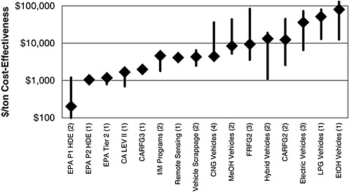
TABLE F-50 Adjusted Dollar-per-Ton Mobile Source Emission Control Costs: VOC-Equivalent Tons, 2000 dollars
used, variance of the expected values of costs and emission reductions, and other unreported bias. On the other hand, cost-effectiveness for some of the measures was estimated in only one study. Consequently, a range may not be available for published per-ton cost estimates. The lack of a range for some measures here does not necessarily indicate that less uncertainty is associated with the cost-effectiveness values of these measures.
Although precise quantitative conclusions cannot be drawn from Figure F-1, some general conclusions about the relative cost-effectiveness of various control measures can be drawn. On the basis of median cost-effectiveness values, in general, the most cost-effective measures are EPA’s Phase 1 and 2 HDE emission standards, EPA’s Tier 2 LDV emission standards, California’s LEV II program, California’s Phase 3 RFG, I&M programs, remote sensing programs, and old vehicle scrappage. These control measures have cost-effectiveness values of less than $10,000/ton. Separately, Beaton et al. (1995) showed that repairs or scrappage of old cars could be very cost-effective.
Figure F-1 shows that AFVs generally have high control costs and large variances in control costs. This implies technological uncertainties surrounding AFVs. Similar conclusions for AFVs were drawn by Krupnick and Walls (1992) and Hahn (1995). Besides having high control costs, AFVs may be subject to great market uncertainties because of potentially inferior attributes of some AFV types, fuel infrastructure inadequacy, and high initial costs to consumers.
Control of mobile source emissions focused on emissions of VOC, CO, and NOx until the early 1990s. The focus was then shifted to control emissions of VOC and NOx. In the late 1990s, the focus was shifted further to NOx emissions. In recent years, it has been found that PM emissions may cause more damage than do VOC and NOx emissions. Subsequently, attention began to be paid to the control of PM emissions. Because PM emission control is a relatively new phenomenon, most past cost-effectiveness studies did not analyze it. Consequently, data for PM control cost-effectiveness are scarce. Among the reviewed studies, only two estimated dollar-per-ton costs for PM emissions. The PM control costs from two studies are summarized in Table F-51. The table shows significant increases between PM control costs from an EPA study and the adjusted
TABLE F-51 PM Emission Control Costs ($/ton, 2000 dollars)
|
Control Program |
Original Estimate |
Adjusted Estimate |
Change (%) |
||||
|
Low |
High |
Median |
Low |
High |
Median |
||
|
96 Diesel stand., Schimek (2001) |
2,641 |
2,641 |
2,641 |
2,800 |
2,800 |
2,800 |
6 |
|
Bus Retrofit, Schimek (2001) |
7,256 |
26,999 |
17,127 |
7,600 |
28,100 |
17,900 |
5 |
|
EPA Phase 2 HDE, EPA (2000c) |
4,195 |
14,237 |
9,216 |
40,000 |
135,800 |
87,900 |
854 |
|
Hybrid bus, Schimek (2001) |
70,006 |
341,794 |
205,900 |
73,000 |
356,300 |
214,600 |
4 |
|
CNG bus, Schimek (2001) |
184,144 |
298,963 |
241,553 |
192,000 |
311,600 |
251,800 |
4 |
results in this study. This is caused by excluding PM emission reductions in PM air quality attainment areas in this study.
Table F-51 shows that the 1996 diesel PM emission standard and the bus retrofitting program could be cost-effective in reducing PM emissions. In general, cost estimates of PM emission control were not dealt with adequately in past studies. One problem is that modeling of PM emissions is much less accurate. If PM emissions had been treated adequately in past studies, some of the evaluated control measures, which help reduce PM emissions, might have had favorable cost-effectiveness results. Such measures include EPA’s light-duty Tier 2 program, CARB’s LEV II program, I&M programs, remote sensing programs, and AFVs.
PM damage values are much higher than those for VOC and NOx. For example, McCubbin and Delucchi (1999) estimated that PM damage value could be 7 to 8 times as great as NOx damage value. This implies that even with PM emission control costs as high as 7 to 8 times those of NOx, PM control measures could still be as effective as NOx control measures in reducing air pollution damage.
CONCLUSIONS
Calculating the cost-effectiveness of mobile source control measures involves dealing with both methodological and technical issues. Technical issues are related to values assumed for costs and emission reductions, whereas methodological issues are related to which costs are accounted for, how emission reductions are calculated, and which pollutants are included. To adequately (and correctly) estimate comparable cost-effectiveness, the following methodologies should be
consistently applied to mobile source cost-effectiveness calculations. For cost estimation, societal (as well as user) costs need to be considered, and costs should be estimated at the consumer rather than the manufacturer level. For emission reduction estimation, baseline emissions should be calculated by taking into account the control programs already implemented. Although emissions in nonattainment seasons and nonattainment areas are directly related to attainment of air quality standards, emissions in attainment seasons and attainment areas should not be treated as having zero value. For control measures that reduce emissions of multiple pollutants, emission reductions of all affected pollutants should be taken into account. To be consistent with cost estimates where discounting is applied, discounting should be applied to emissions as well.
The studies reviewed in this report show wide ranges in cost-effectiveness for control measures, attributable to both methodological and technical differences. Because of the different methodologies used in the studies, their cost-effectiveness estimates are not comparable. Limited methodological adjustments were made to the original estimates in this study to allow a consistent comparison of the study results.
Although precise quantitative conclusions cannot be drawn from the adjusted cost-effectiveness results, the results show general trends in the relative cost-effectiveness of various mobile source control measures. In general, among the mobile source control measures evaluated, the most cost-effective measures are EPA’s Phase 1 and 2 HDE emission standards, EPA’s Tier 2 vehicle emission standards, the California LEV II program, California Phase 3 RFG, I&M programs, remote sensing programs, and old vehicle scrappage. These control measures have cost-effectiveness values of less than $10,000/ton.
APPENDIX: SUMMARY OF STATIONARY SOURCE EMISSION CONTROL COST-EFFECTIVENESS
Regulatory agencies, such as EPA, CARB, and local air districts, estimate control cost-effectiveness for stationary source emission control measures as well as for mobile source control measures. One of the extensive studies covering stationary and mobile source control measures was completed by E. H. Pechan and Associates for EPA (EPA 1997a; EPA 1997b; E. H. Pechan and Associates 1997). Pechan
estimated about 150 control measures, including seven mobile source control measures, to reduce emissions of VOC, NOx, particulate matter with size less than 10 microns (PM10), and SOx. The results were used by EPA to determine ways of meeting EPA-proposed ozone and PM ambient concentration standards in different U.S. regions.
In estimating control costs, Pechan used a 7 percent real-term discount rate to discount both costs and emissions over time. All costs were estimated in 1990 dollars. In this study, the 1990 dollar-based costs were converted into 2000 dollar-based costs.
In simulating the air quality effects of adopting various control measures, EPA decided to take all control measures with control costs below $10,000/ton (1990 dollars). The threshold of $10,000/ton was used for all pollutants (VOC, NOx, PM10, and SOx). However, recent assessments show that PM10 emissions could cause much more significant health damage than emissions of VOC and NOx (via ozone). Thus, the control cost threshold for PM10 emission control should have been set at a much higher level.
Tables F-52 through F-55 present dollar-per-ton control costs for stationary VOC, NOx, PM10, and SOx emissions, respectively. Pechan’s study indicated that each stationary source control measure reduced emissions of one pollutant only. Single-pollutant reduction measures are applicable to stationary source emission control, since stationary control measures can be designed to reduce emissions of one pollutant. Thus, estimation of stationary source control cost-effectiveness did not face the issue of multiple-pollutant emission reductions, as mobile source control measures usually do.
Table F-52 presents dollar-per-ton costs for VOC control in terms of tons of VOC emissions reduced; Table F-53 presents dollar-per-ton costs for NOx control in terms of tons of NOx emissions reduced; Table F-54 presents dollar-per-ton costs for PM10 control in terms of tons of PM10 emission reduced; and Table F-55 presents dollar-per-ton costs for SOx emissions in terms of tons of SOx emissions reduced. That is, each individual table presents the costs to reduce a ton of the pollutant being evaluated. On the other hand, the results presented in the section summarizing the original and adjusted estimates of mobile source cost-effectiveness values are for a ton of VOC-equivalent emissions. Readers cannot directly compare results in
TABLE F-52 Stationary Source VOC Control Costs: VOC Tons ($/ton, 2000 dollars)
TABLE F-53 Stationary Source NOxControl Costs: NOxTons ($/ton, 2000 dollars)
|
Control Measure |
Low |
High |
Average |
|
Low-emission combustion for NG-fired IC engines |
0 |
15,500 |
200 |
|
Low-NOx burners for NG-fired ICI boilers |
0 |
1,700 |
400 |
|
Low-NOx burners for iron and steel mills |
400 |
400 |
400 |
|
Low-NOx burners for NG gas turbines |
300 |
6,700 |
600 |
|
Mid-kiln firing for wet cement manufacture |
600 |
600 |
600 |
|
Ignition timing retard for oil-fired IC engines |
200 |
700 |
600 |
|
Low-NOx burners for oil process heater |
600 |
600 |
600 |
|
Ignition timing retard for NG, diesel, LPG-fired IC engines |
600 |
1,000 |
700 |
|
Mid-kiln firing for dry cement manufacture |
700 |
700 |
700 |
|
Mid-kiln firing for lime kilns |
700 |
700 |
700 |
|
O2 trim and water injection for NG reformers in ammonia plants |
900 |
900 |
900 |
|
Low-NOx burners for LPG process heater |
900 |
900 |
900 |
|
O2 trim water injection for NG space heater |
900 |
1,000 |
900 |
|
Low-NOx burners for industrial NG combustion |
800 |
1,100 |
900 |
|
Low-NOx burners for oil reformers in ammonia plants |
1,200 |
1,200 |
1,200 |
|
Low-NOx burners for industrial oil combustion |
100 |
2,500 |
1,200 |
|
SNCR for coke-fired ICI boilers |
400 |
3,300 |
1,400 |
|
O2 trim water injection for NG-fired ICI boilers |
0 |
14,900 |
1,400 |
|
Urea-based SNCR for dry cement manufacture |
1,500 |
1,500 |
1,500 |
|
Water injection for oil-fired gas turbines |
1,500 |
1,500 |
1,500 |
|
SNCR for lime kilns |
1,500 |
1,500 |
1,500 |
|
SCR for coal-fired utility boilers |
1,100 |
3,200 |
1,500 |
|
Low-NOx burners for oil-fired ICI boilers |
100 |
44,000 |
1,600 |
|
Low-NOx burner flue gas recirculation for iron and steel mills |
1,600 |
1,700 |
1,600 |
|
Low-NOx burners for industrial coal combustion |
800 |
2,600 |
1,600 |
|
Low-NOx burners for diesel process heater |
400 |
3,700 |
1,700 |
|
Low-NOx burners for NG process heater |
0 |
17,000 |
1,900 |
|
Low-NOx burners for LPG-fired ICI boilers |
0 |
8,900 |
2,400 |
|
SCR for NG, diesel, LPG-fired IC engines |
1,400 |
2,900 |
2,500 |
|
SCR for oil-fired IC engines |
1,400 |
6,000 |
2,600 |
|
SNCR for coal-fired ICI boilers |
400 |
14,500 |
3,100 |
|
SCR for container glass manufacture |
2,100 |
6,400 |
3,200 |
|
SNCR for commercial/institutional incinerators |
3,400 |
3,400 |
3,400 |
|
SNCR for industrial and medical incinerators |
2,900 |
15,200 |
3,400 |
|
SNCR for municipal waste combustion |
3,400 |
3,400 |
3,400 |
|
NG reburn for coal-fired ICI boilers |
3,600 |
3,600 |
3,600 |
|
Low-NOx burners for coke-fired ICI boilers |
2,900 |
4,800 |
3,800 |
|
Low-NOx burners flue gas recirculation for oil-fired ICI boilers |
1,300 |
6,100 |
3,900 |
|
Low-NOx burners for coal-fired ICI boilers |
400 |
57,600 |
4,000 |
|
Low-NOx burners for diesel-fired ICI boilers |
300 |
61,100 |
5,200 |
|
SCR for wet cement manufacture |
5,900 |
5,900 |
5,900 |
|
SCR for oil reformers in ammonia plants |
6,200 |
6,200 |
6,200 |
|
SCR for NG reformers in ammonia plants |
0 |
27,500 |
9,500 |
|
Low-NOx burners flue gas recirculation for LPG-fired ICI boilers |
8,700 |
11,300 |
10,000 |
Tables F-53 through F-55 with the results in that section, since the tonnage in each of the tables here is not the same as in that section, except for VOC emission controls in Table F-52.
Of the 40 stationary VOC control measures in Table F-52, 24 have control costs below $10,000 (average values in the table) per ton of
TABLE F-54 Stationary Source PM10Control Costs: PM10Tons ($/ton, 2000 dollars)
TABLE F-55 Stationary Source SOxControl Costs: SOxTons ($/ton, 2000 dollars)
VOC emissions reduced; 14 have control costs between $10,000 and $20,000; and 2 have control costs between $25,000 and $27,000. Note that a negative control cost number in the table means that the monetary benefit of a given control measure exceeds the cost of the control measure. On the other hand, Table F-50 shows that except for AFVs, mobile source control measures have control costs below $10,000/ton. Mobile source control measures appear to be competitive with stationary VOC control measures.
Table F-53 presents 76 stationary NOx control measures. Among them, 44 have control costs below $10,000 (average values in the table) per ton of NOx emissions reduced; 10 have control costs between $10,000 and $20,000 per NOx ton; and the remaining 22 have control costs above $20,000 per NOx ton. In comparing these results with those in Table F-50, the results under the 1:0:1 weighting factor set in Table F-50 should be used, since this set treats 1 NOx ton the same as 1 VOC ton. Table F-50 shows that 8 of the 16 mobile source control measures have emission control costs below $10,000; 2 have control costs between $10,000 and $20,000; and the remaining 6 have control costs above $20,000. Mobile and stationary control measures are competitive with each other in terms of NOx control costs. However, both mobile and stationary control measures have higher NOx control costs than VOC control costs.
Table F-54 shows costs for 22 stationary PM10 control measures. Among them, 12 have PM10 control costs below $10,000 per PM10 ton; 4 have control costs between $10,000 and $20,000; and the remaining 6 have control costs above $20,000 (with 2 having control costs above $200,000 per PM10 ton). On the other hand, among the five mobile PM10 control measures included in Table F-51, only two have control costs below $20,000. The other three have control costs between $88,000 and $250,000 per PM10 ton. Though it appears that control of mobile source PM10 emissions is more costly than control of stationary PM10 emissions, one needs to be cautious with such an interpretation. Of the PM10 emissions reduced, stationary control measures may reduce emissions of large-size PM (e.g., PM2.5 to PM10), while mobile source control measures may reduce fine PM (e.g., PM2.5 and smaller). Assessments have shown that fine PM is more damaging to health than is large-size PM. Mobile source fine PM emission control could
be as cost-effective as or more cost-effective than stationary fine PM emission control. In addition, Table F-54 (and Tables F-52 and F-53) shows that many of the stationary control measures are for large stationary facilities, which are usually located outside of populated areas. On the other hand, motor vehicles are concentrated in populated areas, and large populations are exposed to their emissions. The geographic locations of mobile and stationary source emissions imply that mobile source emissions may cause more damage to health than do stationary source emissions. This could justify implementation of some mobile source control measures, which could have higher control costs than stationary source control measures.
Table F-55 presents control costs for stationary SOx control measures. The table shows that scrubbers can be expensive in reducing SOx emissions, considering the value of $4,800/ton of SOx emissions that was used by EPA in evaluating its Tier 2 vehicle standards (see the section on review of past studies).
Table F-56 presents Pechan’s results for seven mobile source control measures. For mobile source control measures reducing emissions of multiple pollutants, Pechan combined emissions of VOC, NOx, and PM10 according to their contributions to ambient PM10 concentrations. This requires detailed air quality modeling, and it is conceivable that each control measure could have different weighting factors.
TABLE F-56 Mobile Source Emission Control Costs ($/ton, 2000 dollars)
|
Control Measure |
Low |
High |
Average |
|
Enhanced I&M programs |
500 |
1,000 |
800 |
|
FRFG2 for off-road vehicles |
200 |
32,600 |
5,300 |
|
FRFG2 for on-road vehicles |
4,500 |
30,500 |
7,700 |
|
Off-road HDDV retrofit program |
10,000 |
16,800 |
11,400 |
|
On-road HDDV retrofit program |
30,700 |
30,900 |
30,700 |
|
Fleet ILEV |
7,900 |
91,300 |
27,000 |
|
Tier 2 standards for LDGT |
6,800 |
64,400 |
42,900 |
|
Notes: These control measures reduce emissions of VOC, NOx, and PM10. They were combined by Pechan according to their contributions to ambient PM concentrations. Note also earlier discussion in the text regarding comparability of results in this table with those in Table F-50. |
|||
Considering the mechanism of PM formation in the atmosphere, it is likely that Pechan’s implicit weighting factors could be between the base case and the NOx-important weighting factor sets established in this study (Table F-12). Thus, the results in Table F-56 are compared with the results under those two weighting factor sets in Table F-50.
Tables F-50 and F-56 show that I&M programs and RFG could be cost-effective. Table F-50 does not include heavy-duty diesel vehicle (HDDV) retrofits, so those results in Table F-56 cannot be compared. The fleet ILEV (inherently low-emission vehicle) program in Table F-56 was meant to be CNG vehicles. Table F-50 shows much lower control costs for CNG vehicles ($4,550/ton under the base case weighting factors and $2,300/ton under the NOx-important weighting factors) than does Table F-56 ($27,000/ton). The Tier 2 standards in Table F-56 were the standards specified in the CAAA, which were less stringent than EPA’s final Tier 2 standards. However, even with less stringent Tier 2 standards, Pechan’s cost estimates were much higher than EPA’s cost estimates.
The above sections show the cost-effectiveness of mobile and stationary source control measures. The cost-effectiveness result of a given control measure does not indicate by how much the particular measure can reduce emissions, which is beyond the scope of this study. To provide some hints about the potential magnitude of emission reductions achievable by the control measures evaluated in this study, Table F-57 presents emission inventory data for 1999 in the United States. The table indicates major emission sources for a given pollutant. One can examine the control measures evaluated in this study together with the emission inventory data in the table to determine whether a given control measure targets major emission sources. If so, the control measure should be able to provide a large quantity of emission reductions.
ACKNOWLEDGMENTS
This study was funded by the Transportation Research Board of the National Research Council. The author is grateful to directions and guidelines from the Committee for the Evaluation of the Congestion Mitigation and Air Quality Improvement Program of the Transportation Research Board. In particular, the author thanks Nancy Humphrey, the project manager, and Alan Krupnick and Ken Small,
TABLE F-57 U.S. Annual Emissions from Different Sources (thousands of tons in 1999) (EPA 2001)
two committee members, for their helpful comments and suggestions. The author is solely responsible for the contents of this report.
REFERENCES
Abbreviations
CAIMRC California Inspection and Maintenance Review Committee
CARB California Air Resources Board
EIA Energy Information Administration
EPA U.S. Environmental Protection Agency
NPC National Petroleum Council
NRC National Research Council
Alberini, A., D. Edelstein, W. Harrington, and V. McConnell. 1994. Reducing Emissions from Old Cars: The Economics of the Delaware Vehicle Retirement Program. Discussion Paper 94-27. Resources for the Future, Washington, D.C., April.
Ando, A., V. McConnell, and W. Harrington. 2000. Costs, Emissions Reductions, and Vehicle Repair: Evidence from Arizona. Journal of the Air and Waste Management Association, Vol. 50, No. 4, April, pp. 509–521.
Beaton, S. P., G. A. Bishop, Y. Zhang, L. A. Ashbaugh, D. R. Lawson, and D. H. Stedman. 1995. On-Road Vehicle Emissions: Regulations, Costs, and Benefits. Science, Vol. 268, May 19, pp. 991–993.
CAIMRC. 2000. Smog Check II Evaluation. Sacramento, Calif., June 19.
CARB. 1990. Proposed Regulations for Low-Emission Vehicles and Clean Fuels, Staff Report. Sacramento, Calif., Aug. 13.
CARB. 1991. Proposed Regulations for California Phase 2 Reformulated Gasoline, Technical Support Document. Sacramento, Calif., Oct. 4.
CARB. 1993. Mobile Source Emission Reduction Credits, Guidelines for the Generation and Use of Mobile Source Emission Reduction Credits. Stationary Source Division and Mobile Source Division, Sacramento, Calif., Feb. 19.
CARB. 1994. Staff Report: 1994 Low-Emission Vehicle and Zero-Emission Vehicle Program Review. Mobile Source Division, El Monte, Calif., April.
CARB. 1996. Facts About Cleaner-Burning Gasoline. Stationary Source Division, Sacramento, Calif., March.
CARB. 1998. Staff Report: Initial Statement of Reasons, Proposed Amendments to California Exhaust and Evaporative Emission Standards and Test Procedures for Passenger Cars, Light-Duty Trucks and Medium-Duty Vehicles “LEV II.” Mobile Source Control Division, El Monte, Calif., Sept. 18.
CARB. 1999. Proposed California Phase 3 Reformulated Gasoline Regulations: Proposed Amendments to the California Reformulated Gasoline Regulations, Including a December 31, 2002 Prohibition of Using MTBE in Gasoline, Adoption of Phase 3 Gasoline Standards, a Phase 3 Predictive Model, and Other Changes, Staff Report: Initial Statement of Reasons. Sacramento, Calif., Oct. 22.
CARB. 2000. Staff Report: Initial Statement of Reasons, Proposed Amendments to the California Zero Emission Vehicle Program Regulations. Mobile Source Division, Sacramento, Calif., Dec. 8.
Dill, J. 2000. Vehicle Scrappage Programs. Presented at the NRC CMAQ Review Committee Meeting, Berkeley, Calif., Oct. 13.
Dill, J. 2001. Design and Administration of Accelerated Vehicle Retirement Programs in North America and Abroad. In Transportation Research Record: Journal of the Transportation Research Board, No. 1750, TRB, National Research Council, Washington, D.C., pp. 32–39.
E. H. Pechan and Associates. 1997. Additional Control Measure Evaluation for the Integrated Implementation of the Ozone and Particulate Matter National Ambient Air Quality Standards, and Regional Haze Program.
Prepared for Office of Air Quality Planning and Standards, U.S. Environmental Protection Agency, Research Triangle Park, N.C., July 17.
EIA. 2000. Estimated Number of Alternative-Fueled Vehicles in Use in the United States. www.eia.doe.gov. Feb. 29.
EPA. 1994. Regulation of Fuels and Fuel Additives; Standards for Reformulated and Conventional Gasoline; Final Rule. Federal Register, Feb. 16.
EPA. 1997a. Regulatory Impact Analyses for the Particulate Matter and Ozone National Ambient Air Quality Standards and Proposed Regional Haze Rule. EPAOAQ 0041187. Innovative Strategies and Economics Group, Office of Air Quality Planning and Standards, Research Triangle Park, N.C., July 16.
EPA. 1997b. Regulatory Impact Analyses for the Particulate Matter and Ozone National Ambient Air Quality Standards and Proposed Regional Haze Rule, Appendix A: Emissions and Air Quality. EPAOAQ 0041605. Innovative Strategies and Economics Group, Office of Air Quality Planning and Standards, Research Triangle Park, N.C., July 16.
EPA. 1999. Regulatory Impact Analysis—Control of Air Pollution from New Motor Vehicles: Tier 2 Motor Vehicle Emissions Standards and Gasoline Sulfur Control Requirements. EPA420-R-99-023. Washington, D.C., Dec.
EPA. 2000a. Control of Air Pollution from New Motor Vehicles: Tier 2 Motor Vehicle Emissions Standards and Gasoline Sulfur Control Requirements; Final Rule. Federal Register, Feb. 10.
EPA. 2000b. Control of Emissions of Air Pollution from 2004 and Later Model-Year Heavy-Duty Highway Engines and Vehicles; Revision of Light-Duty On-Board Diagnostics; Notice of Final Rulemaking. Washington, D.C., July.
EPA. 2000c. Control of Air Pollution from New Motor Vehicles: Heavy-Duty Engine and Vehicle Standards; Highway Diesel Fuel Sulfur Control Requirements; Final Rule. Federal Register, Dec. 21.
EPA. 2001. National Air Quality and Emissions Trends Report, 1999. EPA454-R-01-004. Office of Air Quality Planning and Standards, Research Triangle Park, N.C., March.
Greene, D. L., and P. N. Leiby. 1993. The Social Costs to the U.S. of Monopolization of the World Oil Market. Report ORNL-6744. Oak Ridge National Laboratory, Oak Ridge, Tenn., March.
Hadder, G. R. 1995. A Comparison of Estimates of Cost-Effectiveness of Alternative Fuels and Vehicles for Reducing Emissions. ORNL/TM-13110. Center for Transportation Analysis, Oak Ridge National Laboratory, Oak Ridge, Tenn., Nov.
Hahn, R. W. 1995. Choosing Among Fuels and Technologies for Cleaning Up the Air. Journal of Policy Analysis and Management, Vol. 14, No. 4, pp. 532–554.
Harrington, W., and V. D. McConnell. 1993. Cost-Effectiveness of Remote Sensing of Vehicle Emissions. Discussion Paper QE93-24. Resources for the Future, Washington, D.C., Sept.
Harrington, W., V. D. McConnell, and A. Ando. 1999. The Enhanced I&M Program in Arizona: Costs, Effectiveness, and a Comparison with Pre-
Regulatory Estimates. Discussion Paper 99-37. Resources for the Future, Washington, D.C., June.
Harrington, W., V. McConnell, and A. Ando. 2000. Are Vehicle Emission Inspection Programs Living Up to Expectations? Transportation Research D, Vol. 5, pp. 153–172.
Krupnick, A. J., and M. A. Walls. 1992. The Cost-Effectiveness of Methanol for Reducing Motor Vehicle Emissions and Urban Ozone. Journal of Policy Analysis and Management, Vol. 11, No. 3, pp. 373–396.
Lareau, T. J. 1994. Improving Cost-Effectiveness Estimation: A Reassessment of Control Options to Reduce Ozone Precursor Emissions. American Petroleum Institute, Washington, D.C., Aug.
Lave, L. B., and H. L. Maclean. 2001. Are Hybrid Vehicles Worth It? IEEE Spectrum, March, pp. 47–50.
McCubbin, D. R., and M. A. Delucchi. 1999. The Health Costs of Motor-Vehicle-Related Air Pollution. Journal of Transport Economics and Policy, Vol. 33, Part 3, pp. 253–286.
NPC. 1993. U.S. Petroleum Refining: Meeting Requirements for Cleaner Fuels and Refineries, Volume V—Refining Capability Appendix. Washington, D.C., Aug.
NRC. 2000. Ozone-Forming Potential of Reformulated Gasoline. National Academy Press, Washington, D.C.
Schimek, P. 2001. Reducing Emissions from Transit Buses. Regional Science and Urban Economics, Vol. 31, pp. 433–451.
Sierra Research, Inc. 1991. Cost-Effectiveness Analysis of CARB’s Proposed Phase 2 Gasoline Regulations. Prepared for Western States Petroleum Association, Sacramento, Calif., Nov. 18.
Sierra Research, Inc. 1994. The Cost-Effectiveness of Further Regulating Mobile Source Emissions. Prepared for American Automobile Manufactures Association, Sacramento, Calif., Feb. 28.
Sierra Research, Inc. 1998. Evaluation of VOC and NOx Control Measures. Prepared for Western States Petroleum Association, Sacramento, Calif., April.
Wang, Q., C. Kling, and D. Sperling. 1993a. Light-Duty Vehicle Exhaust Emission Control Cost Estimates Using a Part-Pricing Approach. Journal of the Air and Waste Management Association, Vol. 43, pp. 1461–1471.
Wang, Q., D. Sperling, and J. Olmstead. 1993b. Emission Impacts, Life-Cycle Cost Changes, and Emission Control Cost-Effectiveness of Methanol-, Ethanol-, Liquefied Petroleum Gas-, Compressed Natural Gas-, and Electricity-Powered Vehicles. Research Report UCD-ITS-RR-93-7. Institute of Transportation Studies, University of California at Davis, Davis, May 9.
Wang, M. Q., D. J. Santini, and S. A. Warinner. 1994. Methods of Valuing Air Pollution and Estimated Monetary Values of Air Pollutants in Various U.S. Regions. Report ANL/ESD-26. Argonne National Laboratory, Argonne, Ill., Dec.
Wang, M. Q. 1997. Mobile Source Emission Control Cost-Effectiveness: Issues, Uncertainties, and Results. Transportation Research D, Vol. 2, pp. 43–56.


