
5
Earthquake Physics and Fault-System Science
Earthquake research focuses on two primary problems. Basic earthquake science seeks to understand how earthquake complexity arises from the brittle response of the lithosphere to forces generated within the Earth’s interior. Applied earthquake science seeks to predict seismic hazards by forecasting earthquakes and their site-specific effects. Research on the first problem began with attempts to place earthquake occurrence in a global framework, and it contributed to the discovery of plate tectonics; research on the second was driven by the needs of earthquake engineering, and it led to the development of seismic hazard analysis. The historical separation between these two problems, reviewed in Chapter 2, has been narrowed by an increasing emphasis on dynamical explanations of earthquake phenomena. In this context, the term dynamics implies a consideration of the forces (stresses) within the Earth that act to cause fault ruptures and ground displacements during earthquakes. The stress fields responsible for deep-seated earthquake sources cannot be measured directly, but they can be inferred from models of earthquake systems that obey the laws of physics and conform to the relationships between stress and deformation (rheology) observed in the laboratory.
This chapter describes how this physics-based approach has transformed the field into an interdisciplinary, system-level science—one in which dynamical system models become the means to explain and integrate the discipline-based observations discussed in Chapter 4. The chapter begins with an essay on the central problems of dynamics and prediction, which is followed by five sections on areas of intense interdisciplinary research: fault systems, fault-zone processes, rupture dynam-
ics, wave propagation, and seismic hazard analysis. Each of the latter summarizes the current understanding and articulates major goals and key questions for future research.
5.1 EARTHQUAKE DYNAMICS
For present purposes, the term “dynamical system” can be understood to mean any set of coupled objects that obeys Newton’s laws of motion—rocks or tectonic plates, for example (1). If one can specify the positions and velocities of each of these objects at any given time and also know exactly what forces act on them, then the state of the system can be determined at a future time, at least in principle. With the advent of large computers, the numerical simulation of system behavior has become an effective method for predicting the behavior of many natural systems, especially in the Earth’s fluid envelopes (e.g., weather, ocean currents, and long-term climate change) (2). However, many difficulties face the application of dynamical systems theory to the analysis of earthquake behavior in the solid Earth. Forces must be represented as tensor-valued stresses (3), and the response of rocks to imposed stresses can be highly nonlinear. The dynamics of the continental lithosphere involves not only the sudden fault slips that cause earthquakes, but also the folding of sedimentary layers near the surface and the ductile motions of the hotter rocks in the lower crust and upper mantle. Moreover, because earthquake source regions are inaccessible and opaque, the state of the lithosphere at seismogenic depths simply cannot be observed by any direct means, despite the conceptual and technological breakthroughs described in Chapter 4.
From a geologic perspective, it is entirely plausible that earthquake behavior should be contingent on a myriad of mechanical details, most unobservable, that might arise in different tectonic environments. Yet earthquakes around the world share the common scaling relations, such as those noted by Gutenberg and Richter (Equation 2.5) and Omori (Equation 2.8). The intriguing similarities among the diverse regimes of active faulting make earthquake science an interesting testing ground for concepts emerging from the physics of complex dynamical systems. One consequence of recent interactions between these fields is that theoretical physicists have adopted a family of idealized models of earthquake faults as one of their favorite paradigms for a broad class of nonequilibrium phenomena (4). At the same time, earthquake scientists have become aware that earthquake faults may be intrinsically chaotic, geometrically fractal, and perhaps even self-organizing in some sense. As a result, an entirely new subdiscipline has emerged that is focused around the development and analysis of large-scale numerical simulations of deformation
dynamics. Combined with insightful physical reasoning and intriguing new laboratory and field data, these investigations promise a better understanding of seismic complexity and predictability.
Complexity and the Search for Universality
Earthquakes are clearly complex in both the commonsense and the technical meanings of the word. At the largest scales, complexity is manifested by features such as the aperiodic intervals between ruptures, the power-law distribution of event frequency across a wide range of magnitudes, the variable patterns of slip for earthquakes occurring at different times on a single fault, and the richness of aftershock sequences. Individual events are also complex in the disordered propagation of their rupture fronts and the heterogeneous distributions of residual stress that they leave in their wake. At the smallest scales, earthquake initiation appears to be complex, with a slowly evolving nucleation zone preceding a rapid dynamic breakout that sometimes cascades into a big rupture. Among the many open issues in this field are the questions of whether these different kinds of complexity might be related to one another and, if so, how.
The most ambitious and optimistic reason for considering the ideas of dynamical systems theory is the hope that one might discover universal features of earthquake-like phenomena. Such features would, of course, be extremely interesting from a fundamental scientific point of view. They might also have great practical value, for example, as a basis for interpreting seismic records or for making long-term hazard assessments. Two thought-provoking, complementary concepts that look as if they might bring some element of universality to earthquake science are fractality and self-organized criticality. The first describes the geometry of fault systems; the second is an intrinsically dynamic hypothesis that pertains to the complex motions of these systems. Although each has provoked its own point of view among earthquake scientists—that seismic complexity is, on the one hand, primarily geometric in origin or, on the other hand, primarily dynamic—it seems likely that both concepts contain some elements of the truth and that neither is a complete description of the behavior of the Earth.
There is substantial evidence that fault geometry is fractal, at least in some cases and over some ranges of length scales. Fractality is a special kind of geometric complexity that is characterized by scale invariance (5). That is, images of the same system made with different magnifications are visually similar to one another; there is no intrinsic length scale such as a correlation length or a feature of recognizable size that would enable an observer to determine the magnification simply by looking at the image.
One result of such a property in the case of fault zones is that there would be a broad, power-law distribution of the lengths of the constituent fault segments (6). If, in the simplest conceivable scenario, the seismic moment of the characteristic earthquake on each segment were proportional to its length, and each segment slipped at random, then the moment distribution would also be a power law. This picture is too simplistic to be a plausible explanation of the Gutenberg-Richter relation, but it may contain some element of the truth.
Self-organized criticality refers to the conjecture that a large class of physical systems, when driven persistently away from mechanical equilibrium, will operate naturally near some threshold of instability, and will therefore exhibit something like thermodynamic critical fluctuations (7). Earthquake faults, or arrays of coupled faults, seem to be natural candidates for this kind of behavior; such systems are constantly being driven by tectonic forces toward slipping thresholds (8). If the thermodynamic analogy were valid, then the fluctuations—the slipping events—would be self-similar and scale invariant, and their sizes would obey power-law distributions. More important, systems with this self-organizing property would always be at or near their critical points. Critical behavior, with strong sensitivity to small perturbations and intrinsic unpredictability, would be a universal characteristic of such systems.
Elementary Models of Earthquake Dynamics
The ideas of fractality and dynamic self-organization have inspired a wide range of theoretical models of seismic systems. These models are almost invariably numerical: that is, they are studied primarily by means of large-scale computation. One class is cellular automata in which highly simplified rules for the behavior of large numbers of coupled components attempt to capture the essential features of complex seismic systems (9). Almost all cellular automata are related in some ways to the original one-dimensional slider-block model of Burridge and Knopoff (10), illustrated in Figure 5.1. Perhaps the most important result to emerge from such studies so far is the discovery that some of the simplest of these models, even the completely uniform Burridge-Knopoff model with a plausible, velocity-weakening dynamic friction law, are deterministically chaotic (11).
A chaotic system, by definition, is one in which the accuracy needed to determine its motion over some interval of time grows rapidly, in fact exponentially, with the length of the interval. Two identical systems that are set in motion with almost but not quite the same initial conditions may move in nearly the same way for a while. If these systems are chaotic, however, their motions eventually will differ from each other and, after a
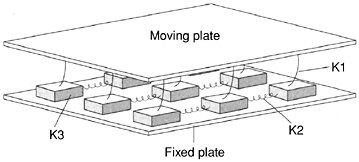
FIGURE 5.1 Two-dimensional version of the Burridge-Knopoff spring-slider model. Leaf springs (K1) connect a moving plate to an array of smaller sliding blocks. These blocks are in turn connected to their nearest neighbors via coil springs (K2, K3). Sliding blocks also have a frictional contact with a fixed plate. Simulated earthquakes from models of this type display a wide variety of complexity. SOURCE: P. Bak, How Nature Works: The Science of Self-Organized Criticality, Springer-Verlag, New York, 226 pp., 1996. Copyright permission granted by Springer-Verlag.
sufficiently long time, will appear to be entirely uncorrelated. The correlation time depends sensitively on the difference in the initial conditions. In the context of predictability, this means that any uncertainty in one’s knowledge of the present state of a deterministically chaotic system produces a theoretical limit on how far into the future one can determine its behavior reliably, a topic explored further below.
One theoretical issue that has attracted a lot of attention has come to be known as the question of smooth versus heterogeneous fault models. This issue arose initially as a result of the unexpected success of the uniform Burridge-Knopoff slider-block models in producing very rough but interesting caricatures of complex earthquake-like behavior, which fueled speculation that some of the slip complexity of natural earthquakes might be generated by the nonlinear dynamics of stressing and rupture on essentially smooth and uniform faults. The more conventional and perhaps obvious assumption is that the heterogeneity of fault zones—their geometric disorder and strong variations of lithological properties—plays the dominant role. It appears that earthquake faults, when modeled in any detail, have relevant length and time scales that invalidate simple scaling assumptions. For example, the tectonic loading speed (meters per century) combined with known friction thresholds and elastic moduli of rocks suggests natural characteristic intervals (hundreds of years) between large slipping events. Models that incorporate these features produce event distributions in which the large events fail to be self-similar (12).
Another example is the thickness of the seismogenic layer, which is less than the rupture scale for larger earthquakes. It, too, seems likely to produce scaling violations both in dynamic behavior and in the geometry of fault systems (see Section 5.2).
The existence of relevant length and time scales does not, per se, invalidate dynamical scaling theories; it may merely limit their ranges of validity. In some smooth-fault models, for example, it appears that the small, localized seismic events are self-similar over broad ranges of sizes; however, the large, delocalized events look quite different and are substantially more frequent than would be predicted by extrapolating the scaling distribution for the small events (13), as in the “characteristic earthquake” model discussed in Section 2.6. The picture may change appreciably if one considers large arrays of coupled faults and, especially, if one includes the mechanism for creation of new faults as a part of the dynamical system. It is possible that this global system, in some as yet poorly understood average sense, may come closer to a pure form of self-organized criticality.
Chaos and Predictability
The theoretical issue of earthquake predictability (as distinct from the practical issue of how to predict specific earthquakes) remains a central, unresolved issue. The wide range of event sizes described by the Gutenberg-Richter law, the obvious irregularities in intervals between large events, the fact that chaotic behavior occurs commonly in very simple earthquake-like models, and many other clues, all argue in favor of chaos and thus for an intrinsic limit to predictability. The interesting question is what bearing this theoretical limit might have on the kinds of earthquake prediction that are discussed elsewhere in this report. If one could measure all the stresses and strains in the neighborhood of a fault with great accuracy, and if one knew with confidence the physical laws that govern the motion of such systems, then the intrinsic time limit for predictability might be some small multiple of the average interval between characteristic large events on the fault. Most of the seismic energy is released in the large events; thus, it seems reasonable to suppose that the system suffers most of its memory loss during those events as well. If this supposition were correct, earthquake prediction on a time scale of months or years—intermediate-term prediction of the sort described in Section 2.6—would, in principle, be possible.
The difficulty, of course, is that one cannot measure the state of a fault and its surroundings with great accuracy, and one still knows very little about the underlying physical laws. If these gaps in knowledge could be filled, then predicting earthquakes a few years into the future might be no
more difficult than predicting the weather a few hours in advance. However, the geological information needed for earthquake prediction is far more complex than the atmospheric information required for weather prediction, and almost all of it is hidden far beneath the surface of the Earth. Thus, the practical limit for predictability may have little to do with the theory of deterministic chaos, but may be fixed simply by the sheer mass of information that is unavailable.
Progress Toward Realism
Two general goals of research in this field are to understand (1) how rheological properties of the fault-zone material interact with rupture propagation and fault-zone heterogeneity to control earthquake history and event complexity, and (2) to what extent scientists can use this knowledge to predict, if not individual earthquakes, then at least the probabilities of seismic hazards and the engineering consequences of likely seismic events. Finding the answers is an ambitious and difficult task, but there are reasons for optimism. The speeds and capacities of computers continue to grow exponentially; they are now at a point where numerical simulations can be carried out on scales that were hardly imagined just a decade ago. At the same time, the sensitivity and precision of observational techniques are providing new ways to test those simulations.
There exists, at present, a substantial theoretical and computational effort in the United States and elsewhere devoted to developing increasingly realistic models of earthquake faults. Given a situation in which such a wide variety of physical ingredients of a problem remain unconstrained by experiment or direct observation, numerical experiments to show which of these ingredients are relevant to the phenomena may be crucial. Consider, for example, the assumptions about friction laws that are at the core of every fault model. For slow slip, the rate- and state-dependent law discussed in Section 4.4 may be reliable, at least in a qualitative sense. On the other hand, for fast slip of the kind that occurs in large events, there is little direct information. It seems likely that dynamic friction in those cases is determined by the behavior of internal degrees of freedom such as fault gouge, pore fluids, and the like. Laboratory experiments on multicomponent lubricated interfaces may provide some insight, but the solution to this problem may have to rely on comparisons between real and simulated earthquakes. There are suggestions that a friction law with enhanced velocity-weakening behavior (i.e., stronger than the logarithmic weakening in the rate and state laws) is needed to produce slip complexity and perhaps also to produce propagating slip pulses in big events (14). This conjecture needs to be tested.
Friction is not the only constitutive property that may be relevant. The laws governing deformation and fracture may play important roles, especially if the latter processes are effective in arresting large events and/or creating new fault surfaces. Other uncertainties in this category include the geometric structure of faults, the ways in which constitutive properties vary as functions of depth or position along a fault, the statistical distribution of heterogeneities on fault surfaces, and the parameters that govern the interactions between neighboring faults during seismic events.
An equally serious issue is whether small-scale physical phenomena are relevant to large-scale behavior. A truly complete description of an earthquake would involve length and time scales ranging from the microscopic ones at which the dynamics of fracture and friction are determined to the hundreds of kilometers over which large events occur. Numerical simulations, especially three-dimensional ones, would be entirely infeasible if they were required to resolve such a huge range of scales. There are, however, examples in other scientific areas where this is precisely what occurs. In dendritic solidification, for example, it is known that a length scale associated with surface tension—a length usually on the order of ångströms—controls the shapes and speeds of macroscopic pattern formation (15). Any direct numerical simulation that fails to resolve this microscopic length scale produces qualitatively incorrect results. There are indications that similar effects occur in some hydrodynamic problems, perhaps even in turbulence (16).
At present, it is not known whether any such sensitivities occur in earthquake problems, but there are possibilities. For example, it remains an open question whether simulations of earthquakes must resolve the details of the initial fracture and/or the nucleation process. It is possible that many features of this small-scale behavior are imprinted in important ways on the subsequent large-scale events, but it is also possible that only one or two parameters pertaining to nucleation—perhaps the location and initial stress drop (plus the surrounding stress and strain fields, of course)—have to be specified in order to predict accurately what happens next. Similarly, if the solidification analogy is a guide, then the small-scale, high-frequency behavior of the constitutive laws might be relevant to pulse propagation, interactions between rupture fronts and heterogeneities, and mechanisms of rupture arrest.
In order to study large systems on finite computers, investigators frequently study two-dimensional models, often accounting for deformations in the crustal plane perpendicular to the fault (in models of transverse faults) and omitting or drastically oversimplifying variations in the fault plane (i.e., motions that are functions of depth beneath the surface). How relevant is the third dimension? Some investigators have argued
that it must be crucial because, without a coupling between the top and bottom of the fault, there is no restoring force to limit indefinitely large slip or, equivalently, to couple kinetic energy of slip back into stored elastic energy. It is hard to see how the dynamics of large events, especially rupture arrest and pulse propagation, can be studied sensibly without full three-dimensional analyses.
The issues of how to make progress toward realism are theoretical as well as computational. There is an emerging realization among theorists working on earthquake dynamics, and in solid mechanics more generally, that the problems with which they are dealing are far more difficult mathematically than they had originally supposed. One of the reasons that small-scale features can control large-scale behavior, as mentioned above, is that these features enter the mathematical statement of the problem as singular perturbations. For example, the surface tension in the solidification problem and the viscosity in certain shock-front problems enter the equations of motion as coefficients of the highest derivative of the dependent variable. As such, they completely change the answer to questions as basic as whether or not physically acceptable solutions exist and how many parameters or boundary conditions are needed to determine them. A related difficulty that is emerging, especially in problems involving elasticity, is that the equations of motion are often expressed most accurately as singular integral equations. Except for a few famous cases due largely to Muskhelishvili (17), such equations are not analytically solvable. There are not even good methods for determining the existence of solutions, nor are there reliable numerical algorithms for finding solutions when they do exist. In general, the ability to resolve the uncertainties regarding connections between model ingredients and physical phenomena will depend on advances in both mathematics and computer science. These problems are solvable, but they are indeed difficult.
5.2 FAULT SYSTEMS
Most theories of earthquake dynamics presume that essentially all major earthquakes occur on thin, preexisting zones of weakness, so that the behavior of the biggest events derives from the slip dynamics of a fault network. There are strongly different conceptions of fault systems, all of which may have merit for some purposes (18). Faults can be modeled as smooth Euclidean surfaces of displacement discontinuity in an otherwise continuous medium; fault systems can be represented as fractal arrays of surfaces; fault segments can be regarded as merely the deforming borders between blocks of a large-scale granular material transmitting stress in a force-chain mode. Representing the crust as a fault system is especially useful on the interseismic time scales relevant to fault interac-
tions, seismicity distributions, and the long-term aspects of the postseismic response.
Fault-system dynamics involves highly nonlinear interactions among a number of mechanical, thermal, and chemical processes—fault friction and rupture, poroelasticity and fluid flow, viscous coupling, et cetera— and sorting out how these different processes govern the cycle of stress accumulation, transfer, and release is a major research goal. Moreover, progress on the problem of seismicity as a cooperative behavior within a network of active faults has the potential to deliver huge practical benefits in the form of improved earthquake forecasting. The latter consideration sets a direction for the long-term research program in earthquake science.
Architecture of Fault Systems
Thermal convection and chemical differentiation are driving mass motions throughout the planetary interior, but the slip instabilities that cause earthquakes appear to be confined to the relatively cold, brittle boundary layers that constitute the Earth’s lithosphere. With sufficient knowledge of the rheologic properties of the lithosphere and the necessary computational resources, it should be possible to set up simulations of mantle convection that reproduce plate tectonics from first principles, including the localization of deformation into plate boundary zones. However, the nonlinearity of the rheology and its sensitivity to pressure, temperature, and composition (especially the minor but critical constituent of water) make this a difficult problem (19). Tough computational issues are also posed by the wide range of spatial scales that must be represented in numerical models. Strain localization is most intense on plate boundaries that involve the relatively thin oceanic crust, although there are exceptions. One is a region of diffuse though strong seismicity (up to moment magnitude [M] 7.8) in the central Indian Ocean that may represent an incipient plate boundary (20). The study of these juvenile features may shed light on the localization problem.
In continents, earthquakes are typically distributed across broad zones in which active faults form geometrically and mechanically complicated networks that accommodate the large-scale plate motions. This diffuse nature is clearly related to the greater thickness and quartz-rich composition of the continental crust, as described in Section 2.4. The structure of continental fault zones is thought to be complicated by variations in frictional behavior with depth, changes in wear mechanisms, and a brittle-ductile transition (Figure 4.30), although the details remain highly uncertain.
Interesting issues also arise from attempts to understand how the
complexities are related to the long geological history of the continents. In the southwestern United States, for example, the fault systems that produce high earthquake hazards have developed over tens of millions of years by tectonic interactions among the heterogeneous ensemble of accreted terrains that constitute the North American continental lithosphere and the oceanic lithosphere of the Farallon and Pacific plates. These interactions have created a zone of deformation a thousand kilometers wide that extends from the continental coastline to the Rocky Mountains. The “master fault” of this plate-boundary zone is the strike-slip San Andreas system, but other types of faults participate in the deformation, from extension in the Basin and Range to contraction in the Transverse Ranges. Likewise, the great thrust faults that mark the subduction zones of the northwestern United States and Alaska are accompanied by secondary faulting distributed for considerable distances landward of the subduction boundary. Within the continental interior far from the present-day plate boundaries, deformation is localized on reactivated, older faults, and some of these structures are capable of generating large earthquakes (see Section 3.2).
The geometric complexity of fault systems is fractal in nature, with approximately self-similar roughness, segmentation, and branching over length scales ranging from meters to hundreds of kilometers (Figure 3.2). Fault systems also have mechanical heterogeneities due to litho-logic contrasts, uneven damage, and possibly pressurized compartments within fault zones (21). The understanding of fault system architecture and earthquake generation in such systems is at a rudimentary stage of development.
Fault Kinematics and Earthquake Recurrence
The subject of fault kinematics pertains to descriptions of earthquake occurrence and slip of individual faults at different time scales, and the partitioning of slip among faults to accommodate regional deformation. An important goal of this characterization is to address the fundamental question of how slow and smoothly distributed regional deformations across fault systems, as seen in geodetic observations, are eventually transformed, principally at the time of earthquakes, into localized slip on particular faults. To build a comprehensive picture of this process requires synthesis of detailed geologic, geophysical, and seismic observations. At present, some regions—particularly portions of California and Japan— have sufficient information to describe the recent history of large earthquakes, to make estimates of the long-term average of slip rates of the principal faults, and to map the surface strain field across fault systems. Though comprehensive descriptions of fault-system kinematics are not
yet possible in any region, some generalizations have emerged on fault-system behavior at different time scales.
Across periods of perhaps a million years, fault systems evolve as slip brings different geologic formations into juxtaposition, new faults become activated, and previously existing faults go dormant. Processes on these time scales are undoubtedly important for understanding the origins and evolution of fault-system architecture. However, for estimations of earthquake probabilities and simulations of seismic activity on shorter times scales, an assumption of fixed fault-system geometry appears to be a reasonable approximation.
On time scales of a thousand years and less, there is clear evidence that earthquake activity is not stationary in time or space. That is, some regions show episodes of high earthquake activity followed by long periods of relative inactivity. Perhaps the best known example of episodic earthquake activity on a regional scale is from the north Anatolian fault in Turkey (Figure 3.21). Similarly in China, which has a long historical record of major earthquakes, it is evident that large regions have been episodically activated for many decades followed by long interludes of low earthquake activity (22). In the United States, geologic studies in Nevada, the eastern California shear zone, and elsewhere have found evidence for periods of high seismic activity across broad regions followed by long intervals with little or no geologic evidence of faulting activity (23).
Questions relating to the repeatability and recurrence intervals of large earthquakes on shorter time scales are of particular importance for the evaluation of earthquake probabilities used in seismic hazard analysis. Current approaches to estimating earthquake probabilities assume either that earthquakes occur randomly in time, but at some fixed rate, or that major earthquakes have sufficient periodicity to permit estimates of probability to be made based on elapsed time from the previous earthquake on a fault segment. Few large faults have ruptured more than once during the instrumental or historical period, and only in rare cases have the ruptures been documented well enough to enable unambiguous comparisons of the sequential ruptures. Hence, discussions of the periodicity (or aperiodicity) of large earthquakes, and the degree to which earthquake source parameters vary through several slip events, are dominated by conjecture. One approach to evaluating repeatability and periodicity of earthquakes employs seismic data from smaller earthquakes. Along the creeping portion of the San Andreas fault in central California, M 4 to M 5 earthquakes have been frequent enough to enable studies of their similarity. Waveforms from these moderate events can be sorted into nearly identical groups, establishing the existence of small, active fault patches, each generating nearly identical characteristic earthquakes with well-defined periodicities (24). These characteristic patches
appear to be driven by aseismic slip of the surrounding regions of the fault plane (25).
Another approach to characterizing the repeatability and degree of periodicity of large earthquakes is based on paleoseismic investigations, which seek to reconstruct fault slip and earthquake histories over periods of thousands of years. Available paleoseismic data suggest that major earthquakes often involve distinct fault segments that tend to slip persistently in a similar manner from earthquake to earthquake. Some examples include portions of the Wasatch fault in Utah, the Superstition Hills fault in California, and the Lost River Range fault, a normal fault in Idaho (26). However, in other cases, more varied behavior among the segments appears to be the norm. For example, both the Imperial fault in southern California and the North Anatolian fault in Turkey have failed in a different manner in historic time (27). In some cases, paleoseismic data support the concept of periodicity, while in other situations, earthquake occurrence appears to have been aperiodic. These observations, together with episodic regional activation at long time scales, imply that simple characterizations of earthquake repeatability and periodicity may not be possible.
Seismicity and Scaling
Earthquake scaling laws, and the circumstances under which they break down, furnish insights on fault interactions that carry important ramifications for seismic hazard analysis and earthquake prediction. For instance, the seismicity of individual faults does not follow the Gutenberg-Richter relation (28), indicating that the frequency-magnitude power law is a property of the fault system, perhaps related to the fractal distributions of fault sizes. The Gutenberg-Richter relation also appears to break down for large earthquakes, where the earthquake rupture width is constrained by the depth extent of the seismogenic zone (29). The scaling laws for earthquake parameters at larger magnitudes also seem to be bounded by the thickness of the seismogenic zone. Although this topic has created a great deal of controversy, recent results suggest that the scaling of slip with rupture length in earthquakes is consistent with scale-independent rupture physics (30).
Uncertainty also exists on the breakdown of self-similarity and the Gutenberg-Richter relation at small magnitudes. Theoretical studies, which employ laboratory-derived fault friction laws, indicate there should be some minimum fault length for earthquake fault slip as defined by the nucleation zone for earthquake initiation (see Section 5.3). This dimension is of fundamental importance for two reasons. First, it sets a scale length that must be respected for realistic simulations of the earthquake initiation and rupture
propagation processes. Second, it defines the dimensions of the region of precursory strains related to the earthquake nucleation process. Small scaling lengths impose severe restrictions on numerical calculations and could also mean that precursory phenomena related to earthquake nucleation may be difficult or impossible to detect.
Stress Interactions and Short-Term Clustering
Although major earthquakes generally tend to be associated with large faults easily recognized at the surface, instrumentally recorded seismicity indicates that smaller earthquakes become more diffusely distributed as their size decreases. The smallest earthquakes often arise on faults with no known surface expression. Stress-mediated interactions among these fractal fault systems can be explored by using the scaling behavior of the seismicity to monitor system organization as a function of time. This type of regional seismicity analysis offers the most promising approach to intermediate-term prediction.
A widely studied type of fault interaction arises from the permanent change of the stress field following an earthquake. According to the Coulomb stress condition for frictional failure (Equation 2.1), an increase in the magnitude of the shear stress acting across a fault should push it closer to failure, while an increase in normal stress should increase the effective frictional strength, thus retarding failure. An important recent discovery is that regional seismicity appears to be correlated with the relatively small Coulomb stress increments calculated from static dislocation models of large earthquakes (31). This interpretation of seismicity has been largely successful in explaining the patterns of aftershocks as well as regions of reduced seismicity (“stress shadows”) following large events along the San Andreas fault system (32), the 1999 Izmit earthquake in Turkey (33), and various earthquakes in Japan, Italy, and elsewhere (34).
The Coulomb stress calculations usually assume purely elastic interactions at the time of the mainshock. This is a reasonable approximation in the outer layers of the brittle crust, but it does not describe known postseismic processes, which include ductile flow below the seismogenic zone, fault creep (earthquake afterslip), and poroelastic effects (due to fluid flow) that all result in extended intervals of stressing in the region of a large earthquake (Section 4.2). The role these postseismic effects have in controlling, or altering, aftershocks sequences is presently not well understood, but the stress changes due to these processes are usually rather small compared to the immediate stress change caused by the mainshock.
Aftershocks are thought to be primarily a response of the surrounding fault system to stress changes caused by the mainshock fault slip. That is, the Coulomb stress changes drive the aftershock fault planes to failure.
Aftershocks are an extreme example of short-term earthquake clustering that appears to be quite distinct from the long-term regional clustering of large earthquakes discussed above. Aftershocks can temporarily increase the local seismicity rates to more than 10,000 times the pre-mainshock level. Although Coulomb stress interactions provide an explanation for many aftershock patterns, those models alone do not account for either the rates of seismicity that occur in response to the stress changes or the subsequent decay of rates inversely proportional to time, as expressed in Omori’s aftershock decay law (Equation 2.8). The most fully developed explanation for these and other properties of aftershocks is based on the rate- and state-dependent fault frictional properties observed in laboratory experiments (see Section 4.4). These frictional properties require that the initiation of earthquake slip (earthquake nucleation) be a delayed instability process in which the time of an earthquake is nonlinearly dependent on stress changes (35). This approach has resulted in a state-dependent model for earthquake rates that provides quantitative explanations for observed aftershock rates in response to a stress change, the Omori decay law, and various other features of aftershocks (Box 5.1).
Aftershocks can also be generated by dynamic stresses during the passage of seismic waves. At large epicentral distances, these transients are much greater than the static Coulomb stresses, although they act only over short intervals. Short-term dynamic loading was responsible for triggering seismicity across the western United States after the 1992 Landers, California earthquake (36). Immediately following the Landers earthquake, bursts of seismicity were observed at locations more than 1000 kilometers from the mainshock (Figure 5.2). The mechanisms for after-
|
BOX 5.1 State-Dependent Seismicity A physically based method for quantitative modeling of the relationships between stress changes and earthquake rates is provided by the rate- and state-dependent representation of fault friction. This approach treats seismicity as a sequence of earthquake nucleation events and specifically includes the time and stress dependence of the earthquake nucleation process as required by rate- and state-dependent friction. The result is a general state-dependent formulation for earthquake rates:1 (1) where R is earthquake rate (in some magnitude interval), ? is a state variable, t is time, and S is Coulomb stress. The normalizing constant r is defined as the steady-state earthquake rate at the reference stressing rate |
|
constitutive parameter with values in the range 0.005 to 0.015. For this model, the Coulomb stress function is defined as (2) where t and s are shear and effective normal stress, respectively, acting across the fault planes that generate earthquakes; µ is the coefficient of fault friction; and a is a constant with values in the range 0 < a < µ. In equation (1) the term As is treated as constant (i.e., the changes in stress are negligible relative to total normal stress). A property of seismicity predicted by this model is that stress perturbations drive seismicity rates away from a steady-state condition set by the Coulomb stressing rate SY and seismicity seeks to return to steady state over the characteristic time ta = As/SY. The effects of a nearby earthquake on seismicity rates are given by the solution of (1) for a stress step ?S, 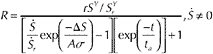 (3) where t = 0 at the time of the step. At t > ta, earthquake rates approach a constant background rate, and at t < ta this solution acquires the form of Omori’s aftershock decay law (Equation 2.8): (4) with p = 1, a = rta, and c = ta exp (–?S/As). Model predictions of aftershock rates, time-dependent expansion of the aftershock zone, proportionality of aftershock duration ta to the inverse of stressing rates, and spatially averaged aftershock decay by t–0.8 all appear to be consistent with the data.2 Variations of this approach have been used to model foreshocks3 and the statistics of earthquake pairs. Recently the state-dependent seismicity formulation has been used to invert earthquake rate for the changes in stress that drive earthquakes at Kilauea, Hawaii.4 |
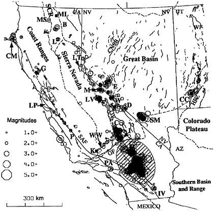
FIGURE 5.2 Map of the western United States showing areas of increased seismicity dynamically triggered by seismic waves from the 1992 Landers earthquake. SOURCE: D.P. Hill, P.A. Reasenberg, A. Michael, W. Arabaz, G.C. Beroza, J.N. Brune, D. Brumbaugh, S. Davis, D. DePolo, W.L. Ellsworth, J. Gomberg, S. Harmsen, L. House, S.M. Jackson, M. Johnston, L. Jones, R. Keller, S. Malone, S. Nava, J.C. Pechmann, A. Sanford, R.W. Simpson, R.S. Smith, M. Stark, M. Stickney, S. Walter, and J. Zollweg, Seismicity remotely triggered by the magnitude 7.3 Landers, California, earthquake, Science, 260, 1617-1623, 1993. Copyright 1993 American Association for the Advancement of Science.
shock triggering by seismic waves are poorly understood but may involve fluid-rock interactions or triggering of local deformations that produce permanent stress changes after the waves have passed through a region.
Foreshocks Foreshocks are generally thought to arise by one of two mechanisms. The first proposes that a mainshock following a foreshock has an identical origin to that of aftershocks. In this case, earthquake frequency-magnitude statistics predict that occasionally an aftershock will
be larger than the prior event, which by definition makes the prior event a foreshock (37). The other proposed mechanism for foreshocks is that premonitory processes, perhaps the fault creep related to mainshock nucleation, result in stress changes that drive the foreshock process in surrounding areas. Models based on state-dependent earthquake rates indicate that both mechanisms are in general agreement with time and distance statistics of foreshock-mainshock pairs (38).
Short-term clustering, as manifest in foreshock-mainshock pairs and aftershocks, attests to large but transient changes in the probabilities of additional earthquakes that occur whenever an earthquake takes place. The concepts of stress interaction and state-dependent seismicity permit physically based calculations of earthquake probability following large earthquakes (39). This approach has been used to evaluate the changes in earthquake probability that arose as a consequence of stress interactions along the Anatolian fault in Turkey (40) and following the M 6.9 earthquake that struck Kobe, Japan, in 1995 (41).
Accelerating Seismicity and Intermediate-Term Prediction A central issue for earthquake prediction is the degree to which the seismicity clustering can be used to monitor the stress changes leading to large earthquakes. Various studies have shown that large earthquakes tend to be preceded by clusters of intermediate-sized events (42). This increase in seismicity can be fit to a time-to-failure equation in the form of a power law, which is commonly used by engineers to describe progressive failures that result from the accumulation of structural damage (43). The power-law time-to-failure equation is also expected if large earthquakes represent critical points for regional seismicity (44).
As described in Section 5.1, regional seismicity has many of the characteristics of a self-organized critical system, including power-law (Gutenberg-Richter) frequency-size statistics and fractal spatial distributions of hypocenters. However, the near-critical behavior of fault systems is the subject of some debate. If the crust continuously maintains itself in a critical state, as originally proposed by Bak and Tang, then all small earthquakes will have the same probability of growing into a big event. This hypothesis has been used as the physical basis for assertions that earthquake prediction is inherently impossible (45). Alternatively, the crust could repeatedly approach and retreat from a critical state. The working hypotheses for this latter view are (1) large regional earthquakes become more probable when the stress field becomes correlated over increasingly larger distances, (2) this approach to a critical state is reflected in an acceleration of regional seismicity, and (3) a system-spanning event destroys criticality on its network, creating a period of relative quiescence after which the process repeats by rebuilding correlation
lengths toward criticality and the next large event (46). It is the decay of the post-event stress shadows by continuing tectonic deformation that introduces predictability into the system.
The seismic cycle implied by these hypotheses agrees with some important aspects of the data on seismic stress shadows and accelerating seismicity (47). Many issues remain to be resolved, however. Quantitative testing will require precisely formulated numerical models adapted to specific fault networks (i.e., computer simulations with realistic representations of fault and block geometries, rheologies, and tectonic loadings). Such “system-level” models are in the early stages of development. The long-term clustering statistics generated by the models must be understood in terms of the underlying dynamics (48), and these behaviors will have to be evaluated against the extended earthquake records now being provided by paleoseismology (see Section 4.3). The key step is to deploy the models in regulated prediction environments to rigorously test their predictive skill.
Key Questions
-
What are the limits of earthquake predictability, and how are they set by fault-system dynamics?
-
Which aspects of the seismicity are scale invariant, and which are scale dependent? How do these scaling properties relate to the underlying dynamics of the fault system? Under what circumstances is it valid to extrapolate results based on low-magnitude seismicity to large-earthquake behavior?
-
Are there patterns in the regional seismicity that are related to the past or future occurrence of large earthquakes? For example, are major ruptures preceded by enhanced activity on secondary faults, temporal changes in b values, or local quiescence? Can the seismicity cycles associated with large earthquakes be described in terms of repeated approaches to, and retreats from, a regional critical point of the fault system?
-
On what scales, if any, is the seismic response to tectonic loading stationary? What are the statistics that describe seismic clustering in time and space, and what underlying dynamics (e.g., mode-switching) control this episodic behavior? Is clustering observed in some fault systems due to repeated ruptures on an individual fault segment or to rupture overlap from multiple segments? Is clustering on an individual fault related to regional clustering encompassing many faults?
-
What systematic differences in fault strength and behavior are attributable to the age and maturity of the fault zone, lithology of the wall rock, sense of slip, heat flow, and variation of physical properties with depth? Are mature faults such as the San Andreas weak? If so, why?
-
To what extent do fault-zone complexities, such as bends, stepovers, changes in strength, and other “quenched heterogeneities,” control seismicity? How applicable are the characteristic earthquake and slip-patch models in describing the frequency of large events? How important are dynamic cascades in determining this frequency? Do these cascades depend on the state of stress, as well as the configuration of fault segments?
-
How does the fault system respond to the abrupt stress changes caused by earthquakes? To what extent do the stress changes from a large earthquake change nearby seismicity rates and advance or retard large earthquakes on adjacent faults? How does stress transfer vary with time (49)?
-
What controls the amplitude and time constants of the postseismic response, including aftershock sequences and transient aseismic deformations? In particular, how important are the induction of self-driven accelerating creep, fault-healing effects, poroelastic effects (which involve the hydrostatic response of porous rocks to stress changes), and coupling of the seismogenic layer to viscoelastic flow at depth?
-
What special processes occur at borders or transition regions between creeping zones, whether localized on faults or distributed, and fault zones that are locked between seismic events? Do lineations of microseismicity provide evidence for processes along such borders?
-
What part of aseismic deformation on and near faults occurs as episodes of slip or strain versus steady creep?
5.3 FAULT-ZONE PROCESSES
The move toward physics-based modeling of earthquakes dictates that research be focused on relating small-scale processes within fault zones to the large-scale dynamics of earthquakes and fault systems. Earthquakes have many scale-invariant and self-similar features, yet numerical simulations must assume some smallest length scale in a grid or mesh, as well as a shortest time step, in order to discretize the computational problem. The issue then becomes how to refine the discretization adequately so that principal phenomena are represented qualitatively, if not at the quantitatively correct small size scale. There is also the question of whether it is possible to capture the wealth of processes that occur on sub-grid scales through judicious parameterizations. For example, rate- and state-dependent friction laws suggest that processes at a scale smaller than the coherent slip patch size can be swept into the macroscopic constitutive description. This characteristic dimension appears to be a very small, however—on the order of 0.1 to 10 meters (see Section 5.4). Numerical resolution of processes at that size scale is well
beyond the capability of current three-dimensional earthquake simulations (50).
Damage Mechanics
The question of how well earthquakes can be approximated as propagating dislocations on idealized friction-bound fault planes is also tied to the degree of rheological breakdown and damage in regions of significant lateral extent away from the rupture surface. Such damage zones can be investigated on large scales by seismological field experiments using fault-zone trapped waves (51) as well as by gravity and electromagnetic methods (52). On smaller scales, processes of rock failure can be studied in the laboratory and their effects observed by field work on exhumed faults.
Recent years have seen strong focus on the possibilities that fractal and granular aspects might be major parts of the observed complexity of fault systems and of fault-zone response. Nevertheless, over the same time, close geological investigations of exhumed fault zones (53) have strengthened the viewpoint that much of the observed complexity of damage zone and secondary fault structures bordering large-slip faults could indeed be a relatively inactive relic of evolution and that, with ongoing slip accumulation, faults become more like Euclidean surfaces (54). For example, studies at the Punchbowl and North Branch San Gabriel faults (55) show abundant complexity of structure, with damaged and faulted rock that extends on order of 100 meters from the fault core. Yet a severely granulated ultracataclastic core on the order of only 100 millimeters wide seems to have accumulated all significant slip, summing to several kilometers of motion. Also, a principal fracture surface that may be only a few millimeters wide seems to have hosted large amounts of slip, presumably corresponding to the last several earthquakes, whereas there is little evidence of significant slip accumulation on secondary faults in the damaged border zone.
This does not at all imply that the damaged zone is irrelevant to fault dynamics. First, it is a storage site for pore fluids. Second it provides a heterogeneity of elastic properties that may allow slip on the main fault, if not well centered within the damaged zone, to induce changes in normal stress, with consequences for frictional instability (56). Third, as a zone of low strength, it may react inelastically to the high stresses associated with a propagating rupture front. Stresses acting off the main fault plane become much larger than those along it as the rupture approaches what, in elastic-brittle dynamic crack theory, would be its limiting speed (57). It is likely that faulted rock within that border region acts as a macroscale plastic zone when rupture speed approaches the limit speed, so that much of the inferred fracture energy of earthquake faulting may emanate from
energy dissipation in the damage zone rather than exclusively from the main fault surface itself (as often assumed in relating seismic observations to parameters of slip-weakening rupture description). Also, the high off-fault stresses may activate rupture along fortuitously oriented, branch fault structures that intersect the main fault. Such a process is a possible source of spontaneous arrest of rupture and of intermittence of rupture propagation speed (enriching the radiated seismic spectrum at high frequencies), and it can be correlated to natural examples of macroscopic branching of the rupture path (58).
Friction of Fault Materials
Experimentally determined constitutive laws, such as those presented in Box 4.4, have been validated for slip rates between about 10–10 and 10–3 meter per second. As such, they cover the range from plate rates to rates at which incipient dynamic instabilities are well under way, so they probably provide an appropriate description of frictional processes during earthquake nucleation and postseismic response. In the common form of these laws, the logarithmic dependence of stress on sudden changes in sliding velocity, introduced empirically, is now generally assumed to descend from an Arrhenius activated rate process governing creep at asperity contacts (59). That is, the slip rate V for each active mechanism at the contacting asperities is proportional to e–Q/RT, where the activation energy Q is diminished linearly by stress over the narrow range sampled in experiments. This leads at once to the instantaneous ln V dependence of friction coefficient in the range for which forward-activated jumps are vastly more frequent than backward ones. Considering the backward jumps regularizes the ln V dependence at V = 0 (60). Experiments on optically transparent materials, including quartz, have linked the state evolution slip distance Dc to the sliding necessary to wipe out the original contact population and replace it with a new one (61). These experiments also showed time-dependent growth of contact junctions, which is a mechanism by which strength depends on the maturity of the contact population (measured by the state variable). Further, models have proposed thermally activated creep as a mechanism for contact growth that delivers a steady-state friction coefficient proportional to ln V (62), which is often observed, at least over limited ranges, in experiments.
The above description outlines the simplest physical understanding of the empirically derived friction laws. To confidently extend these relations to situations not directly studied in the laboratory, it will be important to put them on a firmer basis, in a way that deals more completely with contact statistics and the actual granular structure of fault-zone cores and that recognizes the possibility of multiple deformation mechanisms
with different dependencies on temperature, stress, and the chemical environment. A simple version is to assume that deformation in the fault zone can include both slip on frictional surfaces and more distributed creep deformation, with both processes taking place under the same stress (63). Based on earlier hydrothermal studies of granite and quartz gouge (64), F. Chester suggests that response can be modeled by three mechanisms: solution transfer, cataclastic flow, and localized slip (65). Each is assumed to follow a rate- and state-dependent law, but with additional terms to represent effects of changing temperature. Studies of this kind, firmly rooted in materials physics, are needed to extrapolate laboratory data confidently over a range of hydrothermal conditions to very long times at temperature on natural faults, to infer in situ stress conditions and the conditions of local stress and slip rate necessary to nucleate a frictional instability.
Earthquake Mechanics in Real Fault Zones
It may be conjectured that different physical mechanisms prevail at contacts during the most violent seismic instabilities, when average slip rates reach 1 meter per second and maximum slip rates near the rupture front might be as great as 102 meters per second. In that range, the dynamics of rapid stress fluctuations from sliding on a rough surface, openings of the rupture surfaces, microcracking, and fluidization of finely comminuted fault materials may result in a different velocity dependence, possibly with a dramatic weakening. Most significantly, very large temperatures will be generated in the rapid, large slips of large earthquakes. These are expected to lead to thermal weakening, but there is presently very limited laboratory study of the process (66). When two surfaces slide rapidly, compared to heat diffusion times at the scale of the asperity contacts, a first thermal weakening is due to flash heating and thermal softening of the contacts (67). With poor conductors such as rocks, continued shear—especially along narrow surfaces as inferred for the Punchbowl fault (68)—would necessarily lead to local melting. The amount of melt generated in actual faulting events is not well constrained. Pseudotachylytes (amorphous rocks, rapidly cooled from the melt) are sometimes seen as fillings of faults and of veins that run off them and at dilatational jogs (69). An open question is, how much of the finest-grain gouge components are also the result of rapid cooling of a melt that has been squeezed into narrow pore spaces where it solidified and thermally cracked to small fragments upon cooling.
Although there are presently few experimental constraints on response in the high-slip-rate range, experiments and coordinated theory for this range are essential to understanding the overall stress levels at
which faults operate, the heat outflow from faults (and whether its lowness is paradoxical or not), and the mode of rupture along them. For the latter, it is now understood (70) that strong velocity weakening together with low shear stress levels over the region through which a rupture propagates promote self-healing of the rupture behind the front, a phenomenon found in numerical simulations (71) and observed in real events (72). Yet whether it is velocity weakening or some other process or fault-zone property that controls the observed mode of rupture remain to be clarified. Good experiments and observations are a must, and velocity-weakening constitutive response is not the only route to short slip duration. They can also be induced by strong fault heterogeneity (73) and as a consequence of even fairly modest dissimilarity of elastic properties between the two elastic blocks bordering a fault zone (74).
Provided that typical laboratory friction coefficients for rocks (0.5 to 0.7) apply and that pore pressure is hydrostatic, the shear strength that must be overcome to initiate slip at, say, 10-kilometer depth is estimated to be about 100 megapascals. This is much larger than seismic stress drops, typically on the order of 1 to 10 megapascals. Thus, one option is that faults slide during large earthquake slips at stresses on the order of 100 megapascals. This is, however, in conflict with the well-known lack of a sharply peaked heat outflow over the San Andreas fault (see Section 2.5). It is also difficult to reconcile with observations (75) of a steep inclination (60 to 80 degrees) with the San Andreas fault of the principal compression direction in the adjoining crust. The possible ways around this problem are the subject of much discussion. It has been argued (76) that the heat flow data are unreliable, being influenced by shallow topographically driven groundwater flows, and that stress directions are dictated by bordering tectonics and are a misinterpreted signal of tectonics in the bordering regions. However, many workers have not been as ready to dismiss these considerations and have sought other modes of explanation. Pore pressure that is greatly elevated over hydrostatic, and nearly lithostatic, at seismogenic depth has been invoked. Also, the possibility has been raised that fault-zone material within well-slipped faults has anomalously low friction, due either to its mineralogical or its morphological evolution (e.g., possibly stabilizing hydrophilic phases with low friction comparable to that of montmorillonite clay (77)) or to the inclusion of weak lithologies, possibly serpentine, in the fault. In contrast to these propositions for zones of active tectonics such as the San Andreas, faults intersected by the few deep drill holes in stable continental crust seem to be at hydrostatic pore pressure and to carry maximum shear stresses consistent with friction coefficients in the range 0.5 to 0.7 (78). Thus, it is important to better constrain these possibilities
by drilling, such as that planned in the San Andreas Fault Observatory at Depth (SAFOD) component of the EarthScope Program, as well as by examinations of exhumed faults, to establish if and why major plate-bounding faults are different in composition or fluid pressurization.
Yet another possibility is that dynamic weakening may be responsible for the low-stress observations along the San Andreas fault. Sources could include severe thermal weakening, including melt formation, in rapid, large slips, as above, or the formation of gouge structures that accommodate slip by rolling with little frictional dissipation (79). In the case of sliding between elastically dissimilar materials, there is coupling between spatially inhomogeneous sliding and alteration of normal (clamping) stress. Mathematical solutions have been constructed that allow a pulse of slip to occur in a region of locally diminished clamping stress and hence diminished frictional dissipation (80). Experiments on foam rubber blocks (81) show a similar effect, even leading to surface separation. Analogous effects have not been found in laboratory rock experiments in the large sawcut apparatus at the U.S. Geological Survey (USGS)-Menlo Park, and the mechanism in the foam rubber remains obscure (nonlinearities in the surrounding continuum-like field could contribute); however, something similar to this could be found for natural faults, possibly as a result of the interaction of the fault core with the damaged zone adjoining it.
These considerations highlight the importance of determining the composition, structure, and physical state of fault-zone materials; of determining their rheology, especially in rapidly imposed large slips; and of understanding the dynamical processes within the core and their interaction with the heterogeneity and possible localized failure processes in the damaged border zones. At larger scales, there is a need for better characterization of fault junctions and of the structure and mechanical properties of fault-jog materials, over or through which rupture jumps in transferring slip from one fault segment to another.
Key Questions
-
Which small-scale processes—pore-water pressurization and flow, thermal effects and melt generation, geochemical alteration of minerals, solution transport effects, contact creep, microcracking and rock damage, gouge comminution and wear, gouge rolling—are important in describing the earthquake cycle of nucleation, dynamic rupture, and postseismic healing?
-
What fault-zone properties determine velocity-weakening versus velocity-strengthening behavior? How do these properties vary with temperature, pressure, and composition?
-
What rheologies govern the shallow deformation of fault zones? When does fault creep occur near the surface? Do lightly consolidated sediments allow distributed inelastic deformation?
-
How does fault strength drop as slip increases immediately prior to and just after the initiation of dynamic fault rupture? Are dilatancy and fluid-flow effects important during nucleation?
-
What is the nature of near-fault damage and how can its effect on fault-zone rheology be parameterized? Can damage during large earthquake ruptures explain the discrepancy between the small values of the critical slip distance found in the laboratory (less than 100 microns) and the large values inferred from the fracture energies of earthquakes and assumptions about the drop from peak strength for slip initiation to dynamic friction strength (5 to 50 millimeters if the strength drop is 100 megapascals, but an order of magnitude higher for 10 megapascals)?
-
Are the broad damage zones observed for some faults relics of the evolution of a through-going fault system on what was a misoriented array of poorly connected fault segments that were reactivated or originated as joints? Do the damage zones result from misfit stresses generated by the sliding of surfaces with larger-scale fractal irregularities? Are they just passive relics or do they also play a significant role in the dynamics of individual events?
-
How does fault-zone rheology depend on microscale roughness, mesoscale offsets and bends, variations in the thickness and rheology of the gouge zone, and variations in porosity and fluid pressures? How can the effects of these or other physical heterogeneities on fault friction be parameterized in phenomenological laws based on rate and state variables?
-
How does fault strength vary as the slip velocities increase to values as great as 1 meter per second or more? How much is frictional weakening enhanced during high-speed slip by thermal softening at asperity contacts and by local melting?
-
How do faults heal? Is the dependence of large-scale fault healing on time logarithmic, as observed over much shorter times in the laboratory? What small-scale processes govern the healing rate, and how do they depend on temperature, stress, mineralogy, and pore-fluid chemistry?
-
How does rupture on a major fault interact with faults in the bordering regions? Is this interaction a source of intermittent rupture propagation and resulting enriched high-frequency radiated energy or of the spontaneous arrest of ruptures? Are the high seismically inferred fracture energies (on the order of 100 times laboratory values for initially intact rock under high confining stress) actually due to induction of extensive frictional inelasticity in that border zone? Is fracture energy misinter-
-
preted as being due to slip weakening on a single major fault versus a network of dynamically stressed secondary faults?
-
When does the rupture path follow a fault that branches off from the major failure surface? What is the role of pre-stress magnitudes and orientations and of the dynamically altered stress distribution near the rupture front? How do ruptures surmount stepovers? Are elastic descriptions adequate for the stepped-over material, or is there an essential role for damaged rock and smaller fault structures within the stepover region?
5.4 RUPTURE DYNAMICS
Earthquake rupture entails nonlinear and geometrically complex processes near the fault surface, generating stress waves that evolve into linear (anelastic) waves at some distance from the fault. Better knowledge of the physics of rupture propagation and frictional sliding on faults is therefore critical to understanding and predicting earthquake ground motion. Research on rupture processes may also contribute to improvements in earthquake forecasting because of the dynamical connection between the evolution of the stress field on interseismic time scales and the stress heterogeneities created and destroyed during earthquakes.
Rupture Initiation
The process leading to the localized initiation of unstable stick-slip in laboratory (82) and theoretical (83) models of the earthquake process is referred to as earthquake nucleation. In frictional fault models, stick-slip instabilities can begin only in regions where the progression of slip causes the fault friction to decrease. For the rate-state model, this situation corresponds to velocity weakening—when the steady-state friction µss decreases with velocity V:
(5.1)
The dimensionless rate dependence a – b can vary with rock composition, temperature, and pressure. Equation 5.1 defines the condition at which earthquake nucleation can occur (Figure 4.30). However, a correspondence between the depth range at which earthquakes occur and the region where a – b is negative has not been confirmed by independent observations of velocity weakening, and there is no micromechanical theory that can be used to extrapolate laboratory data to crustal conditions. Nevertheless, the available lab information on the effect of temperature on the constitutive parameters, combined with inferred geotherms, suggests
a reasonable degree of agreement between the depth at which a – b is expected to become positive and the depth at which earthquakes stop.
As a fault is loaded, stress will fluctuate about the quasi-steady value tss = µsssn. Where stress is a bit higher than tss, the slip rate increases slightly and occasionally a fluctuation will occur over a large enough area to initiate an instability. The criterion for instability is that the patch size be larger than a critical value Lc:
(5.2)
where G is the shear modulus. As nucleation begins, slip concentrates within a region of characteristic dimension Lc, and slip rate increases inversely with the time to instability (Figure 5.3). To what extent this type of behavior occurs in the Earth and what the size of Lc might be are two of the key questions in the science of earthquakes.
Earthquake nucleation is difficult to observe on faults in the Earth for two reasons. First, it is predicted to occur only over a spatially limited nucleation zone. If this zone is small, it will be difficult to detect. Second, nucleation may be a largely aseismic process such that it will not generate seismic waves. There are, however, observations that constrain possible models of earthquake nucleation, and these can be grouped into two classes: those that suggest the nucleation zone is small and those that suggest the nucleation zone is large.
Several types of observations point to a small nucleation zone (Lc less than 100 meters). Borehole strainmeter data provide the most sensitive measurements of small strain signals in the near field. These data show no evidence of strain precursors at levels that correspond to about 1 percent of the mainshock seismic moment (84). This suggests that the nucleation zone and the amount of slip within it must be small (Figure 5.4). A second line of evidence comes from rupture dimensions of the smallest earthquakes, which place an upper bound on the size of the nucleation zone since slip over an area less than Lc must be stable. Microearthquakes on the San Andreas fault recorded on the downhole instruments of the deep Cajon Pass borehole have source dimensions of about 10 meters (85). This places an upper bound on the size of the nucleation zone, at least locally, though fault roughness, gouge thickness, and apparent normal stress all affect Lc and will vary spatially. If the laboratory parameters for smooth faults applied to faults in nature, the minimum earthquake size would be on the order of 1 to 10 meters. Direct evidence for a lower-magnitude cutoff at the upper end of this range (near M 0) comes from the microseismicity observed by sensitive networks in the deep gold mines of South Africa (86).
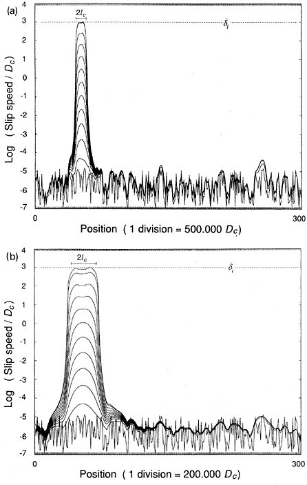
FIGURE 5.3 Numerical simulation of earthquake nucleation on a fault governed by rate-state friction with A = 0.004, B = 0.006, ? = 109 s, G = 104s, t = 0, and initial shear stress from (µ’0 + 0.06)s to (µ’0 + 0.08)s. The fault is discretized with 300 elements and initialized with random stress fluctuations. Lines show the slip speeds at successive times in the calculation; the time intervals are decreased by one order of magnitude for every order-of-magnitude increase in slip velocity. SOURCE: J.H. Dieterich, Earthquake nucleation on faults with rate- and state-dependent strength, Tectonophysics, 211, 115-134, 1992. With permission from Elsevier Science.
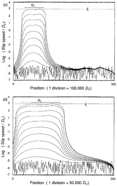
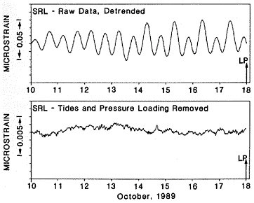
FIGURE 5.4 Preseismic strain observations of the 1989 Loma Prieta earthquake as recorded at San Juan Bautista. Upper panel shows a week of dilational strains with the oscillatory solid Earth tides. The lower plot presents the same record with Earth tides and atmospheric loading removed. The absence of a preseismic signal constrains the moment magnitude of an aseismic precursor to be no more than M 5.3, or less than 1 percent of the mainshock seismic moment. SOURCE: M.J.S. Johnston, A.T. Linde, and M.T. Gladwin, Near-field high-resolution strain measurements prior to the October 18, 1989, Loma Prieta Ms 7.1 earthquake, Geophys. Res. Lett., 17, 1777-1780, 1990. Copyright 1990 American Geophysical Union. Reproduced by permission of American Geophysical Union.
Several lines of evidence argue for a large nucleation zone (Lc greater than 100 meters). The low-frequency spectra for some earthquakes show a slow component that may precede the first detectable high-frequency waves by tens of seconds (87). For these events, there may be a gradual transition from aseismic nucleation to unstable rupture (88) (Figure 5.5). The character of the onset of microearthquakes suggests that very small events also begin with a slow onset that scales in duration with the overall source duration (89). The first arriving seismic waves of moderate to large events in the near field often show an initial phase of irregular growth (90). The duration of this phase shows a similar scaling with earthquake size as reported for the slow initial phase (Figure 5.6). If this phase represents the tail end of a process that is otherwise aseismic, then the dimensions of the nucleation zone are substantial.
Foreshocks provide the clearest evidence of a preparation process before at least some earthquakes. Approximately 40 percent of earthquakes
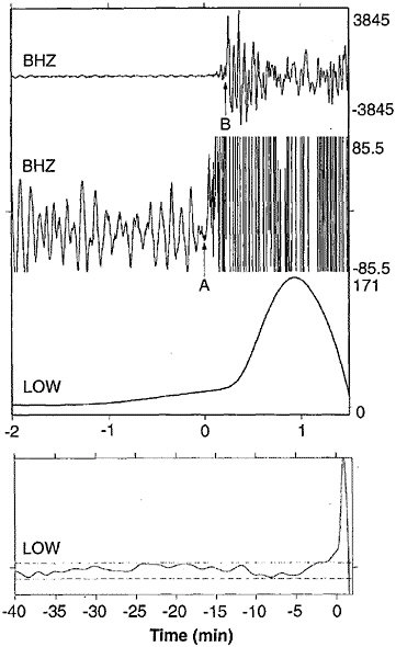
FIGURE 5.5 Vertical component P-wave seismograms from the 1994 Romanche Transform earthquake at low-noise GEOSCOPE station TAM. Top two panels show broadband trace at two magnifications and third panel shows a detided, low-pass filtered version of the same data revealing the precursory ramp beginning at least 1 minute before the high-frequency origin time. Lowermost panel shows filtered, detided data at a longer time scale indicating that the signal emerges from the background noise level (dashed lines). SOURCE: J. McGuire, P. Ihmle, and T. Jordan, Time-domain observations of a slow precursor to the 1994 Romanche Transform earthquake, Science, 274, 82-85, 1996. Copyright 1996 American Association for the Advancement of Science.
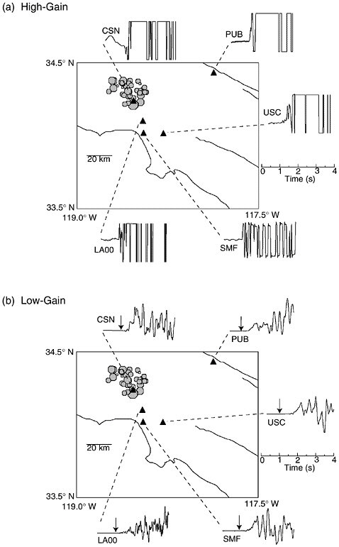
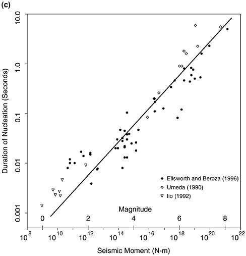
FIGURE 5.6 Left two panels show map view of the Northridge mainshock and aftershocks as filled octagons, with seismic stations as triangles. (a) Vertical component velocity seismograms of the initial P waves of the Northridge mainshock. SMF is a high-gain record that quickly clips, while the other traces are artificially clipped to simulate limited dynamic range recording and to show that the onset of the first P wave at this scale is abrupt. (b) Low-gain recordings of the initial P waves of the Northridge mainshock at the same sites. In each case the arrow indicates the first arriving waves shown in the upper panel. The onset, though abrupt, remains weak until about 0.5 second into the mainshock. Similar behavior is observed before other earthquakes. (c) The duration of the weak initial onset, or seismic nucleation phase, for earthquakes from several studies indicates that the seismic nucleation phase (vertical axis) scales with the seismic moment (horizontal axis) of the mainshock. SOURCE: G.C. Beroza and W.L. Ellsworth, Properties of the seismic nucleation phase, Tectonophysics, 261, 209-227, 1996. With permission from Elsevier Science. (c)
are preceded by at least one observable foreshock (91). Foreshock sequences are more common and are more protracted for earthquakes initiating at shallow depths, which is consistent with an expected decrease in frictional stability with decreasing normal stress (92). Foreshock frequency is observed to increase as t–1, where t is the time before the mainshock (93). In at least some cases, foreshock sequences were unlikely to have triggered the mainshock (94). Instead, some other process, such as aseismic nucleation, may have driven both the foreshocks and the mainshocks to failure.
Earthquake nucleation may hold the key to whether or not earthquakes are predictable over the short term. If nucleation is so unstable that any small event could cascade into a large earthquake, then the prospects for deterministic earthquake prediction are grim because one would have to predict both the small initial earthquake and the fact that conditions would cause it to grow into a large earthquake. If, on the other hand, the nucleation process scales with earthquake size, the prospects for earthquake prediction are brighter. It is possible, even likely, that different faults will manifest different behaviors, with some (e.g., oceanic transforms) having different nucleation behavior than others. Understanding the nucleation process will require sensitive observations as close as possible to areas of likely earthquake initiation for a range of fault types and a number of large events. Current observational programs, with the exception of the Parkfield experiment (Section 2.6), are not designed to detect such phenomenon at the likely initiation points of significant events.
Rupture Propagation
Once nucleation occurs, rupture can propagate and expand in an earthquake. The mechanics of rupture propagation are complex and poorly understood for several previously discussed reasons. First, it is challenging to design laboratory measurements at the high sliding velocities and large displacements found in earthquakes. Second, physical phenomena that may be unimportant while the fault is locked or sliding slowly, such as shear heating of pore fluids or melting of fault-zone minerals, can become critically important at high slip speeds. Finally, in the near field, where the potential to make unobscured observations of the earthquake rupture process is highest, strong ground motion drives most seismic instrumentation off-scale. These factors have conspired to impede progress in understanding the mechanics of earthquake rupture; nevertheless, such an understanding is central to many of the most important goals of earthquake science, such as predicting the level and variability of strong ground motion, characterizing the nature of large earthquake recurrence, and understanding the extent to which earthquakes might be predictable.
The dynamics of earthquake rupture are usually described in the terminology of fracture mechanics (95). A common application of crack models to earthquake studies is to define relationships between seismological observations and dynamical parameters. The average offset on a fault u and its characteristic dimension L are related to the static stress drop ?s by the formula ?s = csGu /L, where cs is a constant determined from crack theory, which depends on the fault type. In crack theory, the rupture velocity is a function of the fracture energy near the crack tip (96). The exact relationship depends on the crack geometry, but in general, rupture speed increases as the fracture energy decreases. The rupture velocity is generally much faster than the fault’s particle velocity, the speed with which one side of the fault moves with respect to the other; typical values are 2 to 3 kilometers per second and 0.3 to 2.0 meters per second, respectively. The particle velocity can be related to the tectonic stress s0 driving the fault motion. Since fault motion is impeded by a frictional stress sf, the actual stress available for driving fault motion is the difference, se = s0 – sf, called the dynamic stress drop. The particle motion velocity V is given by cdßse/G, where ß is the shear velocity, G is the rigidity, and cd is a constant determined by the geometry of the fault. Particle velocities of about 1 meter per second imply that se is of the order of 100 bars, or 10 megapascals (97).
Crack models are useful but must be applied with caution. The rupture velocity of large earthquakes is rarely constant and faults may rupture in a stop-and-go fashion. Cracks in ideally brittle materials have stress concentrations that are infinite at the sharp crack tip. In real materials, nonlinear deformations such as plastic flow eliminate this singularity by distributing the stress over a finite process zone. Various models have been advanced to describe this behavior (98), though their dynamical effects can usually be lumped into an effective value of Kc. This nonideal version of the critical stress intensity factor defines a material parameter called the fracture toughness.
Two main difficulties are encountered in the application of idealized crack mechanics to the earthquake problem. One lies in the assumption that the crack is cohesionless behind the crack tip, which implies that the stress drop during fracture is complete. On real faults, shear motion is impeded by friction, so that the stress drop is incomplete; in fact, the work against friction during fault slip turns out to be the dominant term in the energy balance. The second problem is the ad hoc treatment of what happens in the process zone at the edge of the crack, where an attempt must be made to stitch together two fundamentally different ways of describing material behavior, from the bulk rheology that governs the unfractured rock ahead of the crack tip to the surface friction that applies
once the fracture has passed by. In these respects, the view of earthquakes as frictional instabilities is more appropriate.
An important research area is how ruptures in earthquakes compare with idealizations of rupture based on fracture mechanics. The notion that rupture in earthquakes propagates outward from the hypocenter was implicit in the recognition that earthquakes are caused by shear slip on faults, but it was not until the 1950s that the effects of rupture propagation on seismograms were first identified (99). Teleseismic and near-source estimates of average rupture velocity are consistently in the range of about 70 to 90 percent of the S-wave velocity (100). There is no evidence that rupture velocity varies with magnitude, from the very largest earthquakes to the very smallest earthquakes for which it can be determined (101). Rupture velocities that are a large fraction of the shear-wave velocity lead to pronounced directivity in strong ground motion, particularly for shear waves (102).
It is not clear why earthquakes should rupture at these velocities. The simplest models based on elastic-brittle fracture mechanics for a preexisting planar fault suggest that shear rupture ought to accelerate very quickly to a limiting velocity that depends on the mode of rupture: either the shear-wave velocity for antiplane rupture or the Rayleigh-wave velocity (about 92 percent of the shear-wave velocity) for in-plane rupture (103). The same models, predict that stresses for out-of-plane rupture will grow as the limiting velocity is approached, which should promote rupture bifurcation and a lower rupture velocity. For the most part, rupture is observed to propagate at velocities slightly below the limiting velocity for the elastic-brittle case. There are, however, important exceptions to this behavior.
Rupture velocity has locally exceeded the S-wave velocity for at least several earthquakes (104). Such supershear rupture velocities are expected in models that incorporate a process zone that fails under finite cohesive traction (105), and they have been observed recently in laboratory fracture experiments (106). If supershear rupture propagation should prove common, however, it would have important implications for strong ground motion. During an episode of supershear rupture propagation, an earthquake will form a Mach cone, the seismic equivalent of a sonic boom, but in the case of earthquakes, a high-amplitude wavefront will result (107), with the potential to contribute substantially to the level of damaging strong ground motion.
Slow earthquakes are seismic events for which the rupture and/or slip velocities are unusually low. They are identifiable by unusually strong seismic wave excitation at long periods (108). An important class of slow earthquakes is tsunami earthquakes, which generate tsunamis far larger than expected based on their magnitude (109). The devastation wrought
by tsunami earthquakes can be extreme (110). Moreover, near the tsunamigenic source, there is little time for warning. Because of their tremendous destructive potential, it is extremely important to understand why such earthquakes occur. More generally, slow earthquakes are known to occur in many tectonic environments (111), but they are particularly common on oceanic transform faults. The fact that slow earthquakes are particularly common on transforms where sedimentary cover is negligible precludes rupture through, or slumping of, mechanically weak sediments as a uniform explanation for slow events. Their association with oceanic transforms may instead be related to properties of the relatively young, hot, and thin oceanic crust (112).
Silent earthquakes are slip episodes that occur so slowly that they do not generate short-period seismic waves and hence are not earthquakes in the usual sense of the word. The largest known silent earthquake was a precursor to the 1960 Chile earthquake. The slow component of this event at M 9.3 is larger than any other recorded earthquake except for the 1960 M 9.5 Chile mainshock that followed it. Because it did not radiate high-frequency seismic waves, the precursor was not even recognized until more than a decade later (113). There are now several spectacular examples of large silent earthquakes in Japan (114), as well as smaller silent earthquakes on the San Andreas fault system (115). A study of the Earth’s longest-period free oscillations found excitations of the Earth’s free oscillations that were not accounted for by known earthquake activity (116). More recently, it has been found that the Earth’s free oscillations are continuously excited (117), although it is not yet clear what the source of this excitation is. If it is earthquake activity, then it requires a substantial revision of our view of faulting. Episodic slip would have to be common and more or less continuously occurring somewhere in the world. The source of continuous excitation could also be atmospheric, which if true offers new possibilities in seismology on other bodies of the solar system (118).
Fault creep, the steady motion of a fault without generation of seismic waves, can be episodic at the Earth’s surface and occur in discrete events (119), but its behavior at depth is less well known. Some faults such as parts of the San Andreas, Hayward, and Calaveras faults in California seem to be creeping aseismically (120). Aseismic creep has also been called upon to explain postseismic deformation transients (see Section 4.2). It has long been known that seismicity on many of the Earth’s major fault systems is insufficient to keep up with the rates of slip predicted from plate tectonics (121). To what extent this aseismic slip occurs continuously versus episodically remains an open question.
Another important aspect of earthquake rupture propagation is the rise time—the duration of slip at a point on the fault. The rise time has
been determined for a few earthquakes for which adequate near-source strong-motion data are available (122), but for most large earthquakes the rise time is unresolved (123). If one supposes that the fault will not stop sliding until it receives information that allows it to heal from the farthest reaches of the fault plane (124), then the rise time should be proportional to the spatial extent of the fault. The rise time is much shorter than would be predicted given the length of the fault, and in some cases it is shorter than the width of the fault would predict as well (125).
Explanations for short rise times can be characterized as either dynamic or geometric. Dynamic explanations center on the notion that if the velocity dependence of friction is strong enough, it might lock the fault as the sliding velocity decreases, well before information propagates inward from the fault edges (126). Geometric explanations focus on smaller length scales in the faulting process, due to geometry or material properties of the fault that might cause the rise time to be short. In this case the rise time may be controlled by the dimension of the high-slip regions, rather than the overall fault dimensions. Quasi-dynamic models of earthquakes (127) support this point of view.
Whatever their cause, the combination of short rise time and high rupture velocity leads to strong shear-wave arrivals of short duration in the near field in which a broad range of frequencies arrive in phase. The strong pulse that results poses challenges for earthquake engineering (128), so that it is critical to determine what controls the behavior of these aspects of rupture propagation. Because our understanding of strong ground motion is based primarily on a limited number of moderate earthquakes (M < 7.0), an increased understanding of the factors that control strong ground motion, such as the rise time, is essential in efforts to extrapolate observations of strong ground motion in moderate earthquakes to larger earthquakes.
Slip on faults during earthquakes is known to be spatially variable. Early representations of earthquake sources as multiple point sources were motivated by observations that earthquakes are punctuated by a series of subevents that radiate energetically (129). A more general characterization of heterogeneity represents an earthquake by a continuous distribution of slip in space and time. This approach cannot be applied in a meaningful way to most earthquakes because of insufficient resolution (130); however, in the near field where high-frequency waves are not greatly attenuated and Green’s functions vary strongly with position, detailed source imaging is possible. Extended-source models of rupture for several dozen earthquakes have been derived from strong-motion data (131) and show that both slip and rupture velocity in earthquakes are strongly heterogeneous in both space and time (132) (Figure 4.7).
Most extended-source models are kinematic in the sense that the slip
distribution is specified without considering the stress on the fault and the fault-constitutive behavior it implies. Dynamic models explicitly account for the stress and attempt to characterize the behavior of the fault in terms of simple physical laws. One approach to reconcile kinematic and dynamic rupture modeling is termed quasi-dynamic modeling, in which dynamic rupture models are developed that reproduce kinematic models (133). Because modeling strong-motion and other data in quasi-dynamic models is indirect, there is no guarantee that the model will be consistent with the original data. A goal for the future is to estimate dynamic parameters directly from strong-motion data. Preliminary work in this area suggests that some dynamic parameters such as the slip weakening distance may be very difficult to resolve from surface measurements (134). Short of complete dynamic modeling, one can also recover aspects of fault rupture dynamics without developing a dynamic rupture model for the entire event (135).
It has long been recognized that earthquake rupture must be heterogeneous at small scale lengths to explain observed high-frequency ground motion (136). The acceleration spectra of earthquakes is observed to be constant above the corner frequency. Models of constant slip with smooth rupture propagation result in acceleration spectra that decay above the corner frequency (137) unless seismograms are dominated by the effects of rupture termination (138). A number of models have been developed to explain this observation (139). Seismologists have known that heterogeneous rupture should lead to enhanced radiation at frequencies of concern to earthquake engineering (140). There is now evidence to confirm this hypothesis. Areas of strong high-frequency generation are observed to correlate with areas of strong slip variations (141), and there are stochastic models of earthquake rupture that lead to realistic strong ground motions (142).
Rupture Arrest
Rupture will propagate along a fault in an earthquake until something stops it. For large earthquakes, the depth extent of seismic rupture is bounded from below by the depth of the transition from brittle to ductile behavior (143) and from above by the Earth’s surface (144). What controls the horizontal extent of rupture in large earthquakes, or the spatial extent of smaller earthquakes that terminate before they reach the edges of the seismogenic zone, is less clear. Factors likely to influence the extent of rupture include fault geometry, variation of material properties, and stress heterogeneity.
The irregularities in geometry that occur at all scale lengths (145) have the potential to exert a strong control on earthquake rupture for earth-
quakes of all sizes (see Figure 3.2). At the surface, fault-zone irregularities can be mapped geologically. Such irregularities, particularly fault discontinuities, across which slip transfers from one surface to another, are thought to play an important role in controlling the maximum earthquake size on a particular fault system (146). This idea is supported by studies of fault segmentation as expressed both in surface faulting and in aftershock distributions (147). There are, however, clear observations of earthquakes that were not terminated by fault-zone discontinuities (148). The Landers earthquake provides a spectacular example (149). This earthquake started on the Johnson Valley fault and ruptured primarily to the north, then jumped across a discontinuity to the Homestead Valley fault and continued to rupture northward. It then jumped across yet another discontinuity and ruptured northward on the Emerson fault before stopping in the middle of a relatively straight fault segment. Given the potential utility of using fault segmentation to anticipate earthquake size, it is important to determine under what conditions a propagating rupture such as this will or will not jump from one fault segment to another. The ability to model the conditions under which an earthquake that ruptures toward a fault jog will terminate or breach the jog and continue to grow into a larger earthquake can help anticipate the size of future earthquakes. The possibility of multiple-segment ruptures has been included explicitly in assessments of earthquake probabilities in California (150).
One factor that determines how effectively a discontinuity will act to limit fault rupture is the distance between the offset fault segments. Empirical observations suggest that fault discontinuities with less than 1 kilometer of offset do not pose a strong impediment to rupture; whereas discontinuities with 1- to 5-kilometer offset terminated rupture some of the time, and discontinuities with offsets of 5 kilometers or more always terminated rupture (151). Two-dimensional numerical models of dynamic rupture interacting with a fault discontinuity are consistent with these observations (152).
Another factor is the sense of the discontinuity (i.e., whether a jog in a fault leads to extensional or compressional strains). Compressional jogs are more difficult to propagate across, because the normal stress will increase and because uplift to accommodate compressional strain within the jog will have to be done against gravity (153). Finite-difference modeling suggests that earthquakes are unlikely to propagate across compressional jogs with offsets greater than 3 kilometers or extensional jogs with offsets greater than 5 kilometers (154). Three-dimensional modeling of rupture across a fault discontinuity has refined the ability to model why some earthquakes terminate at segment boundaries while others cascade into multisegment ruptures and hence much larger earthquakes.
Variations in material properties may also exert a control on the extent of rupture in earthquakes. This is certainly true in the grossest sense at the brittle-ductile transition and at the Earth’s surface, but variations in material properties may also be important either in the material adjacent to the fault or within the fault zone itself. There is strong evidence that material properties near the Earth’s surface control rupture propagation through the shallowest layers (155). Further evidence that material in the vicinity of the fault zone may help control earthquake size comes from tomographic studies of velocity variations in the vicinity of recent large earthquakes (156). A possible interpretation is that these areas of the fault accumulate shear stress, while parts of the fault that are bordered by lower-velocity material may slip aseismically.
The observation that the creeping section of the San Andreas and Calaveras faults in California have areas of micro-earthquake activity interspersed with small zones that fail repeatedly in small earthquakes (157) suggests that material variations may cause some parts of the fault surface to fail in stick-slip while the rest of the fault creeps (158).
Accumulated stress is the fuel that provides the energy for earthquake faulting, and variations in stress may play an important role in controlling earthquake size. Rupture may stop when it propagates into a region that has very little pre-stress. Such a stress barrier is a means of terminating rupture (159) and is implicit in the stuck patch (160) or asperity model of earthquake behavior (161), in which highly stressed parts of the fault fail at high stress drop and the rupture stops within lower-stress areas on the surrounding fault. The termination of rupture on the Emerson fault in the Landers earthquake may provide an example of a rupture that stopped owing to low stress on the fault before the mainshock rupture (162). If the Emerson fault was far from failure before the Landers mainshock, then it may have terminated at shallow depth with rupture nucleating at shallow depth, but not propagating to greater depths or farther along the fault (Figure 5.7).
Understanding the factors that control the extent of earthquake rupture is extremely important. Fault geometry, material property variations, and stress variations, are all likely to play an important role. Moreover, these factors are interdependent, and it may be impossible to fully disentangle the effects of one from the others. The 1934 and 1966 Parkfield earthquakes illustrate this. The 1934 earthquake apparently did not rupture past the extensional fault jog in Cholame Valley, whereas the 1966 Parkfield earthquake did (163). The geometry did not change between 1934 and 1966; perhaps the fault jog was sufficient to terminate rupture in 1934, but not in 1966, because the fault to the south of the jog was closer to failure before the 1966 event than it was before the 1934 event.
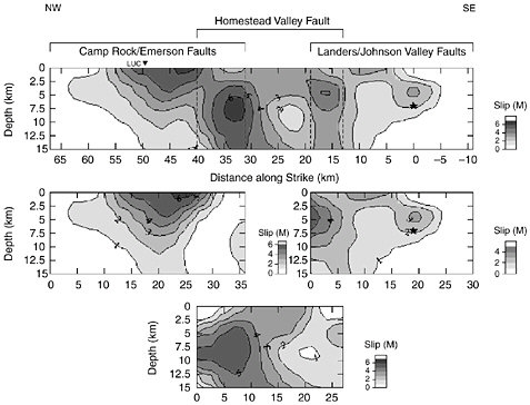
FIGURE 5.7 Slip distribution on three fault segments determined from strong-motion, teleseismic, and geodetic data for the 1992 Landers, California, earthquake. The combined, projected slip summed from the three fault segments is shown above the slip distributions for the individual segments. Note that there is ample slip near segment boundaries and that slip on the ends of the fault terminates within fault segments. SOURCE: D.J. Wald and T.H. Heaton, Spatial and temporal distribution of slip for the 1992 Landers, California earthquake, Bull. Seis. Soc. Am., 84, 668-691, 1994. Copyright Seismological Society of America.
Deep Earthquakes
Earthquakes below 70 kilometers present special research problems because fault ruptures at these depths cannot be explained by brittle fracture or friction (Figure 5.8; see Section 2.5). Although their depths limit the seismic hazard (164), these intermediate- and deep-focus events provide primary constraints on subduction-zone processes. According to plate-tectonic theory, slabs are colder and thus denser and stronger than the surrounding mantle; their sinking involves a balance between the gravitational forces that pull them down and the viscous resistance of the mantle to this penetration (165). The nonhydrostatic stresses engendered within cold slabs during the subduction process appear to be responsible
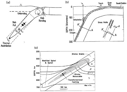
FIGURE 5.8 Conceptual models for earthquakes in descending lithospheric slabs. (a) Generic model for the stresses that cause intraplate earthquakes in slabs. The thermal buoyancy force Fb and its slab-normal and down-dip components, Fn and Fd, are shown for an element of volume. M is the near-trench bending moment. Tc is the critical temperature above which the slabs are too weak to support earthquakes. (b) Some aspects of slab structure that may contribute to earthquake occurrence in the intermediate-focus zone (70 to 300 kilometers), including zones of weakness from prior normal faulting of the oceanic lithosphere, bending stresses in the slab (inset diagram), dehydration-embrittlement, and the densification during the gabbro-to-eclogite phase transition. (c) Physical state of the deep-focus zone (300 to 700 kilometers) showing the equilibrium boundaries of the a, ß, and ? phases of olivine and the phase transition of g-olivine to magnesiowüstite (Mw) and perovskite (Pv) (solid and dashed lines) and the region where a-olivine may be metastable (stippled region). According to one hypothesis, deep-focus earthquakes occur by transformational faulting inside the metastable wedge. SOURCE: Modified from S.H. Kirby, Intraslab earthquakes and phase-changes in subducting lithosphere, Rev. Geophys. Suppl., 33, 287-297, 1995. Copyright 1995 American Geophysical Union. Reproduced by permission of American Geophysical Union.
for all intermediate- and deep-focus earthquakes, and the distribution of stresses implied by this model explains the general pattern of focal mechanisms, which are observed to shift from down-dip tension to down-dip compression with increasing depth (166).
Compared to shallow-focus ruptures, large deep-focus earthquakes have relatively few aftershocks; however, they show similar slip mechanisms, stress drops, source durations, and b values, and they have similar rupture complexity (167). The frequency of earthquakes in subduction zones decreases exponentially with depth, reaching a minimum near 350 kilometers, then increases to a maximum near 600 kilometers before falling rapidly to zero at depths below about 670 kilometers (168). The bimodal distribution of subduction-zone seismicity could be due to a minimum in stress at 300 kilometers or to a change in mechanism. The seismicity cutoff coincides closely with a sharp discontinuity in seismic structure attributed to mineralogical phase transitions.
The principal unanswered questions concern the mechanisms for initiating and sustaining shear instabilities for shear failure of rocks at high pressure and temperature in the descending lithosphere (169). The mechanisms that have received serious consideration include plastic and melting instabilities (170), embrittlement caused by dehydration reactions (171), and instabilities associated with recrystallization during polymorphic phase transitions (172). Dehydration embrittlement, which involves the lowering of the effective normal stress by water pressure from dehydration, is a leading contender for at least some intermediate-focus events (173), while transformational faulting initiated by the olivine-spinel phase reaction in metastable parts of the descending slab is favored by many for deep-focus events (174). The mechanism for the latter involves lenses of the high-pressure phase, or “anticracks,” that act as compressional analogues of the tensile microcracks in enabling macroscopic brittle shear failure (175). Like tensile cracks, the anticracks have no shear strength since the ultrafine-grained high-pressure phase flows superplastically. Moreover, shear localization is enhanced by heat released during exothermic phase transitions (176).
In 1994, deployments of portable arrays recorded valuable near-source data for two of the largest deep-focus earthquakes of this century (177), raising serious questions for all of the rupture models based on laboratory experiments. Specifically, rupture during these two events traversed a wide range of mantle temperatures, contrary to the controlled conditions of pressure and temperature in laboratory experiments (178). It is likely that there was widespread melting on the fault plane during the Bolivian earthquake, raising the possibility that shear heating may play a key role (179). Important questions about this mechanism include whether melting is important to the nucleation of earthquakes or becomes
important only when the rupture is established and propagating. In summary, models for deep- and intermediate-focus earthquakes are still quite general and qualitative compared to the detailed understanding of rupture near the surface.
Key Questions
-
What is the magnitude of the stress needed to initiate fault rupture? Are crustal faults brittle in the sense that ruptures require high stress concentrations or local weak spots (low effective normal stress) to nucleate but, once started, large ruptures reduce the stress to low residual levels?
-
How do earthquakes nucleate? What is the role of foreshocks in this process? What features characterize the early post-instability phase?
-
What is the nature of fault friction under slip speeds characteristic of large earthquake ruptures? How can data on fault friction from laboratory experiments be reconciled with the earthquake energy budget observed from seismic radiation and near-fault heat flow?
-
How much inelastic work is done outside a highly localized fault-zone core during rupture? Is the porosity of the fault zone increased by rock damage due to the passage of the rupture-tip stress concentration? What is the role of aqueous fluids in dynamic weakening and slip stabilization?
-
Do minor faults bordering a main fault become involved in producing unsteady rupture propagation and, potentially, in arresting the rupture? Is rupture branching an important process in controlling earthquake size and dynamic complexity?
-
Are strong, local variations in normal stress generated by rapid sliding on nonplanar surfaces or material contrasts across these surfaces? If so, how do they affect the energy balance during rupture?
-
What produces the slip heterogeneity observed in the analysis of near-field strong-motion data? Does it arise from variations in mechanical properties (quenched heterogeneity) or stress fluctuations left in the wake of prior events (dynamic heterogeneity) or both in concert?
-
Under what conditions will ruptures jump damaged zones between major fault strands? Why do many ruptures terminate at releasing stepovers? How does the current state of stress along a fault segment affect the likelihood of ruptures cascading from one segment to the next?
-
What are physical mechanisms for the near-field and far-field dynamical triggering of seismicity by large earthquakes?
-
What are the sources of short apparent slip duration?
-
How short can the rise time be and still be consistent with the observed seismic data? How does the rise time scale with earthquake
-
size? How short will the rise time be for much larger earthquakes in which the slip may exceed 10 meters? Is it limited by the geometry of the fault plane or the dynamics of friction at high slip velocities?
-
What physical mechanisms explain the deep-focus earthquakes that occur in the descending lithosphere down to depths of nearly 700 kilometers? How do these mechanisms differ from shallow seismicity?
5.5 WAVE PROPAGATION
Earthquake damage is caused primarily by seismic waves. Seismic shaking is influenced heavily by the details of how seismic waves propagate through complex geological structures. In particular, strong ground motions can be amplified by trapping mechanisms in sedimentary basins and by wave multipathing along sharp geologic boundaries at basin edges, as well as by amplifications due to near-site properties. Although near-site effects such as liquefaction can be strongly nonlinear, most aspects of seismic-wave propagation are linear phenomena described by well-understood physics. Therefore, if the seismic source can be specified precisely and the wave velocities, density, and intrinsic attenuation are sufficiently well known, it is possible to predict strong motions by a forward calculation.
A conspicuous success of earthquake physics has been the development of computational techniques for describing the propagation of seismic waves. These techniques yield approximate solutions to the forward problem of seismic-wave propagation, which is to predict the wavefield as a function of position and time knowing the source and a model describing the Earth’s elastic and anelastic constitutive properties (180). Such calculations can be used to predict the strong ground motions in the vicinity of an anticipated earthquake. Moreover, they provide the theoretical framework for solving the structural inverse problem (to estimate a set of constitutive parameters from recordings of the wavefield and knowledge of the source), as well as the source inverse problem (to estimate a set of source parameters from recordings of the wavefield and knowledge of the structure). The effects of source excitation and wave propagation are coupled in seismograms, which complicates their separation. Recent progress on solving these coupled inverse problems, outlined in the previous chapter, has enhanced the predictive capabilities of wavefield modeling. At present, numerical simulations using good propagation models can reproduce the recorded waveforms of low-frequency motions (less than 0.5 hertz) from events such as the 1994 Northridge earthquake and match the spectral amplitudes at higher frequencies with moderate success (181). However, matching the waveforms at higher fre-
quencies will require much better seismological imaging of both the rupture process and the crustal structure.
For engineering applications, a high-priority goal is to determine the structure of high-risk, urbanized areas of the United States well enough to predict deterministically the surface motions from a specified seismic source at all frequencies up to at least 1 hertz and to formulate useful, consistent, stochastic representations of surface motions up to at least 10 hertz.
Theory and Numerical Methods
The Earth is almost spherical, and its internal layering is nearly concentric, at least on the gross scales of the mantle and core. Seismological research during the first 40 years of the twentieth century established the basic features in the radial distribution of seismic velocities and density, culminating in the Jeffreys-Bullen model. More recent work has refined these spherically symmetric global models, particularly with regard to the structure of the upper-mantle and midmantle transition zone (182), and has provided a number of regionalized estimates of the layering of the crust and upper mantle beneath both continents and oceans (183). For such one-dimensional Earth models, the partial differential equations of elastodynamics can be simplified to a set of ordinary differential equations, which can be solved numerically using various methods.
In the lowest frequency bands (0.0003 to 0.1 hertz), the most general and accurate techniques involve the representation of the displacement field in terms of the normal modes of the elastic structure (184). For compact seismic sources, theoretical seismograms synthesized from good one-dimensional Earth models by normal-mode summation can show remarkable agreement with observed seismograms. The normal-mode representation forms the basis for recovering earthquake source parameters from surface-wave and other low-frequency data. For three-dimensional Earth models where the deviations from spherical symmetry are relatively small, normal-mode perturbation theory provides general and efficient methods for computing theoretical seismograms, and it has been applied in many global tomographic studies to invert low-frequency seismic waveforms for three-dimensional Earth structure.
At high frequencies, the calculations become more difficult, and methods that approximate the waves as energy packets traveling along discrete ray paths are often employed (185). Ray theory is usually less accurate, but it provides an adequate representation of many seismic phases, especially the first arrivals at teleseismic distances, and it has been used extensively in algorithms for recovering source parameters from seismic waveforms. It is also the preferred representation in tomographic studies
that image three-dimensional Earth structure from measurements of body-wave travel times.
The strongest ground motions during an earthquake are often generated by the trapping of waves within sedimentary basins and other three-dimensional structures (e.g., effects in Mexico City from the distant 1985 Michoacan earthquake), or by interference among elastic waves that have been diffracted along different paths at the edges of such structures (e.g., 1995 Hyogo-ken Nanbu earthquake). The semianalytical methods described above are often too inaccurate to describe the complexities observed in real seismograms in such cases, and seismologists have resorted to solving numerically the equations of motion for models discretized on two-dimensional and three-dimensional grids using finite-difference (186), finite-element (187), and pseudospectral techniques (188).
Crustal Waveguide Effects
As seismic waves propagate away from the fault, their intensity is reduced by geometrical spreading. For body waves in a uniform material, geometrical spreading reduces the amplitude in inverse proportion to distance (r–1). For surface waves, the factor is r–1/2. In a layered medium, the effects of spreading are complicated by scattering and internal reflections. When energy is reflected or scattered, it causes the energy to attenuate more than r–1 or r–1/2 (189). However, internal reflections can also in result in enhanced ground motions at large distances from the hypocenter (190).
The advent of broadband seismometers in the late 1980s provided a vastly improved representation of actual ground motions against which to test wave propagation models. One such test, shown in Figure 5.9, demonstrates the ability of wave propagation models to reproduce the various body-wave and surface-wave phases recorded at a distance of about 160 kilometers from a small earthquake. The critical reflections from the Moho (SmS phases) that dominate the seismograms shown in Figure 5.9 have an important effect on the attenuation of strong ground motion from earthquakes. The arrival of these critical reflections, beginning at a distance of about 50 kilometers, causes a reduction in the rate of attenuation of ground motion out to distances of about 150 kilometers (Figure 5.10). Although the elevated ground-motion amplitudes in this distance range are usually not large enough by themselves to cause damage, they may produce damage if combined with the amplifying effects of soft soils. The destructive potential of these effects was demonstrated dramatically in the 1989 Loma Prieta earthquake (191) in which major damage was done to buildings and bridges in the San Francisco Bay area located 80 to 90 kilometers from the earthquake.
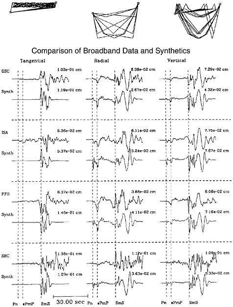
FIGURE 5.9Top: Radial component paths of upgoing, downgoing, and surface-reflected downgoing rays. Bottom: Comparison of recorded and synthetic broadband displacement seismograms of the 1991 Sierra Madre earthquake. SOURCE: Modified from D. Helmberger, D. Dreger, R. Stead, and H. Kanamori, Impact of broadband seismology on the understanding of strong motions, Bull. Seis. Soc. Am., 83, 830-850, 1993. Copyright Seismological Society of America.
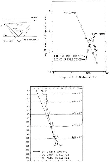
FIGURE 5.10 Effect of crustal structure on ground motion attenuation. Synthetic seismograms (bottom) calculated for a crustal waveguide (top left). The contributions of direct and reflected rays (top right) to the attenuation relation are shown in the top right panel. SOURCE: R.W. Burger, P.G. Somerville, J.S. Barker, R.B. Herrmann, and D.V. Helmberger, The effect of crustal structure on strong ground motion attenuation relations in eastern North America, Bull. Seis. Soc. Am., 77, 420-439, 1987. Copyright Seismological Society of America.
At larger distances (100 to 1000 kilometers), the effect of the crustal waveguide becomes increasing complex, and shear-wave arrivals are composed mainly of multiple reflections of S waves between the Moho and the surface (the Lg phase). This phenomenon is illustrated in the body-wave seismogram of the 1988 Saguenay earthquake recorded at a distance of 600 kilometers at Harvard, the first broadband recording of a moderate-magnitude earthquake in eastern North America (Figure 5.11). The synthetic seismograms calculated using a simple point source time function and a one-dimensional velocity model for the region provide a remarkably close fit to both the long-period and the short-period components of the Pnl and Snl body-wave phases generated by the crustal waveguide.
Effects of Sedimentary Basins
For many years, it has been known that ground motions on soil sites are typically stronger than those on rock sites due to the low shear moduli of the near-surface (upper 30 meters) sedimentary units (192). While this local effect has been recognized by engineers and incorporated into build
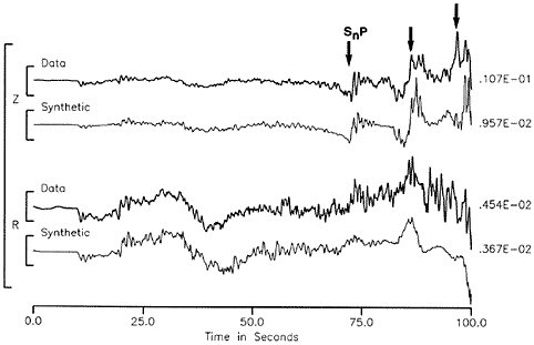
FIGURE 5.11 Comparison of recorded and synthetic broadband displacement seismograms of the 1988 Saguenay earthquake recorded at Harvard. SOURCE: C.K. Saikia, Modified frequency-wavenumber algorithm for regional seismograms using Filon’s quadrature: Modeling of Lg waves in eastern North America, Geophys. J. Int., 118, 142-158, 1994. Reproduced by permission of Blackwell Publishing.
ing codes, recent observations and theoretical studies have demonstrated that a variety of complex wave propagation effects can also influence the ground motions on soil sites that are located in sedimentary basins. In many cases, the impact of the deeper basin structure is much greater than that due to the surficial site materials.
Seismic body waves entering a basin through its thickening edge can become trapped within the basin if postcritical incidence angles develop, generating surface waves whose amplitude and duration are significantly larger than those of the incoming body waves. This phenomenon is illustrated in Figure 5.12, which shows strong-motion velocity time histories of the 1994 Northridge earthquake recorded on a profile of stations, it begins in the San Fernando Valley, crosses the Santa Monica Mountains, and extends into the Los Angeles basin. The ground motions recorded on rock sites in the Santa Monica Mountains are brief and are dominated by the direct body waves. In contrast, the time histories recorded in the Los Angeles basin have long durations, and their peak velocities are associated not with the direct body waves but with surface waves generated at the northern edge of the Los Angeles basin. The ground motions were further amplified as they crossed the Santa Monica fault, which marks an abrupt deepening of the Los Angeles basin. This amplification is reflected dramatically in the damage distribution indicated by red-tagged buildings, which are concentrated immediately south of the fault scarp. The strong correlation of the damage pattern with the fault location indicates that the underlying basin-edge geology, not shallow soil conditions, is controlling the ground-motion response. The large amplification results from constructive interference of direct waves with the basin-edge generated surface waves. As described in Chapter 2, the 1995 Hyogo-ken Nanbu earthquake provided dramatic evidence for the destructive potential of basin-edge effects (193), manifested as severe damage in a narrow zone running parallel to the causative faults through Kobe and adjacent cities (Figure 2.22). These and other simulations of basin waves (194) demonstrate that it is now possible to perform simulations of strong ground motions in basin structures, and these demonstrations form the basis for the simulation of ground motions from scenarios of future earthquakes (195).
Wave propagation in fluid-saturated sediments can exhibit special complexities that cannot be modeled in terms of a single elastic continuum. Early work by Maurice Biot and recent research shows that a fluid-saturated porous solid can support two P waves as well as one S wave. The surface waves on such a medium have not been adequately studied. This is an important subject in which more research is necessary in terms of constitutive relations and boundary conditions (196).
Rupture Propagation Effects
During an earthquake, seismic waves are emitted from the slipping part of the fault behind the rupture front. Since the rupture velocity is usually close to the shear-wave velocity, the amplitude of the seismic waves ahead of the rupture front grows progressively as more energy is added by the propagating fault. This energy buildup results in a large pulse of motion at the arrival time of each kind of seismic wave in the seismogram that contains the cumulative effect of rupture on the fault (197). The radiation pattern of the shear dislocation causes the motions of the large pulse to be oriented perpendicular to the fault. Forward rupture directivity effects require two conditions: the rupture front propagates toward the site, and the slip direction is aligned with the site. These conditions are readily met at locations away from the epicenter in strike-slip faulting and are also met during dip-slip faulting in the region located updip of the hypocenter. The enormous destructive potential of near-fault ground motions was manifested in the 1994 Northridge and 1995 Hyogoken Nanbu earthquakes. In each of these earthquakes, peak ground velocities as high as 175 centimeters per second were recorded (Figure 5.13). The periods of the near-fault pulses recorded in both of these earthquakes were in the range of 1 to 2 seconds, comparable to the natural periods of structures such as bridges and midrise buildings, many of which were severely damaged. These near-fault recordings have led to revisions of building codes in the United States.
Anelastic Attenuation Effects
The effects of absorption are described by the quality factor Q, which is inversely proportional to the fractional loss of energy per wave cycle. In the Earth, the Q value depends on the frequency of the seismic wave and the properties of the rocks. Values of Q in the crust and lithosphere are much lower than those in the underlying mantle, and they vary significantly with the tectonic environment. In general, attenuation is lower in tectonically stable regions, so earthquakes cause damage at much greater distances in stable regions than in tectonically active regions. Also the frequency dependence of Q is greater in areas of active tectonics (198). Proposed absorption mechanisms in the crust include frictional sliding on cracks, thermoelastic effects, grain boundary deformation, and dissipation by fluid movement within cracks and pores. For depths less than 1 kilometer, there can be strong attenuation from open cracks in near-surface rocks and losses in unconsolidated soils, causing the intensity of ground motions to diminish with increasing frequency beyond about 5
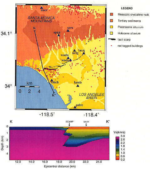
hertz. The distribution of Q for sedimentary rocks in basins influences the duration of shaking from strong earthquakes.
Nonlinear Site Effects
Soil response to strong shaking is a complex, nonlinear phenomenon that has long been investigated in laboratory experiments and in the field following large earthquakes (199). Laboratory tests clearly demonstrate nonlinear strain behavior in soils under dynamic loading. This nonlinearity is manifested by a reduction in shear modulus and an increase in
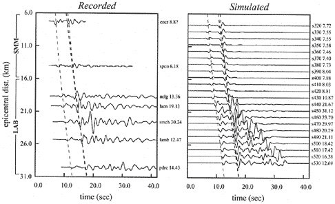
FIGURE 5.12 Basin effects in Santa Monica from the 1994 Northridge earthquake. Upper left panel is a geological map with the locations of seismic stations (triangles) and the scarp of the Santa Monica fault (arcuate black lines). Lower left panel is a sheer velocity model of the upper crust along map profile kk’. Upper panels compare the observed seismograms (left) with seismograms simulated from the model (right). The simulation indicates that the large pulse at station smch is caused by the focusing at the rock-sediment interface along the Santa Monica fault. SOURCE: Modified from R.W. Graves, A. Pitarka, and P.G. Somerville, Ground motion amplification in the Santa Monica area: Effects of shallow basin edge structure, Bull. Seis. Soc. Am., 88, 1224-1242, 1998. Copyright Seismological Society of America.
damping as shear strain levels increase beyond about 10–4 to 10–5 or as ground acceleration becomes greater than about 0.1g. This softening causes the fundamental period of the soil layer to lengthen. At higher frequencies, cyclic pore pressure increases may produce cyclic strain hardening, which is manifested by high-frequency spikes toward the end of the record, increasing the duration of the record and sometimes producing the largest accelerations. These effects have been demonstrated in the small number of data sets where surface and subsurface seismic data are available (200) to enable direct comparison between the motion in the rock or stiff soil (which is assumed to be linear) and the resulting motion
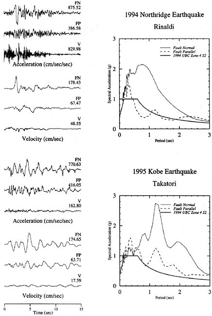
FIGURE 5.13 Recorded near-fault acceleration and velocity time histories and acceleration response spectra of the 1994 Northridge earthquake (top) and 1995 Hyogo-ken Nanbu earthquake (bottom), showing pulse-like motion on the strike-normal component of motion, which is much larger than the strike-parallel component at periods longer than about 0.4 second. SOURCE: P. Somerville, URS Corporation.
in the overlying softer soil. If nonlinear effects are important, then strong ground motions for large earthquakes can be difficult to predict from the measured accelerations during smaller events. Another complicating factor is that cohesionless soils are also subject to liquefaction and lateral spreading due to pore pressure effects (201). Nevertheless, numerical codes that account for soil nonlinearity are numerous, ranging from equivalent linear models to fully nonlinear models that also incorporate pore-pressure generation (202).
High-Frequency Ground Motions
Ground motions at frequencies above 1 hertz are the most damaging motions for small- and moderate-sized structures, and they also contain important information about the seismic source and details of stress on the fault plane. The character of high-frequency ground motions was documented from the analysis of the first strong-motion accelerograms (203). A key parameter is the corner frequency, which scales as the inverse of the rupture duration for events recorded in the far field or to the slip duration at a location on the fault for large events recorded by nearby seismometers. At low frequency, the displacement amplitude spectrum is constant with increasing frequency up to the corner frequency, where it changes slope and rolls off as the square of frequency (204). Correspondingly, the acceleration amplitude spectrum increases with frequency squared below the corner frequency and becomes flat above the corner frequency. Above 5 to 10 hertz, the acceleration spectrum declines rapidly with increasing frequency beyond a transition value denoted by fmax (205). Many theoretical studies have attempted to explain the flat portion of the acceleration spectrum (206). The spatial coherence of ground motions decreases rapidly with increasing frequency (207). Although the cause of this incoherence is not well understood, it may be due in part to focusing effects caused by irregular bedrock topography (208).
Key Questions
-
How are the major variations in seismic-wave speeds related to geologic structures? How are these structures best parameterized for the purposes of wavefield modeling?
-
What are the contrasts in shear-wave speed across major faults? Are the implied variations in shear modulus significant for dynamic rupture modeling? Do these contrasts extend into the lower crust and upper mantle?
-
How are variations in the attenuation parameters related to wave speed heterogeneities? Is there a significant dependence of the attenua-
-
tion parameters on crustal composition or on frequency? How much of the apparent attenuation is due to scattering?
-
What are the differences in near-fault ground motions from reverse, strike-slip, and normal faulting? In thrust faulting, how does energy trapped between the fault plane and free surface of the hanging-wall block amplify strong ground motions?
-
How does the structure of sedimentary basins affect the amplitude and duration of ground shaking? How much of the amplification pattern in a basin is dependent on the location of the earthquake source? Can the structure of sedimentary basins be determined in sufficient detail to usefully predict the pattern of ground shaking for future large earthquakes?
-
Are fault-parallel, low-velocity waveguides deep-seated features of faults? How continuous are they along strike and dip? Can studies of fault-zone trapped waves constrain the effective rheological parameters of the fault zone, such as effective fracture energy?
-
Is the ability to model recorded seismograms limited mainly by heterogeneity in source excitation, focusing by geologic structure, or wavefield scattering?
-
What role do small (sub-grid-scale) heterogeneities and irregular interfaces play in wave propagation at high frequencies? How do they depend on depth, geological formation, and tectonic structure? How important is multiple scattering in the low-velocity, uppermost layers? Can stochastic parameterizations be used to improve wavefield predictions?
5.6 SEISMIC HAZARD ANALYSIS
Although earthquakes cannot be predicted in the short term with any useful accuracy and generality and the feasibility of intermediate-term prediction is still an open question, the magnitudes and locations of larger events can be forecast over the long term, and their effects can be anticipated. Seismic hazard analysis (SHA), described in Chapter 3, involves the characterization of potential earthquake activity and associated ground motions in a form, either probabilistic or scenario based, that is useful for seismic design and emergency management. The scientific basis for probabilistic seismic hazard analysis (PSHA) is currently being improved by (1) the addition of denser and more precise geodetic and geologic data sets to seismic hazard characterization and (2) a better understanding of the geological controls on strong ground motions. The challenge is to recast the methodology of seismic hazard analysis in a way that more explicitly accounts for the dependence of earthquake phenomena on time.
Earthquake Forecasting
Historically, most seismic hazard analyses have assumed that earthquakes can be described as a Poisson process, for which the probability of at least one earthquake in a given time t is
P(t) = 1 – e–rt,
(5.3)
where the rate parameter r can be estimated from the historical or prehistoric rate of earthquakes (e.g., a plot of magnitude versus frequency determined from seismic monitoring or paleoseismology). For a simple Poisson process, the probability per unit time is independent of absolute time and the time elapsed since the last event. These properties make the problem of earthquake forecasting a fairly straightforward exercise. For example, in the preparation of the recent USGS maps, probabilities were calculated with a Poisson model once the magnitude-frequency relation had been established for each of the seismic sources.
Driven by the development of plate tectonics, a growing catalog from seismic monitoring, and increasingly detailed measurements of historical seismic activity and fault slip, there is growing interest in time-dependent forecasting techniques for specific earthquakes. This work originated from the early models of earthquake recurrence that linked spatial and temporal aspects of seismicity with rates and pattern of fault slip. A simple time-dependent probabilistic model of the occurrence of large earthquakes has occasionally been implemented in PSHA in cases where the historical or paleoseismic record supports it. Compared to the Poisson formulation, the most important feature of this model is that the probability of occurrence of a similar event increases with time since the last one.
The challenge has been to identify data sets and develop physical models that might explain such time-dependent features of earthquake recurrence. Currently, these efforts are advancing on several fronts, some of which take very different tacks (e.g., seismic gaps versus earthquake clustering). Such differences may lead to discrepant forecasts. These points are illustrated below in discussions of characteristic earthquakes, seismic gaps, moment-rate budgeting, clustering, and stress-transfer effects.
Characteristic Earthquakes The characteristic earthquake hypothesis states that seismic moment release on an individual fault segment is dominated by a characteristic earthquake rupturing the entire length of the segment (i.e., the largest possible earthquake for that segment), and that moderate earthquakes within one magnitude range below the characteristic event may be rare or entirely absent. The model implicitly assumes that (1) rupture is limited to geometrically defined fault segments, (2) the displacement per event is constant at a point, (3) the slip rate along
the fault is variable, and (4) slip deficits at the ends of fault are not “filled in” by slip from smaller earthquakes.
From the perspective of hazard assessments, this hypothesis offers tremendous simplification because only one earthquake scenario is considered (the characteristic earthquake) for each fault segment. Moreover, the size of this earthquake can be estimated from the length of the fault segment and moment-length scaling relations. In this way, the hypothesis reduces the dimension of the earthquake forecasting problem to one in which time is the only independent variable. Because of these simplifications, characteristic earthquakes have been incorporated into a large number of seismic hazards analyses (209).
Seismic Gap Hypothesis Building on the characteristic earthquake hypothesis, the seismic gap hypothesis addresses the distribution of these large events through time. To estimate earthquake likelihood for use in seismic hazard studies, the seismic gap model is implemented as follows. Mapped faults are divided into segments, and a characteristic magnitude is estimated for each segment. The slip rate on the fault is estimated from the displacement and age of features offset by the fault, and the characteristic slip is estimated from historical slip data or from regression relationships on magnitude and slip. The mean recurrence time is estimated from either the times of known earthquakes on the segment or the ratio of characteristic slip to fault slip rate. The probability distribution of recurrence times is estimated, and the conditional probability of an earthquake during some time interval is computed. The critical question to address is whether forecasted earthquakes in seismic gaps occur with greater probability than a simple random occurrence.
Moment-Rate Budgeting One approach to forecasting future earthquakes is to balance the long-term rates of fault slip and moment release as inferred from seismic monitoring. In practice, the application of moment-rate budgeting is difficult because the results are sensitive to the completeness of the historical catalog and the past distribution of earthquakes in space and time. Key, but controversial, assumptions of this method are that the long-term slip rates are representative of present rates and that the slip rates are completely seismogenic. The latter assumption may hold for crustal earthquakes, but it does not appear to be valid for many subduction zones, where significant aseismic deformation is occurring.
Clustering The term clustering is commonly used to describe concentrations of earthquakes in space, time, or both. Earthquakes are much more frequent in some places than in others, even along major faults or
plate boundaries, as seen from inspection of maps of earthquake locations. The most abundant (and obvious) example of earthquake clustering in time and space is the occurrence of aftershocks (see Chapter 4). Indeed, many complete catalogs of earthquakes are dominated by aftershocks of moderate to large events (210). Thus, the occurrence of a single earthquake greatly increases the probability of another event in the same location.
Although the physical origin of clustering behavior is not clear, it has important implications for models of earthquake occurrence. Clustering suggests a causality between earthquakes that could change many of the assumptions that underlie seismic hazard assessments. In short to intermediate time scales, the most dangerous regions may be those that have recently experienced large earthquakes, rather than the locked portions of seismically active faults.
Stress Interactions Identifying the origins of clustering, or distinguishing among different models of earthquake recurrence, will require an explicit physical theory of seismic activity. Important components of such a theory will include an explicit model for stress evolution on major faults due to tectonic stress accumulation, previous earthquakes, and inelastic stress relaxation as well as the evolution of frictional strength on faults, the mechanical strength of materials off the fault, and the rupture of virgin rock required to accomplish finite displacements in a brittle medium. Such a complete theory will be difficult to develop and difficult to confirm experimentally because it requires a long span of accurate earthquake information including focal mechanisms. Furthermore, the stress model must include tectonic stress accumulation, for which there is no definitive model at present. However, significant progress has been made on parts of the theory.
An important first step was the development of expressions to calculate stresses everywhere in a homogeneous elastic half-space due to an arbitrary dislocation (211). These expressions allow calculations of the change in stress across any existing fault due to earthquakes causing known displacements. With this model, it has become routine to calculate stress changes for all earthquakes above M 5 in populated regions. Using these methods to calculate tectonic stress accumulations is more complex because it requires assumptions about strain partitioning throughout fault and plate boundary zones.
Application to Seismic Hazard Analysis There have been continuing efforts to utilize the understanding of earthquake forecasting to improve the capabilities of PSHA. To this end, the recent USGS ground-motion mapping study incorporated characteristic earthquakes for a
limited number of fault segments. Other hazard analyses have also incorporated time-dependent probabilities (212). Time-dependent seismic hazard maps have been produced for California by the Southern California Earthquake Center and the California Division of Mines and Geology (CDMG) (213). The CDMG maps show substantial differences from the time-independent maps for certain faults.
Several efforts are also under way to produce urban seismic hazard maps that merge probabilistic seismic hazard assessment with site response and, in some cases, three-dimensional basin effects and rupture directivity. These maps, at scales of 1:24,000 to 1:50,000, could be used for engineering design purposes, loss estimation, and land-use planning.
Prediction of Strong Ground Motions
Seismic waves travel through a medium having a free surface, strong variations (usually increases) of seismic velocity with depth, large-scale lateral variations in seismic velocities related to mountains and sedimentary basins, small-scale lateral variations (scatterers), and dramatically different elastic properties at individual observation sites (local soil conditions). The wave trains generated by even very simple sources, such as explosions, can become highly complex due to propagation through such heterogeneous media. Source effects such as rupture directivity further add to the spatial variation of ground motions (see Section 5.5).
This large degree of variability in ground-motion characteristics presents a formidable challenge to earthquake engineers and engineering seismologists whose role is to characterize ground motions for the seismic design of structures. During the past two decades, careful studies of ground motions from well-recorded earthquakes, the application of rigorous representations of earthquake sources as shear dislocations, and the use of increasingly realistic methods of modeling seismic wave propagation through heterogeneous structures have resulted in a greatly enhanced ability to understand and predict the complex waveforms of strong ground-motion recordings. Common methods to estimate ground motions are summarized below.
Empirical Engineering Models of Strong Ground-Motion Attenuation A convenient collection of recent empirical ground-motion models was published in the 1997 January-February issue of Seismological Research Letters (214). These ground-motion models are for distinct tectonic categories of earthquakes: shallow crustal earthquakes in tectonically active regions, shallow crustal earthquakes in tectonically stable regions, and subduction-zone earthquakes. Subduction-zone earthquakes are further subdivided into those that occur on the shallow plate interface and those
that occur at greater depths within the subducting plate. Significant differences exist in the ground-motion characteristics among these different earthquake categories, as illustrated in Figure 5.14.
The process of developing modern empirical ground-motion attenuation relations has become a routine endeavor. First, a comprehensive set of strong-motion data is compiled in which the following quantities are rigorously quantified or classified: earthquake category (e.g., crustal or subduction), seismic moment and moment magnitude, focal mechanism, geometry of the earthquake’s rupture plane and distance of each recording station from this plane, and recording site conditions. Next, a complex functional form is usually selected and fit to the data. The equations that are developed relate ground-motion parameters (such as peak ground acceleration, response spectral acceleration, strong-motion duration) to the source parameters of magnitude and mechanism, the path parameters (usually source-to-site distance and sometimes focal depth), and local parameters (site geology and sometimes depth to basement rock).
Specification of Uncertainty in Ground-Motion Attenuation Models and SHA The complete description of a ground-motion parameter includes the central estimate of the parameter and its variability. The standard error in the predicted ground-motion level is relatively high; typically the median plus one standard deviation level of ground motion is about a factor of 1.5 to 2 greater than the median value (215).
Seismic hazard calculations for critical facilities include a comprehensive representation of uncertainty commonly separated into epistemic and aleatory components (216). Epistemic uncertainty is due to incomplete knowledge and data and, in principle, can be reduced by the collection of additional information. Aleatory uncertainty is due to the inherently unpredictable nature of future events and cannot be reduced. The total uncertainty is obtained from the combination of the epistemic and aleatory components. The epistemic uncertainty is usually represented by alternative branches on a logic tree, leading to alternative hazard curves. These alternative hazard curves can be used to define hazard curves at different confidence levels. Each hazard curve is produced from an integration over the aleatory component.
Characterization of Site Response Local geological conditions have a primary influence on the amplitude and frequency content of strong ground motions. In particular, the vertical gradient in shear-wave velocity (which generally increases rapidly with depth just below the surface) gives rise to motion amplification due to impedance contrast effects, which may be offset by the effects of viscoelastic damping and nonlinear response of the medium. The simplest way to account for effects of local
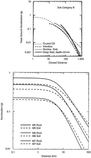
FIGURE 5.14 (Top) Peak acceleration attenuation relations for soil sites for M 6.5 earthquakes for a range of tectonic categories of earthquakes. SOURCE: P. Somerville, URS Corporation. (Bottom) Peak acceleration attenuation relations for crustal earthquakes showing the dependence on magnitude and site category. SOURCE: N.A. Abrahamson and K.M. Shedlock, Overview of ground-motion attenuation models, Seis. Res. Lett., 68, 9-23, 1997. Copyright Seismological Society of America.
geological conditions is to use empirical ground-motion attenuation relations for the site geology category (e.g., alluvium, rock) that are representative of the site. However, the response at a given site belonging to a broad category (e.g., “soil,” “rock”) is in general different from the average response of a large number of sites belonging to that category. Furthermore, the variability of the response between these many sites will, in general, be larger than the variability in response of a single site due to multiple earthquakes.
Another common procedure to estimate site response is with physically based models of vertical shear-wave propagation through a horizontally layered soil column whose properties, including shear-wave velocity, material damping, and density, have been determined from field and laboratory measurements. Some models include the nonlinear response of soils, which can have an important influence on the amplitude and frequency content of the ground motion. The important effect of nonlinear soil behavior on site response has been incorporated in the site response factors that are embodied in current building codes and provisions (217). In these codes and provisions, site response is represented by period- and amplitude-dependent factors derived from sets of recorded data and from analyses of site response based on nonlinear or equivalent-linear models of soil response.
Ground-Motion Prediction Using Seismological Models Based on developments in theoretical and computational seismology and on strong-motion recordings from a large number of major earthquakes that began with the 1979 Imperial Valley earthquake, much progress has been made in understanding the origin and composition of strong ground motion. In many instances, the causes of the large variations in strong ground-motion recordings are now understood. This understanding is being applied to the problem of constructing realistic earthquake scenarios (i.e., predicting ground motions from potential future earthquakes). The simplest seismologically based simulations treat strong motion as a time sequence of band-limited white noise. A Fourier spectral model of the ground motion is constructed, starting with a model of the source spectrum and modifying its shape by factors to represent wave propagation effects (218).
More complex methods have been developed that have a more rigorous basis in theoretical and computational seismology with fewer simplifications than the stochastic model. The earthquake source is represented as a shear dislocation on an extended fault plane, and the wave propagation is rigorously modeled by Green’s functions computed for the seismic velocity structure, which contains the fault and the site, or by empirical Green’s functions derived from strong-motion recordings of earthquakes smaller than the one being simulated. The ground-motion time history is
calculated in the time domain using the elastodynamic representation theorem. This calculation involves integration over the fault surface of the convolution of the slip time function on the fault with the Green’s function for the appropriate depth and distance. For structures having lateral variations in seismic velocities and densities, such as sedimentary basins, wave propagation is modeled numerically using finite difference methods (219).
To simulate broadband time histories using this Green’s function-based approach, ground motions are computed separately in the short-period and long-period ranges and then combined into a single broadband time history. The use of different methods in these two vibrational period ranges is necessitated by the observation that ground motions are much more stochastic at short periods than at long periods. An example of broadband simulation of strong ground motions is shown in Figure 5.15, which compares the recorded and simulated ground motions at Arleta from the 1994 Northridge earthquake.
Because these seismologically based ground-motion models can include the specific source, path, and site conditions of interest, they can be used to generate ground-motion time histories, which augment the recorded data used to generate empirical models. Alternatively, they can be used as site-specific estimates that complement estimates based on empirical models. These seismological models have incorporated important characteristics such as rupture directivity, Moho reflections, and basin effects. Rupture directivity contributed greatly to the generation of peak ground velocities approaching 2 meters per second during the 1994 Northridge, California, and 1995 Kobe, Japan, earthquakes, and approaching 3 meters per second during the 1999 Taiwan event. As a result of these and previous earthquakes, rupture directivity effects have been incorporated in the specification of design ground motions in the 1997 Uniform Building Code and have produced large revisions in the code spectrum, as shown in Figure 5.16.
Key Questions
-
What factors limit fault-rupture propagation? How valid are the characteristic earthquake models? What magnitude distributions are appropriate for different regions?
-
Under what circumstances are large events Poissonian in time? What temporal models and distributions of recurrence intervals pertain to major plate boundary faults? Are these models and distributions different for stable continental regions?
-
Can geodetic (Global Positioning System and interferometric synthetic aperture radar) measurements of deformation be employed to ac-
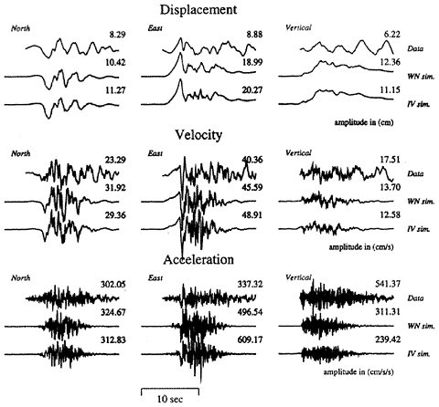
FIGURE 5.15 Comparison of recorded (top row) and simulated (middle and bottom rows) displacement, velocity, and accelerations at Arleta from the 1994 Northridge earthquake, plotted on a common scale with peak value given at the top left corner. SOURCE: P. Somerville, C.K. Saikia, D. Wald, and R. Graves, Implications of the Northridge earthquake for strong ground motions from thrust faults, Bull. Seis. Soc. Am., 86, S115-S125, 1996. Copyright Seismological Society of America.
-
curately constrain short- and long-term seismicity rates for use in seismic hazard assessment? How should geologic and paleoseismic data on faults best be used to determine earthquake recurrence rates?
-
Can physics-based scenario simulations produce more accurate estimates of ground-motion parameters than standard attenuation relationships? Can these simulations be used to reduce the high residual variance in these relationships?
-
What is the nature of near-fault ground motion? How do fault ruptures generate long-period directivity pulses? How do near-fault
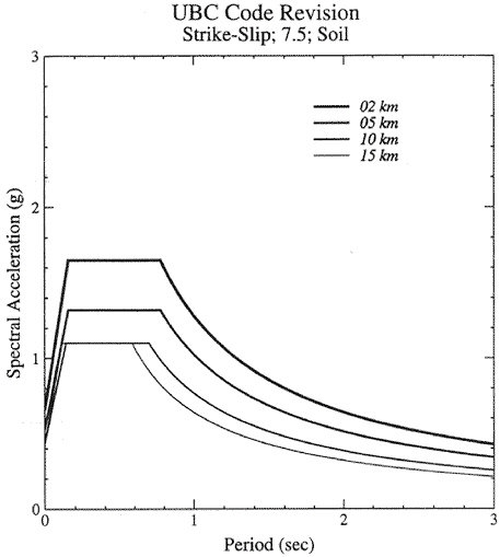
FIGURE 5.16 Design response spectra on soil sites at various distances from a Source Type A fault (maximum M 7.5 or larger) in the 1997 Uniform Building Code (UBC). The 1994 UBC was similar to the spectrum for 15 kilometers’ distance. SOURCE: P.G. Somerville, URS Corporation.
-
ground motions differ between reverse and strike-slip faulting? Can these motions be predicted for scenario earthquakes?
-
What are the earthquake source and strong ground-motion characteristics of large earthquakes (magnitudes greater than 7.5), for which there are few strong-motion recordings? Can the shaking from large earthquakes be predicted accurately from smaller events?
-
How important is the nonlinear seismic response of stable soils in estimating strong ground motion?
NOTES
|
164. |
Earthquakes below crustal depths in descending slabs can shake the surface hard enough to cause deadly secondary effects. For example, the 1970 intermediate-focus Peru earthquake (M 8.0), which occurred at a focal depth of 64 kilometers, initiated the huge Huascarán slide (Figure 3.3) that killed 60,000 people. Seismic waves propagate efficiently below the asthenosphere (i.e., below about 300-kilometer depth) and within the deeper parts of the thickened cratonic lithosphere; the giant M 8.2 deep-focus earthquake 660 kilometers beneath Bolivia was felt by people as far away as Canada. |
|
165. |
M. Vassilou and B. Hager, Subduction zone earthquakes and stress in slabs, Pure Appl. Geophys., 128, 547-624, 1988. |
|
166. |
B. Isacks and P. Molnar, Distribution of stresses in the descending lithosphere from a global survey of focal-mechanism solutions of mantle earthquakes, Rev. Geophys. Space Phys., 9, 103-174, 1971. |
|
167. |
C. Frohlich, The nature of deep focus earthquakes, Ann. Rev. Earth Planet. Sci., 17, 227-254, 1989; H.W. Green, II and H. Houston, The mechanics of deep earthquakes, Ann. Rev. Earth Planet. Sci., 23, 169-213, 1995. |
|
168. |
P.B. Stark and C. Frohlich, Depths of the deepest earthquakes, J. Geophys. Res., 90, 1859-1869, 1985. |
|
169. |
The problem of initiating shear instabilities at very high pressures was broached by D. Griggs and J. Handin (Observations on fracture and a hypothesis of earthquakes, in Rock Deformation, D. Griggs and J. Handin, eds., Geological Society of America Memoir 79, Boulder, Colo., pp. 347-364, 1960). Early experimental and theoretical work focused on the volumetric instabilities in polymorphic phase transitions (e.g., P.W. Bridgman, Polymorphic transitions and geologic phenomena, Am. J. Sci., 243A, 90-97, 1945; F.F. Evison, On the occurrence of volume change at the earthquake source, Bull. Seis. Soc. Am., 57, 9-25, 1967, L. Liu, Phase transformations, earthquakes, and the descending lithosphere, Phys. Earth Planet. Int., 32, 226-240, 1983). The volumetric-instability hypothesis was encouraged by seismological evidence that the great 1970 Columbia deep-focus earthquake radiated energy with a significant isotropic component (A. Dziewonski and J.F. Gilbert, Temporal variation of the seismic moment tensor and the evidence of precursive compression for two deep earthquakes, Nature, 257, 185-188, 1974); however, it is now believed that the isotropic component of deep-focus source mechanisms is small compared to the shear component (D. Russakoff, G. Ekstrom, and J. Tromp, A new analysis of the great 1970 Colombia earthquake and its isotropic component, J. Geophys. Res., 102, 20,423-20,434, 1997). |
|
170. |
D. Griggs, The sinking lithosphere and the focal mechanism of deep earthquakes, in The Nature of the Solid Earth, E.C. Robertson, ed., McGraw-Hill Inc., New York, pp. 361-384, 1972; M. Ogawa, Shear instability in a viscoelastic material as the cause of deep focus earthquakes, J. Geophys. Res., 92, 13,801-13,810, 1987; B.E. Hobbs and A. Ord, Plastic instabilities: Implications for the origin of intermediate and deep focus earthquakes, J. Geophys. Res., 93, 10,521-10,540, 1988. |
|
171. |
C.B. Raleigh, Tectonic implications of serpentinite weakening, Geophys. J. R. Astr. Soc., 14, 113-118, 1967; M.S. Paterson, Experimental Rock Deformation—The Brittle Field, Springer, Berlin, 254 pp., 1978. |
|
172. |
S.H. Kirby, Localized polymorphic phase transitions in high-pressure faults and applications to the physical mechanisms of deep earthquakes, J. Geophys. Res., 93, 13,789-13,800, 1987; C. Meade and R. Jeanloz, Acoustic emissions and shear instabilities during phase transformations in Si and Ge at ultra high pressures, Nature, 339, 616-618, 1989; H.W.I. Green and P.B. Burnley, A new self-organizing mechanism for deep-focus earthquakes, Nature, 341, 733-737, 1989. |
|
173. |
H.W.I. Green and P.B. Burnley, A new self-organizing mechanism for deep-focus earthquakes, Nature, 341, 733-737, 1989; C. Meade and R. Jeanloz, Deep-focus earthquakes |
|
|
ground-motion waveforms, including some produced by source processes such as rupture directivity and others produced by seismic-wave propagation phenomena, such as the trapping of waves in basins, have since been recognized and quantified. |
|
204. |
The f–2 falloff in the displacement amplitude spectrum was recognized in spectra from regional and teleseismic events by K. Aki (Scaling law of seismic spectrum, J. Geophys. Res., 72, 1217-1231, 1967). The low-frequency spectral level is proportional to the seismic moment. Greater stress drops produce a larger high-frequency spectral level for a given seismic moment. It is generally observed that stress drops are approximately uniform over a wide range of earthquake sizes (see Section 2.5). |
|
205. |
It has been shown that the falloff can be explained by attenuation in the near-surface material beneath a site. fmax is observed to correlate with the site geology, with soil sites having lower fmax values than rock sites. The falloff above fmax can be described using a frequency-independent Q. Typically, this is parameterized by k, which is related to the slope of the spectral falloff on a log-linear plot. Although it was initially proposed that fmax is produced by a characteristic length scale of the rupture process, fmax is observed to increase for seismometers located in boreholes, indicating that it is at least in part an artifact of near-surface attenuation. For small earthquakes (M lower than 4), the source corner frequency is often obscured by the effects of near-surface attenuation. |
|
206. |
J.N. Brune (Tectonic stress and the spectra of seismic shear waves from earthquakes, J. Geophys. Res., 75, 4997-5009, 1970) derived this behavior from a earthquake model in which a stress pulse propagated along the fault. He was the first to relate the corner frequency to the radius of rupture and derived the relation between stress drop, seismic moment, and corner frequency. Madariaga (Dynamics of an expanding circular fault, Bull. Seis. Soc. Am., 66, 639-666, 1976) showed that a simple dynamic model of crack nucleation could not produce enough high frequency for an f–2 falloff and suggested that the f–2 falloff was caused by the stopping phase of an earthquake rupture. More recently, the hypothesis that the high-frequency level of the acceleration spectrum is a manifestation of the complexity of the rupture process has been explored. In this view, smaller-scale variations of stress along the fault plane produce higher frequencies of radiated ground motion. Recently, several investigators have proposed fractal models of fault stress heterogeneity. In these models the stress on the fault is a random, self-similar variable with a fluctuation spectrum whose spectral amplitude is proportional to the wavelength raised to some power. Asperities on the fault that produce subevents are described with a power-law distribution of sizes. In separate studies, T. Hanks (b values and ?-? seismic source models; Implications for tectonic stress variations along active crustal fault zones and the estimation of high-frequency strong ground motion, J. Geophys. Res., 84, 2235-2242, 1979), D.J. Andrews (A stochastic fault model, 2. Time-independent case, J. Geophys. Res., 86, 10,821-10,834, 1981), and A. Frankel (High frequency spectral falloff of earthquakes, fractal dimension of complex rupture, b value, and the scaling strength on fault, J. Geophys. Res., 96, 6291-6302, 1991) showed that a flat acceleration spectrum could be explained by a variation of stress drop that was independent of length scale on a fault. Such a scale-independent stress drop is consistent with observations of stress drop being independent of seismic moment. Interestingly, this same variation in stress drop on the fault produced a population of subevents with b values of 1. This b value is similar to those reported for earthquakes in most regions, suggesting that the population statistics of earthquakes may be related to the same stress drop variation responsible for the generation of high-frequency ground motion. |
|
207. |
For example, N.A. Abrahamson, J.F. Schneider, and J.C. Stepp, Empirical coherency functions for applications to soil-structure interaction, Earthquake Spectra, 7, 1-27, 1992; M.I. Todorovska and M.D. Trifunac, Amplitudes, polarity and time of peaks of strong ground motion during the 1994 Northridge, California, earthquake, Soil Dyn. Earthquake Engr., 16, 235-258, 1997; P. Bodin, S.K. Singh, M. Santoyo, and J. Gomberg, Dynamic defor- |


