
3
Formation of Structures and Transients
Solar system and astrophysical plasmas exhibit dynamic behavior whenever different plasma regimes interact with one another. Cosmic plasmas from diverse sources generally populate uniquely defined volumes of space that border against similar volumes populated by plasmas from other sources. Such cosmic plasmas are generally magnetized, and so different plasma regimes resist interpenetration. Examples of plasma regime interactions that occur in the solar system are (1) interactions between coronal mass ejections and the background solar wind, (2) interactions between the solar wind and the ionospheres and magnetospheres of planets, (3) interactions between the corotating, subsonic planetary magnetospheric plasmas and the small magnetospheres surrounding planetary satellites (e.g., the interaction of Ganymede with the magnetospheric plasma of Jupiter), and (4) interactions between the solar wind and the local interstellar medium at the outer reaches of the solar system. As is discussed here, such examples have clear relevance and application to many extrasolar astrophysical plasma systems.
When the relative velocity between plasma regimes is supersonic, the first interaction boundary is a collisionless shock. Whether or not the interaction is supersonic or subsonic, current sheets generally separate the different plasma regimes. The stresses imposed by the interactions also engender the formation of current sheets within the plasma regimes, leading to a cellular structure. Such internal and boundary current sheets imply the existence of high concentrations of energy density and shear stress, and the system responds to dissipate and redistribute the energy and the stress, for example, through magnetic reconnection. These redistributions engender structuring within current sheets, with features such as magnetic flux ropes. The energy redistribution and structuring are accomplished in part by a fundamental property of plasmas, cross-scale coupling. This coupling connects small scales, where particle kinetic effects are important, to large scales, creating features like boundary layers at the walls of cells. Dissipation of kinetic-scale structures can yield charged particle heating and particle acceleration. A special case of cross-scale coupling is hydromagnetic turbulence, which results in the generation of numerous and hierarchically ordered spatial and temporal scales and in the transfer of energy to smaller and smaller spatial scales. The sections that follow discuss each of these structures in turn and identify some of the outstanding questions associated with them. The chapter concludes with a discussion of their universality.
COLLISIONLESS SHOCKS
In an ordinary gas, a shock wave is created in front of an object that is moving at a supersonic velocity (i.e., at a speed with a Mach number greater than 1) relative to the gas. This shock converts flow energy into thermal energy (heat) through a dissipation mechanism. In a gas, this dissipation mechanism is the collisions between gas particles. By analogy, a shock wave should be produced in front of an object, such as a planet, that is immersed in a supersonically flowing plasma such as the solar wind. Forty years ago, the analogue of a hydrodynamic shock wave in a plasma was a hotly debated topic. At the heart of this debate was the dissipation mechanism in a shock where the mean free path of a particle (i.e., the distance over which a particle will probably suffer a collision with another particle) was much larger than the scale length over which any dissipation must take place. For example, in the supersonic solar wind flow past Earth, the mean free path of a particle is about 1 astronomical unit (AU; 1.5 × 10⁸ km), while the dissipation scale length is predicted and observed to be of the order of 100 km. The discovery of Earth’s bow shock (Figure 3.1) in the early 1960s settled the debate as to the existence of such “collisionless” shocks and raised the issue of dissipation mechanisms to the forefront.
In the intervening 40 years, shocks have been identified in the interplanetary medium, at other planets, at comets, and (indirectly) at the boundary between the heliosphere and the interstellar medium. Moreover, a strong interplay between analytic theory, computer simulations, and in situ observations has led to a remarkable understanding of the dissipation mechanisms in collisionless bow shocks. Significant advances in our knowledge of Earth’s bow shock and in our theoretical understanding of collisionless shocks were achieved during the 1980s in particular, with the demonstration of the importance of the magnetic field and plasma kinetic effects in shock dissipation.1
An important development during this period was the discovery of a population of reflected ions at quasi-perpendicular shocks—that is, shocks where the angle between the solar wind magnetic field and the shock normal is greater than 45 degrees (cf. Figure 3.1). With the improved observations, the shock structure on ion gyroscale lengths was resolved; and within a gyroradius of quasi-perpendicular shocks, a portion of the solar wind ion distribution was observed to reflect off the shock, gain energy in the upstream region, return to the shock, and enter the downstream region. These reflected ions were found to play an important role in the dissipation process at supercritical shocks—that is, shocks, like planetary bow shocks, where a certain critical Mach number is exceeded. The identification of the reflected ion population resulted from a significant improvement in the time resolution of in situ plasma observations at the bow shock, while state-of-the-art computer simulations provided an understanding of the process by which ions are reflected at supercritical shocks. Hybrid simulations, where the ions are treated as particles and the electrons are treated as a fluid, showed that the reflection process requires both electric and magnetic fields.
Since the early 1980s, the structure of more complicated shocks has been investigated. In particular, dissipation in quasi-parallel shocks, for which the angle between the solar wind magnetic field and the shock normal is less than 45 degrees, was investigated at Earth’s bow shock in the late 1980s. For quasi-parallel shocks, upstream waves generated by ions propagating away from the shock play an important role. Because of these waves, the quasi-parallel shock undergoes periodic overturning and reforming. Observations showed that during the reformation process, the shock dissipation is similar to that observed at quasi-perpendicular shocks. The enormous success of shock research in the 1980s has provided a base of understanding of some more exotic shocks elsewhere in the solar system and in the universe (Figure 3.2).
In addition to heating the plasma, shocks accelerate a fraction of the particle population.2 The presence of a population of energized particles at a shock can, in turn, appreciably influence the shock structure. Specifically, the energized particles provide at least some of the dissipation that is required for
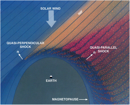
FIGURE 3.1 Schematic showing Earth’s quasi-perpendicular and quasi-parallel bow shock. Shock normal is indicated by the arrow labeled “n.” Adapted, with permission, from B.T. Tsurutani and P. Rodriguez, Upstream waves and particles: An overview of ISEE results, Journal of Geophysical Research 86(A6), 4319-4324, 1981. Copyright 1981, American Geophysical Union.
the shock to satisfy the Rankine-Hugoniot conditions (the mathematical conditions that describe the changes in plasma and magnetic field parameters across discontinuities), and thus help establish the structure of the shocks. Also, the energized particles can become major participants in the balance of energy and momentum across the shocks. Given the potentially large gyroradii of such particles, the structure of the shocks can be further modified and thickened.
Studies of Earth’s bow shock have resulted in an excellent base of understanding for shock dissipation and shock acceleration in collisionless plasmas. However, the range of parameters represented by planetary bow shocks is limited. A critical uncertainty concerns the influence of particle acceleration and other dissipation processes on the structure of different kind of shocks, including (1) shocks associated with comets, where pickup and other neutral gas interactions play a role; (2) the solar wind termination and heliospheric boundary shocks, where strong particle acceleration may play a role; and (3) very strong astrophysical shocks associated with supernova remnants.
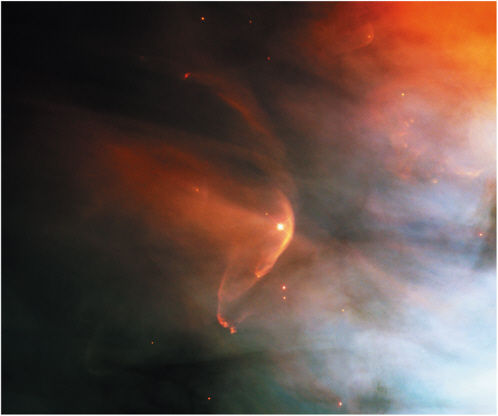
FIGURE 3.2 Bow shock upstream of the young star LL Ori, which is located some 1500 light-years from Earth in the star-forming region of the Orion Nebula. Courtesy of C.R. O’Dell (Vanderbilt University) and the Hubble Heritage Team (NASA/ STScI/AURA).
Outstanding Questions About Collisionless Shocks
-
How do strong particle acceleration and associated energetic particles modify shock structure?
-
How do pickup and other neutral gas interactions modify shock structure and particle acceleration at comets and heliospheric boundary shocks?
-
How do researchers extrapolate knowledge of shock structure derived from studies of solar system shocks to the strong shocks that prevail in astrophysical systems?
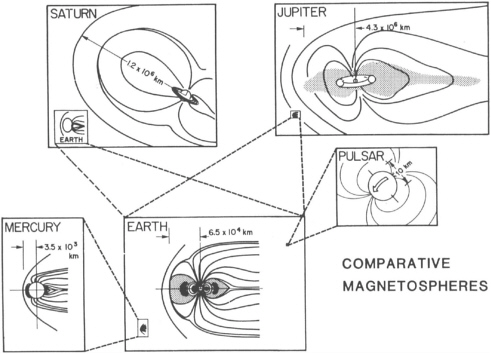
FIGURE 3.3 Magnetospheres epitomize the cellular organization of astrophysical plasmas.
CELLULAR STRUCTURES AND CURRENT SHEETS
Cellular Structures
Magnetized plasmas in space tend to form cells enclosed by current sheets. “We find that space occupied by plasmas tends to be divided in ‘compartments,’ often separated by thin current sheets. On the interstellar and intergalactic scale, space may have a cellular structure consisting of many separate regions, containing plasmas of different magnetization, density, temperature, and perhaps also different kinds of matter.”3 Figure 3.3 shows a hierarchy of magnetic cells in the form of various magnetospheres.
Cells form when magnetized plasmas from spatially separated origins, pursuing their natural, expansionist tendencies, collide, or compete for the same space. The surface along which the competing plasmas meet, which ideally is a current sheet, can be thought of as the cell wall. If the competition produces a stationary (or quasi-stationary) standoff with one side enveloping the other, the notion of a cell is especially apt.
Planetary Magnetospheres
In the solar system, planetary magnetospheres epitomize cellular structures. When the solar wind encounters a strongly magnetized planet that is surrounded by a plasma, the boundary that separates the solar wind and the localized plasma is called a magnetopause. Magnetopauses exist at Earth, Jupiter, Mercury, Saturn, Uranus, and Neptune (Figure 3.4) and should exist at any magnetized body immersed in a stellar wind. Inside the magnetopause is a vast volume that is dominated by the plasma and magnetic field associated with the planet, while outside the magnetopause the solar wind’s plasma and magnetic field dominate. Similarly, a magnetopause can separate planetary magnetospheric plasmas from those confined to the vicinity of a planetary satellite, as in the case of Ganymede in Figure 3.4.
For Earth’s magnetosphere, the problem of the gross structure of the magnetopause was first solved in the early 1960s in a restricted form known as the Chapman-Ferraro solution. In this restricted form, the size and shape of the magnetopause are determined by the ram pressure of the solar wind and the strength of the planetary magnetic dipole and its orientation relative to the solar wind. Chapman-Ferraro scaling for size is well satisfied for Mercury, Saturn, Uranus, and Neptune. Jupiter deviates markedly from Chapman-Ferraro scaling. At this massive planet, internal particle pressure plays a major role and therefore violates the Chapman-Ferraro assumption that the magnetosphere is a vacuum. Chapman-Ferraro scaling does not apply to Venus and Mars because they lack significant internal magnetic fields. Although Venus, Mars, and comets do not satisfy this Chapman-Ferraro scaling, they do generate a cellular structure with a leading shock because they are immersed in the supersonic solar wind.
The Heliosphere
The entire solar system resides within a grand plasma cell called the heliosphere, which constitutes a bubble of plasma within the interstellar medium (Figure 3.5). The detailed interaction between the local interstellar medium (LISM) and the solar wind is not well understood, in part because many of the pertinent physical parameters of the LISM are poorly constrained. As the solar wind expands into the LISM, the complex boundaries of the bubble shield us from the interstellar plasma and magnetic fields and most of the cosmic rays and dust that compose the LISM. Indirect evidence and models suggest the following heliospheric boundaries. The supersonic solar wind eventually decelerates to subsonic speeds via a shock—the solar wind termination shock. This structure, to be encountered by the Voyager probes, our most distant spacecraft, is predicted to lie some 100 AU from the Sun. Beyond the termination shock, a boundary layer, the heliopause, exists were the shock-heated solar wind is cooled and diverted as it encounters the LISM flow. Because of uncertainty with respect to the role of the intergalactic magnetic field and very energetic particles in the LISM, it is currently not known whether the LISM flow is supersonic or subsonic. If supersonic, then, like the solar wind deceleration at a planetary shock, the LISM also decelerates via a shock, and the system is referred to as a two-shock model (i.e., bow shock plus termination shock). By contrast, a subsonic LISM does not require a bow shock, and the system is described as a one-shock model.4
Very detailed and sophisticated models that include the self-consistent coupling of plasma and neutral atoms (both interstellar and heliospheric) have been developed over the past several years, and these models are beginning to be used to investigate the stellar-wind-dominated regions (asterospheres) surrounding stars other than the Sun. In this respect, the very detailed plasma physics of the solar wind/LISM interaction has opened up a new field of astrophysics, in which recent observations of Lyman-α absorption profiles toward nearby stars have been interpreted in terms of the interaction of stellar winds with a partially ionized interstellar medium.5
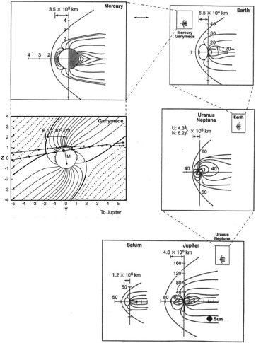
FIGURE 3.4 Schematic diagram showing the magnetospheres in the solar system that result from the interaction of the solar wind with the intrinsic magnetic field of the planets, and, for the case of Ganymede, from the interaction between Jupiter’s magnetospheric plasmas and those confined to the vicinity of Ganymede. In the Ganymede schematic, the thick line separating dashed (magnetic field lines unconnected to Ganymede) and solid (Ganymede-connected) field lines constitutes the magnetopause analogue. The radii (in kilometers) of the planets, moon, and Sun represented are RM = 2436, RG = 2631, RE = 6378, RN = 24874, RU = 26150, RS = 60272, RJ = 71434, Rsun = 695,990. Note (bottom panel) the size of the Sun relative to the jovian magnetosphere, which is the largest object in the solar system. Courtesy of D.J. Williams (Applied Physics Laboratory). The panel showing Ganymede’s magnetosphere is adapted, with permission, from Figure 3 of M.G. Kivelson et al., The magnetic field and magnetosphere of Ganymede, Geophysical Research Letters 24(17), 2155-2158, 1997. Copyright 1997, American Geophysical Union.
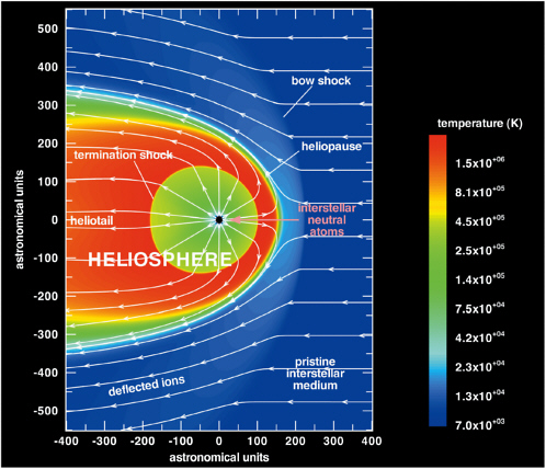
FIGURE 3.5 Simulation of the interaction of the heliosphere with the local interstellar medium (LISM). Whether a bow shock forms upstream of the nose of the heliosphere depends on whether the velocity of the LISM relative to the heliosphere is supersonic or subsonic, which is not known. The magnetized interstellar plasma is excluded from the heliospheric cavity and flows around it. However, interstellar neutral atoms can pass freely through the heliopause. Once in the heliosphere, some of them are ionized by charge exchange with solar wind protons, picked up by the solar wind, and carried back toward the termination shock. At the shock some of the pickup ions are accelerated to extremely high energies and return to the inner heliosphere as anomalous cosmic rays. Image courtesy of V. Florinski (University of California, Riverside). Reprinted, with permission, from V. Florinski et al., Galactic cosmic ray transport in the global heliosphere, Journal of Geophysical Research 108(A6), 1228, doi:10.1029/2002JA009695. Copyright 2003, American Geophysical Union.
Current Sheets
The controlling agents in the formation and maintenance of the cellular structure of solar system plasmas are current sheets. By definition, a current sheet carries a significant electrical current within a two-dimensional (sheet-like) structure. The term “current sheet” implies a structural lifetime much longer than characteristic plasma time scales (e.g., gyroperiod, plasma period), thus distinguishing it from plasma wave structures. And it implies a structure that moves only slowly with respect to the plasma, thus distinguishing it from shocks. The current in current sheets may be oriented either perpendicular to the magnetic field or parallel to it, and the distinction between perpendicular and parallel current sheets is not always a clean one.
Three distinct processes produce sheets of perpendicular current, in which the current density J is largely perpendicular to the magnetic field B. The first process involves the collision between two plasmas. The intervening current layer typically collapses to a sheet having a thickness close to the gyroradius of the dominant ion. Familiar examples include the dayside magnetopause of a planetary magnetosphere, the dayside ionopause of an unmagnetized planet (in analogy to the magnetopause at a magnetized planet), the boundary between solar-wind streams of different properties, and (presumably) the as-yet unexplored heliopause. A second process by which current sheets are produced is the stretching and dragging of magnetic flux tubes downstream by a flowing plasma. These flux tubes are anchored to a stationary obstacle in a background flowing plasma, forming two adjacent lobes of oppositely directed flux. The current sheet resides between the two adjacent lobes. This process occurs in planetary magnetotails, in cometary ion tails, and in the analogous induced magnetotails that appear downstream of an unmagnetized planet or satellite with a conducting atmosphere that is immersed in a flowing magnetized plasma (e.g., Venus, Mars, Titan). A third current-sheet production mechanism involves the inflation of a quasi-dipolar field by internally generated plasma stresses. An example of the agent of inflation can be the centrifugal acceleration of partially corotating plasma in a rapidly rotating magnetosphere like that of Jupiter and perhaps Saturn. A prominent example of the third mechanism is the heliospheric current sheet formed by the outflowing solar wind (Figure 3.6).
With the three basic kinds of dynamically created current sheets, the currents flow with a large component that is perpendicular to the magnetic field vectors on each side of the sheets. Sheets of parallel current (J∥B to a good approximation) are also ubiquitous but arise from different causes and have different effects. An example is the current sheets associated with the northern and southern lights, the auroras.
Magnetopause current sheets arise naturally, for example, in all magnetohydrodynamic (MHD) models of planetary magnetospheres. Other current sheet structures are not so well understood. Jupiter’s magneto-disk is one such structure. In general, it is not known which forcing terms (e.g., the centrifugal force) dominate in the fully developed magnetodisk and therefore how the magnetodisk current is generated. Pressure gradients, pressure anisotropies, field-aligned plasma acceleration, and beaming effects can all contribute, and the evolution of the current sheet can redistribute the importance of the various terms.
Across the domain of all current sheets, the greatest immediate challenge lies in the coupling that occurs between small and large scales, both in the temporal and spatial domains. Current sheets are the sites where the different interacting scales of a magnetized cosmic structure come together and influence each other.
Outstanding Questions About Current Sheets
-
What factors determine the stability and instability of current sheets?
-
How does Jupiter’s unique magnetodisk form and how is it supported?
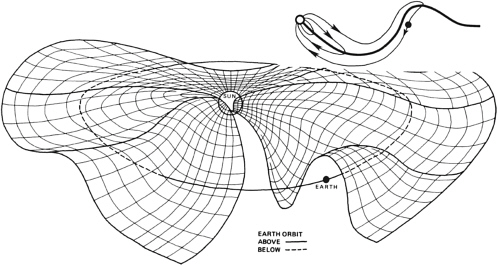
FIGURE 3.6 Schematic diagram of the three-dimensional structure of the current sheet that flows in an azimuthal direction around the Sun. The inset at the top of the figure shows the opposite polarities of the magnetic fields on the two sides of the current sheet. Courtesy of S.-I. Akasofu, Geophysical Institute, University of Alaska.
CURRENT SHEET STRUCTURING: BOUNDARY LAYERS AND FLUX ROPES
The separation of the plasma cells by current sheets and, where applicable, the accompanying shocks, is not perfect. Current sheets are often inherently dynamic, and they tend to form smaller-scale structures that are often dissipative. Dissipative processes allow energy and mass to be transported across the boundary. Processes that work toward the dissipation and destruction of current sheets are reconnection, tearing instabilities, impulsive penetration across boundaries by fast-flowing, high-density or high-pressure plasma blobs, the Kelvin-Helmholz instability, non-adiabatic particle acceleration, and the coupling to adjacent regions by field-aligned currents and the associated shear-stresses within the magnetic field. An important consequence of this structuring is the formation of boundary layers at current sheets. Examples of boundary layers formed by structuring are Earth’s low-latitude boundary layer and high-latitude mantle. Such boundary layers often have sheared plasma flows, magnetic field-aligned particle streaming, and strong particle pressure gradients extending substantial distances from the current sheet proper.
Current sheet structuring can also cause some current sheets to periodically or sporadically disappear altogether. An example is the earthward diversion of the current sheet within Earth’s magnetotail during the dynamical events called substorms. The current sheet dissipative processes listed above can generate specific classes of spatial structures. Chapter 2 discusses boundary layers generated at Earth’s magneto-pause and within Earth’s magnetotail by magnetic reconnection. This section focuses on a specific class of
current sheet structuring—flux ropes—because of its general applicability and importance for plasmas throughout the solar system, and presumably beyond.
A magnetic flux rope is a magnetic field configuration with the following characteristics: (1) locally tubular geometry, (2) helical magnetic field lines with zero twist on the axis and a pitch angle increasing from zero with increasing distance from the axis, and (3) maximum field strength on the axis. This qualitative geometrical definition of a magnetic flux rope does not specify the plasma characteristics, the global magnetic field topology, or the generation mechanism. Magnetic flux ropes can be found in the laboratory, in a variety of places in the solar system, and in other astrophysical settings. The geometry of the magnetic field in a flux rope implies the existence of a component of current along the magnetic field lines. These structures can be generated by magnetic reconnection and other plasma processes.
One of the earliest applications of flux ropes to solar physics was the Gold-Hoyle theory of solar flares, which proposed a model of flux ropes with constant twist.6 Since then, the concept of flux ropes has grown enormously in importance for interpreting solar phenomena (Figure 3.7). Solar active regions themselves are now considered to be manifestations of large flux ropes. It is widely held that each bipolar active region is a single flux rope that has risen buoyantly through the convection zone from a dynamo layer.7
Flux ropes are observed in the solar wind as the magnetic field configuration within magnetic clouds. Magnetic clouds are defined as transient ejecta with (1) greater than average magnetic field strengths, (2) a smooth rotation in magnetic field direction, and (3) low proton temperatures and β (the ratio of plasma to magnetic pressure). They are a particularly well-organized type of coronal mass ejection. Globally, the magnetic clouds observed near 1 AU have the form of loops or ropes typically with both ends connected to the Sun (Figure 3.8).8 Small magnetic flux ropes, with diameters 10 to 40 times smaller than those of magnetic clouds (i.e., 1-4 × 10⁶ km), have recently been observed in the solar wind. These flux ropes differ from magnetic clouds in several respects, and they probably have an origin different from that of magnetic clouds.
More than 20 years ago flux ropes were discovered in the ionosphere of Venus.9 These were observed as a series of large magnetic field strength enhancements, many with a ratio of maximum to minimum field strength of the order of 50. They are more numerous at lower altitudes, suggesting that either they form there and rise buoyantly or they form near the ionopause and are dragged toward Venus by the interplanetary magnetic field to which they are connected.
In the mid-1980s evidence was found for the existence of flux ropes in the distant geomagnetic tail, »100 RE downstream from Earth.10 The flux ropes were initially identified on the basis of a south-then-north tilt of the magnetic field, a strong core field, and a significant east-west component of the field in “plasmoids” moving at several hundred kilometers per second down the tail. An association with substorms was noted. Other flux rope structures have been observed more recently within the magnetotail. Several mechanisms for the formation of flux ropes in the magnetotail have been proposed,11 but the favored hypothesis is magnetic reconnection at near-Earth and distant neutral lines.
Magnetic flux ropes have been discovered in many different locations in the solar system, and they undoubtedly occur in many other astrophysical systems. They may have a common geometrical form, but depending on boundary conditions and temporal evolution, they will differ to varying degrees from this form. Flux ropes and the boundary layers from which they can arise share a number of fundamental physical problems and questions.
Outstanding Questions About Boundary Layers and Flux Ropes
-
How are mass and energy transported across collisionless boundary layers?
-
What factors cause current sheets and boundary layers to form flux rope structures?
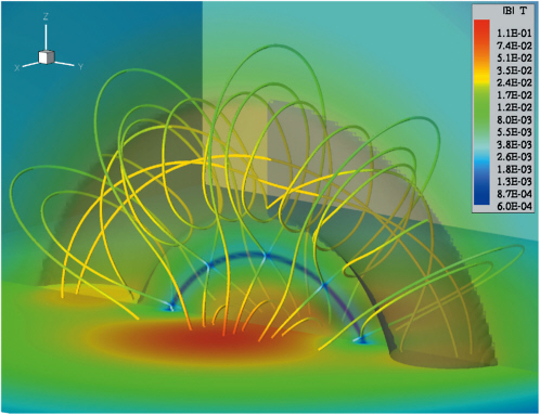
FIGURE 3.7 Computer simulation of a flux rope in the solar corona. The false color indicates the magnetic field strength in teslas. Image courtesy of I. Roussev (University of Michigan). Reprinted, with permission, from I.I. Roussev et al., A three-dimensional flux rope model for coronal mass ejections based on a loss of equilibrium, Astrophysical Journal 588, L45-L48, 2003. Copyright 2003, American Astronomical Society.
-
Under what conditions are flux ropes stable and unstable?
-
What is the relationship of flux ropes to reconnection?
-
How do flux ropes evolve and what determines their sizes?
-
How are flux ropes destroyed?
CROSS-SCALE COUPLING
Flux ropes are just one important class of structures that demonstrate the fundamental propensity of plasmas to couple strongly across multiple scales. This property of magnetized plasmas has important
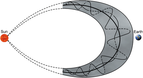
FIGURE 3.8 Magnetic flux rope in the form of a “magnetic cloud” from the Sun. Modified, with permission, from L. Burlaga, Global configuration of a magnetic cloud, pp. 373-377 in Physics of Magnetic Flux Ropes, Geophysical Monograph 58, C.T. Russell, E.R. Priest, and L.C. Lee, eds., American Geophysical Union, Washington D.C., 1990. Copyright 1990, American Geophysical Union.
implications for structures in plasmas and plasma dynamics. Cross-scale coupling in a plasma can be coherent or turbulent. In a coherent interaction, a specific wave mode generated by free energy in a plasma affects macroscopic plasma parameters by a microscopic, direct, resonant interaction (e.g., a wave-particle resonant interaction). Coherent coupling between microscopic and macroscopic scales presents a profound challenge to space plasma theory and modeling. It is often difficult to understand the microscopic plasma processes because they result from complicated boundary conditions imposed by the macroscopic system and because they are normally observed in a state of nonlinear saturation, which is difficult to treat theoretically. Furthermore, the microscopic process has a controlling influence on the large-scale situation, so that the system must be treated self-consistently. Examples of coherent coupling include magnetic reconnection, the generation of monochromatic Kelvin-Helmholtz waves on the magnetopause, and the generation of quiet auroral arcs from large-scale plasma flows.
At the opposite extreme is turbulent coupling, where many dynamical modes of the system are simultaneously stimulated and interact strongly. The most active states of the aurora, where no dominant spatial scale can be found, undoubtedly involve turbulent coupling. Although turbulence is in a saturated state, turbulent processes also evolve and must be treated over a large range of scales. Hydromagnetic turbulence, a special case of turbulent coupling in space plasmas, is discussed in some detail in this section as an example of the challenges to understanding this fundamental plasma process.
Hydromagnetic Turbulence
Probably the most well-studied example of cross-scale coupling in a plasma is hydromagnetic turbulence. Turbulence is a broadband, nonlinear dynamical interaction of fluctuating quantities (e.g., velocity) at multiple scales in a fluid, magnetofluid, or plasma. Larger scales tend to feed energy to smaller scales and this “cascade” process continues down to a dissipation scale, where heating occurs. As generally understood, the reason that energy transfers to small scales through the cascade process is simply that waveforms or structures steepen and stretch owing to one flow or current system shearing and compressing another.
Examples of turbulent dissipative processes are found in the small-scale magnetic interactions in the chromosphere and transition regions of the solar atmosphere and their possible coupling to the corona and solar wind. Furthermore, the solar wind itself has been observed to evolve toward a fully MHD turbulent state as it propagates toward the magnetosphere. In the magnetosphere, thin boundary layers such as the magnetopause are unstable to turbulent plasma processes. Nonlinear growth and saturation of these processes may lead to enhanced particle transport and heating. Turbulence apparently plays an important role in current disruptions and bursty bulk flows in Earth’s magnetotail and in their correlation with large magnetic field fluctuations. Finally, turbulence plays an important role in dynamo processes (see Chapter 2).
Turbulence has been studied most completely in the solar wind.12 The characteristic spectra of turbulence are observed over a few decades of scales in solar wind magnetic fields, velocities, densities, and temperatures, and these spectra evolve with distance from the Sun. Fundamental questions concerning turbulence remain even as it relates to the well-studied solar wind. These questions relate to turbulence spectra and their evolution, cascade rates, symmetry, and “Alfvénicity” correlations.
The most frequently cited characteristic of turbulence is a k−5/3 spectrum of any quantity (e.g., velocity) as a function of the magnitude of the wave vector, k, in the medium. Kolmogoroff derived this spectrum in 1941 for the velocity field in an isotropic, high-Reynolds-number (low-viscosity) fluid.13 He used dimensional arguments for the “inertial range” of wave numbers (k’s) in which viscosity is unimportant compared to nonlinear terms. Viscosity set the dissipation scale, and the large, “energy-containing” scales decayed at a slow but predictable rate. For unknown reasons, the −5/3 spectrum is observed in the solar wind despite the fact that it is inhomogeneous, is anisotropic, and contains a magnetic field that could slow the interactions and flatten the spectrum.
The turbulent spectral level determines the steady-state cascade rate of energy from one scale to the next in the Kolmogoroff formalism. Energy conservation implies that the cascade rate is equal to the dissipation rate. These turbulence constraints can be used to compare predicted and observed heating of the solar wind. In general, predictions and observations agree reasonably well with respect to the evolving solar wind in the inner heliosphere. However, attempts to use phenomenological cascade rates to account for heating of the corona and acceleration of the solar wind suffer from uncertainties in the fluctuation levels. In particular, it is not clear that fluctuations can be generated at high enough levels to account for the observed coronal heating.
The magnetic field plays an important role in creating symmetry. Fluctuations with wave vectors along the mean magnetic field are much more effective in scattering particles than are those with wave vectors nearly transverse to the field. The interplanetary fluctuations may contain significant levels of the quasi-two-dimensional fluctuations associated with both fields and wave vectors perpendicular to the mean field. Cascades are more effective perpendicular to the mean field, since parallel fluctuations must bend the field lines. Thus, it is unlikely that space plasmas have isotropic fluctuations, and spectra may vary in different directions (recent studies suggest such anisotropy). The results of further study of symmetry will be important for understanding cosmic-ray modulation and solar energetic particle propagation.
Coherent cross-scale coupling occurs in a variety of regions within the heliosphere. Important questions concerning coherent coupling processes such as reconnection at Earth’s magnetopause are posed in Chapter 2. Significant questions remain, too, on the origin, evolution, and role of turbulence in space plasmas. Often the most promising approach to the study of turbulence is simulation coupled with the observation of real plasmas. Various models of turbulence also show promise, although they must be continually checked against simulation and observation for success. Answering these questions will enhance our understanding of turbulence in general, thus increasing our ability to apply our ideas to astrophysical situations where direct measurements are not possible.
Outstanding Questions About Cross-Scale Coupling and Turbulence
-
What is the detailed structure of heliospheric turbulence, and what are the consequences of this structure for the propagation of energetic particles?
-
To what extent is observed turbulence actively cascading as opposed to being a “fossil” record of prior nonlinear processes?
-
Does turbulent heating play a significant role in any of the main areas that have been suggested, namely the corona, the heliosphere, and Earth’s magnetosphere?
-
What is the mechanism for the dissipation of turbulence?
UNIVERSALITY OF STRUCTURES AND TRANSIENTS
Structures and transients are ubiquitous in the observable universe and play key roles in the redistribution of energy and momentum. The challenge is to determine the processes responsible for generating them. Further, it is important to understand how these processes are modified by vastly different scales and external boundary conditions in astrophysical settings. Astrophysical shocks are an example of this challenge. Earth’s bow shock and a shock at a supernova remnant are distinctly different structures. However, understanding how interplanetary shocks differ from Earth’s bow shock and how the heliospheric termination shock differs from interplanetary shocks leads to an understanding of how shock structure is modified when the pressure is dominated by a very energetic particle population. This understanding can then be extended to extreme cases such as shocks at supernova remnants.
There are other structures where analogies may reveal themselves through joint study. Do the fine tendrils observed within the Crab Nebula carry electric current, and are they analogous to the current filaments responsible for generating the aurora? Are the bipolar jets that are thought to help carry away angular momentum from collapsing protostars analogous to the auroral discharges at Jupiter, similarly responsible for shedding angular momentum (albeit small amounts) from that spinning body?
There are also important analogies between turbulence in the solar wind and in the diffuse interstellar medium. Resolving important questions concerning turbulence in the solar wind will provide important insight into the properties of the interstellar medium. Extending our understanding of turbulence in these regimes to other environments, such as star-forming regions in dense molecular clouds, is also important. In these regions, it appears that the turbulent energy decay rates are found to scale much the same way as in the heliosphere. This turbulence may play a role in stochastic acceleration of charged particles, becoming a possible mechanism of reacceleration of cosmic rays in the Galaxy.
The universal tendency of plasmas to couple across scales is exemplified by magnetic “islands” found in structures as different as astrophysical jets and the boundary layers of Earth’s magnetosphere. Some aspects of such islands, as seen in the optical image of Quasar 3C 273 (Figure 3.9), have been attributed in similar jets to driven Kelvin-Helmholtz instabilities, while the x-ray emissions have been associated
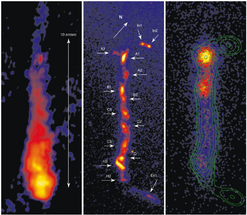
FIGURE 3.9 Images of an astrophysical jet from Quasar 3C 273 in ground-based radio (1.647 GHz), Hubble optical (617.0 nm), and Chandra x-ray (with optical overlay) bands. Features are labeled in the Hubble image as noted by J.N. Bahcall, S. Kirhakos, D.P. Schneider, R.J. Davis, T.W.B. Muxlow, S.T. Garrington, R.G. Conway, and S.C. Unwin, HST and MERLIN observations of the jet in 3C273, Astrophysical Journal 452, L91-L93, 1995. Courtesy of H. Marshall (Massachusetts Institute of Technology). Reprinted, with permission, from H.L. Marshall et al., Structure of the x-ray emission from the jet of 3C 273, Astrophysical Journal 549(2), L167-L171, 2001. Copyright 2001, American Astronomical Society.
with shocks that form as the supersonic jet is slowed by interactions with the ambient medium. The x-ray emissions from the jet islands could also be caused by particles accelerated in magnetic reconnection events. Similar island formation occurs in plasma boundary layers in the terrestrial magnetosphere (Figure 3.10). These islands can be caused by Kelvin-Helmholtz MHD instabilities or by ion-tearing instabili-
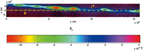
FIGURE 3.10 Magnetic islands along Earth’s magnetopause deduced from in situ magnetic field data. These islands have been attributed to the ion-tearing mode. Reprinted, with permission, from L.-N. Hau and B.U.Ö. Sonnerup, Two-dimensional coherent structures in the magnetopause: Recovery of static equilibria from single-spacecraft data, Journal of Geophysical Research 104(A4), 6899-6918, 1999. Copyright 1999, American Geophysical Union.
ties and the associated magnetic reconnection. As these examples show, magnetic island structures resulting from high-speed differential plasma flows are present in both astrophysical and heliospheric environments, although at vastly different parameter scales. Even so, common phenomena such as MHD instabilities, shocks, and magnetic reconnection have been invoked to explain the structures in both environments.
Despite the vast differences in parameter regimes and boundary conditions that distinguish solar system and astrophysical plasma structures, the underlying plasma physical processes that give rise to and power these structures are the same. Ultimately, a fuller understanding of these processes in a general sense should be obtained with contributions from both space physics and plasma astrophysics.


