
6
Assessing Potential Effects on the Electricity-Generating Sector1
INTRODUCTION
As explained in Chapter 4, of all the affected sectors, electric-power generation is the best candidate for the use of a sectorwide simulation model to assess the potential efficiency, technology, and emission implications of New Source Review (NSR) rule changes. In this chapter, we use the electricity-sector model referred to as the Integrated Planning Model (IPM) to bound some of the possible effects of the NSR equipment replacement provision (ERP), the principal change that was to affect the power-generation industry. We define a set of runs of IPM that represent different scenarios concerning the effects of the rule, other interacting air regulations, and background economic and technological conditions. We then compare and interpret the results.
The analyses presented in this chapter were undertaken before the recent appellate court decision struck down the ERP (see Chapter 2 for a discussion of that decision). It is important to keep in mind that the model simulations of the ERP can also be interpreted as simulations of the U.S. Environmental Protection Agency’s (EPA’s) hourly emission test (see Chapter 2), because no electricity-generating facilities in the ERP analyses are allowed, according to the analytical procedure used by the committee, to make changes that result in an increase in the maximum hourly emission rate, and so all are in com-
pliance with the hourly emission test proposal. Consequently, the analyses of this chapter are relevant to any comparison of NSR prior to proposal of the ERP with the EPA hourly emission test proposal.
The arrangements for the IPM model runs were coordinated through the EPA because of the nature of EPA’s contractual relationship with ICF Consulting, the owner of IPM. The committee provided scenarios to EPA, and EPA in turn provided the scenarios to ICF and oversaw the implementation of the model. The results of the model runs were then checked for errors by EPA employees and provided to the committee. The committee independently analyzed the results by creating graphs and tables and doing cross-scenario comparisons.
The modeling effort is intended to build on the earlier modeling work done by EPA as a part of its regulatory impact analysis (RIA) of the adoption of the ERP (EPA, 2003c). Our analysis looks at a wider range of potential effects upon generation investment decision making under the agency’s prerevision NSR multifactor approach than were examined as part of EPA’s RIA. Furthermore, unlike the EPA analysis, which was prepared before the Clean Air Interstate Rule (CAIR) and the Clean Air Mercury Rule (CAMR) (see Chapter 2) were to be put into place, our analysis takes into account the effects of those rules on industry’s response to the NSR changes.2 The design of these runs and their rationale are reviewed in detail in the next section. After reviewing the results, we discuss the limitations of the model and any conclusions based on them. A set of conclusions closes this chapter.
Table 6-1 summarizes the emission-control status of U.S. coal-fired units in 2004. The focus of our analysis is on the 188.5 gigawatts (GW) of large electricity-generating units (at least 100 MW) that as of 2004 lacked flue-gas desulfurization (FGD) controls for sulfur dioxide (SO2) and on the 190.4 GW of large units that as of the same year lacked selective catalytic reduction (SCR) or selective noncatalytic reduction (SNCR) controls for nitrogen oxides (NOx). That focus is based on our assumption that this capacity constitutes the bulk of power-sector emissions that would potentially be affected by the ERP approach. Those uncontrolled units account for 62% and 63%, respectively, of all coal-fired generation capacity. Our analysis excludes 17 GW of smaller units (less than 100 MW), or about 6% of all coal-fired capacity, on the assumption that they would not be suitable candidates for retrofit of FGD or SCR; we assume that those units avoid undergoing NSR.
TABLE 6-1 Installed Emission Controls, U.S. Coal-Fired Generation Plants, 2004
|
NOx Controla |
SO2 Control |
Capacity (MW) |
% Capacity in Group |
Number of Boilers |
% of Boilers in Group |
|
Large (≥ 100 MW) generating units |
|||||
|
None |
None |
126,640 |
45% |
432 |
56% |
|
None |
Dry scrubber |
9,574 |
3% |
28 |
4% |
|
None |
Wet scrubber |
54,259 |
19% |
123 |
16% |
|
SCR |
None |
54,146 |
19% |
105 |
14% |
|
SCR |
Dry scrubber |
2,002 |
1% |
6 |
1% |
|
SCR |
Wet scrubber |
27,066 |
10% |
45 |
6% |
|
SNCR |
None |
7,232 |
3% |
29 |
4% |
|
SNCR |
Dry scrubber |
248 |
0% |
1 |
0% |
|
SNCR |
Wet scrubber |
1,461 |
1% |
6 |
1% |
|
Total for large units |
282,628 |
100% |
775 |
100% |
|
|
Small (< 100 MW) generating units |
|||||
|
None |
None |
16,333 |
80% |
386 |
84% |
|
None |
Dry scrubber |
1,773 |
9% |
33 |
7% |
|
None |
Wet scrubber |
710 |
3% |
17 |
4% |
|
SCR |
Wet scrubber |
254 |
1% |
3 |
1% |
|
SNCR |
None |
737 |
4% |
12 |
3% |
|
SNCR |
Dry scrubber |
310 |
2% |
6 |
1% |
|
SNCR |
Wet scrubber |
263 |
1% |
5 |
1% |
|
Total for small units |
20,380 |
100% |
462 |
100% |
|
|
aSCR means selective catalytic reduction. SNCR means selective noncatalytic reduction. |
|||||
DEFINITION OF SCENARIOS
The IPM scenarios are specified on three dimensions. One dimension consists of different versions of EPA’s policy regarding the breadth of the routine maintenance, repair, and replacement (RMRR) exemption from NSR with different assumptions about its strictness or direct effects on electricity-generating facility decisions. A second dimension represents assumptions about what other air-pollution regulations will be in place. The third dimension consists of alternative scenarios about economic and technological conditions, such as growth in the demand for electricity, fuel prices, and investment costs for different electricity-production and pollution-control technologies.
Dimension 1: Strictness of Prerevision Routine Maintenance, Repair, and Replacement Policy
IPM, like all national-scale models of the electricity-generating facility sector, does not explicitly represent the full range of life-extension and
maintenance alternatives available to power-plant owners, nor does it have data available on the site-specific costs of such alternatives. As a result, IPM cannot explicitly model how the EPA RMRR policy changes the alternatives that individual plants can consider or how the provision affects their costs, and it is not possible for such a model to project with confidence what individual power plants will do under alternative versions of RMRR policy. However, we can hypothesize different levels of aggregate effects of RMRR policy on generating-plant costs, efficiency, and adoption of pollution controls and then use IPM to examine how the industry might have responded in terms of generator retirement, mix of new generation, and emissions. In particular, the strictness of the prerevision NSR RMRR might be characterized in terms of the following:
-
How much coal-fired generating capacity is compelled to upgrade to best available control technology (BACT), repower (to combined-cycle capacity, fired either by natural gas or by integrated coal gasification), or retire as a result of NSR review or the threat of such review.
-
How much capacity will instead face mild performance deterioration as a result of deferring maintenance rather than undergoing NSR.
-
How many allowances would be surrendered as a result of NSR settlements.
As a first step, we simplify the NSR policies into two basic alternatives: the prerevision NSR multifactor approach and the ERP adopted in 2003. We then define variants of industry response to the prerevision NSR approach to represent different assumptions about the possible effects that the previous approach could have had on post-2004 generator decisions about maintenance, retrofits, repowering, and retirement. These cases span a wide range of possibilities, from all nonscrubbed coal-fired generators deciding in the future to avoid NSR by deferring all maintenance to essentially all such generators retrofitting FGD-SCR systems, repowering, or retiring (R/R/R) by 2020.
Table 6-2 summarizes the various cases. For the prerevision NSR rules, two general variants are defined: (1) “avoid,” in which generators by and large are able to avoid triggering NSR but at the cost of worsening performance (that is consistent with the assumptions of the RIA of EPA [2003c]), and (2) “R/R/R,” in which the outcome would be enforcement policy that leads to substantial amounts of capacity to choose to retrofit FGD-SCR, repower, or retire. The committee has reached no conclusion as to which general variant involves more realistic assumptions. The R/R/R variant assumes that either lawsuits or the possibility of lawsuits will eliminate avoidance of NSR as an alternative for a substantial amount of generation, so that owners must choose between retiring and undergoing NSR; the latter
TABLE 6-2 Summary of NSR Cases Simulated and Assumptions
|
NSR Case |
Which plants must choose between FGD-SCR, retirement, and repowering as the result of NSR? |
Which plants face performance deterioration if they avoid NSR by doing no maintenance or life extension? |
Allowance surrenders as a result of settlements |
|
Previous RMRR variant 1: “Avoid” |
None |
All coal-fired generation |
None |
|
Previous RMRR variant 2: R/R/R |
Specified fraction of pre-1978 coal-fired plants larger than 100 MW; fraction grows linearly from X% in 2008 to 13X% in 2020, with X = 2, 5, 7.5 (“low,” “middle,” “high” variants, respectively) |
Some or none |
No surrenders beyond those in settlements made before March 2004 |
|
2003 ERP |
None |
None |
Same as above |
will result in retrofitting of BACT-compliant emission controls or repowering to BACT-compliant combined-cycle technology. Those general variants represent the range of possible effects on uncontrolled coal-fired capacity that have been put forth by various parties. As noted, the first variant is that which is assumed by EPA (2003c) in its RIA of the 2003 ERP proposal; the other variant is generally consistent with views that have been stated by some stakeholders, including many in the environmental community.3 The committee has determined that economic, policy, and legal uncertainties are too large to determine which variant is most likely to be correct, so we have adopted a scenario and bounding approach to explore the consequences of alternative assumptions.
The R/R/R variant is simulated by imposing the following constraints on the 188.5 GW of pre-1978 coal-fired units that are at least 100 MW and lacked FGD as of 2004 (Table 6-1):4 a lower bound is placed in each model year starting in 2008 on the number of megawatts of such capacity that is either retrofitted with FGD, repowered with BACT-compliant combined-cycle technology, or retired; and an analogous bound is applied to the 190.4 GW of pre-1978 coal-fired units greater than 100 MW that lack
SCR or SNCR, which must either retrofit SCR, repower, or retire. Those bounds simulate a possible outcome of the prerevision NSR RMRR: that some unscrubbed capacity or capacity without SCR would be cleaned up or retired. Variants of the basic alternative assume different levels of the lower bounds, which represent different rates of retrofitting, retiring, or repowering of existing capacity. The lower bounds are tightened over time by increasing the percentage of such capacity that has to make that choice. The first variant (termed the low R/R/R impact variant) assumes that 2% per year of the 188.5 GW of unscrubbed capacity (190.4 GW of capacity without SCR-SNCR) is retrofitted, repowered, or retired in each year from 2007 and 2020. As a result, 2% has been retrofitted by 2008, 4% by 2009, and so forth, reaching 26% in 2020, and flat thereafter.5 This is the equivalent of about 3,700 MW per year of generation either undergoing NSR (retrofit or repower) or retiring, in the case of the SO2 constraint. The two other variants assume 5% and 7.5% growth per year (equivalent to 9,400 MW and 14,100 MW per year of R/R/R in the SO2 case, respectively). The 5%/year scenario (called the middle variant) means that 65% would have been scrubbed, retired, or repowered by 2020, and the 7.5%/year scenario (termed the high variant) reaches 97.5% by 2020. The latter scenario is unlikely because it results in R/R/R substantially above what could credibly occur, because some fraction of uncontrolled generation is likely instead to avoid NSR by deferring maintenance. Furthermore, given the historical rate of scrubber retrofits and the rate of NSR settlements that have already been made, the 14.1-GW/year rate implied by the high variant is large and seems unlikely to be sustainable. Table 5-2 (EIA 2004a) shows that a cumulative 99.6 GW of scrubbers had been installed by 2003, whereas in 1992 there was 71.5 GW, a difference of 28.1 GW in over 2 decades. However, Table 6-3 indicates that owners of electricity-generating facilities capable of producing a total of less than 17 GW have agreed to retrofit scrubbers as the result of NSR enforcement to date. The rate of R/R/R could increase if a few successful enforcement cases persuade the industry that there is no sense in risking enforcement action, but an assumption that 14 GW/year of retrofits could be sustained in every year through 2020 appears extreme. Nevertheless, we analyze the high scenario, treating it as a bounding case.
The rationale for this approach to modeling the R/R/R variant of the previous RMRR is as follows. We are attempting to characterize broadly the potential role of NSR-driven retrofits (scrubbing and SCR) and repowerings and retirements. We distinguish between NSR-triggered retrofits and allowance-triggered retrofits resulting from CAIR or (in the absence of the CAIR) Title IV, enacted as part of the 1990 Clean Air Act amend-
TABLE 6-3 Year of Installation of Emission-Control Retrofits or Repowering Committed to as a Result of Existing EPA NSR Settlements
|
Year |
SO2 Postcombustion Control or Repowering (MW) |
NOx Postcombustion Control or Repowering (MW) |
|
2003 |
326 |
926 |
|
2004 |
3,255 |
4,695 |
|
2005 |
781 |
861 |
|
2006 |
1,985 |
1,377 |
|
2007 |
1,855 |
1,519 |
|
2008 |
1,020 |
1,013 |
|
2009 |
360 |
1,272 |
|
2010 |
2,754 |
600 |
|
2011 |
581 |
1,258 |
|
2012 |
3,565 |
2,234 |
|
2013 |
0 |
433 |
|
Total |
16,482 |
16,188 |
|
SOURCE: Committee analysis of EPA NSR settlements. |
||
ments, and from the NOx state implementation plan (SIP) call of 1998. An allowance-triggered retrofit is defined as one that is adopted in IPM because it is cost-effective under present and future emission-allowances prices; that is, allowance-triggered retrofit is the lowest-cost method of achieving the emission goals embodied in the caps. In contrast, an NSR-triggered retrofit is the amount of capacity that is R/R/R as a result of NSR enforcement or threat of such enforcement but may not be cost-effective for achieving the caps. Where in time, space, and other dimensions CAIR or other caps are binding, we might expect NSR-triggered retrofits to have little effect on national emissions, although there may be some local effects. They might simply displace allowance-driven retrofits, shifting emission reductions in space and time but having relatively small effects on aggregate emissions. Under those conditions, even large differences in the rate of NSR-triggered retrofits would make little difference in overall emissions. But we can imagine a rate of NSR-triggered retrofits that would be great enough to overtake the CAIR rule (or, in its absence, Title IV and the SIP call), in which case some difference in aggregate national emissions might be attributable to the change in the NSR rules.
Therefore, we can think of triggered retrofits as being approximated by a requirement that a specified percentage of existing uncontrolled capacity be retrofitted, retired, or repowered in each year. For example, if the triggered retrofits happened at 5% per year (assuming that 2008 is the first year when retrofits could feasibly take place), then as indicated above, 15% of currently uncontrolled capacity (as of 2004) would be subject to triggered
retrofits (or repowering or retirement) by 2010, 40% by 2015, and 65% by 2020.
The three R/R/R variants of EPA’s prerevision NSR multifactor approach represent different assumptions about the pace and effectiveness of enforcement. When estimating the costs of implementing the specified fraction of R/R/R, this method should provide an estimated lower bound on cost because the lowest-cost method of meeting the constraint is chosen. This lower-bounding approach allows the model to choose which uncontrolled plants must scrub, retire, or repower on a lowest-cost basis, which of course may not be how EPA chooses plants to be subject to enforcement actions. However, because we cannot predict precisely which generating units will be subjected to such actions in the future or would for other reasons choose to retrofit, retire, or repower and in what order, the use of the lower bound is a simple and transparent way to simulate the possible effect of enforcement of the previous RMRR on power plants.
Because NOx and SO2 emission caps are binding in many years in the simulations, an important assumption concerns the number of allowances that are surrendered as part of enforcement actions. As Table 6-2 indicates, the R/R/R scenarios assume no further allowance surrenders than have already been announced. It is possible that under the prerevision RMRR, additional allowance surrenders could occur. If there would be many more allowances surrendered under prerevision NSR rules, the NOx and SO2 constraints under the SIP call, Title IV, and CAIR would effectively be tighter, and national emissions probably lower. However, it is uncertain whether and how many additional allowance surrenders would have occurred under the prerevision RMRR, and thus, it would be speculative for the committee to estimate how many more would have occurred under different policies. Therefore, we decided to make no specific estimate.
Dimension 2: Other Regulations
The electric-power industry is affected by a number of air-pollution laws at both the federal and state level. There are therefore many potential interactions that could be investigated. The most important are cap-and-trade programs. We defined two alternative other regulations or policies to consider the issue of how NSR would interact with different caps on NOx and SO2 emissions. Those policies are shown as columns in Table 6-4: non-CAIR (present Title IV and NOx SIP call, under the assumption that court or other challenges result in withdrawal of CAIR and CAMR) and CAIR-CAMR, as promulgated by EPA. The CAIR-CAMR simulation includes the best available retrofit technology (BART) provisions associated with the recently promulgated amendments to the regional haze rule (EPA, 2005e). There could be variants on the CAIR-CAMR scenario because there may be
TABLE 6-4 Combinations of NSR ERP Cases and “Other” Air Regulations Simulated
|
NSR Case |
“Other” Case 1: Title IV and NOx SIP Call |
“Other” Case 2: CAIR-CAMR |
|
Previous RMRR variant 1: “Avoid” |
Analysis of effects relative to 2003 ERP based on EPA (2003c) |
Not simulated |
|
Previous RMRR variant 2: R/R/R |
IPM simulations: Three variants run (various lower bounds) |
IPM simulations: three variants run (various lower bounds) |
|
2003 ERP |
EPA (2005e) base case |
EPA (2005e) CAIR-BART-CAMR run |
lawsuits challenging CAIR, which may result in changes in the caps or the timetable. Other developments, such as revised ambient standards for airborne particles, could result in further restrictions. Furthermore, individual states can choose to opt out, although their share of emission reductions (based on Section VII of the preamble to the final CAIR, 70 Fed. Reg. 25255) would still need to be achieved by other means. This could change the spatial distribution of emissions if not the total. However, time and resource limitations meant that we could not consider such variants of CAIR.
The combinations of “other policies” and NSR policies considered in this chapter are shown in Table 6-4. The table also indicates what runs of IPM were used to assess each case. According to EPA statistics, of the 188.5 GW of unscrubbed capacity considered in the R/R/R scenarios, 165.8 GW lies in the CAIR region and an additional 16.5 GW is subject to BART. Of the 190.4 GW of existing non-SCR capacity that is subject to the R/R/R constraint, 144.1 GW is subjected to CAIR and 41.7 GW to BART. Thus, 97% of the capacity subjected to our technology lower bound in the R/R/R prerevision NSR RMRR scenario comes under the CAIR caps or the BART program.6 (Of course, capacity subject to the cap is not required to go through R/R/R.)
Because of budget and time limitations, we used the EPA (2003c) RIA results to represent the “avoid” variant of the previous multifactor test. We do not expect the qualitative results to change significantly if that variant
were rerun. As described in Appendix B of the RIA, IPM simulations assume that in the face of the previous policy, generator owners would opt to avoid undergoing NSR by deferring maintenance. The assumed result would be a steady deterioration of 0.1%/year in efficiency (heat rate) and capacity; in contrast, the RIA assumed that the ERP would increase maintenance, yielding improvements in efficiency, capacity, and, in some scenarios, plant availability. The RIA considered five “increased maintenance” cases with various assumptions. The results showed that the Title IV and SIP emission caps remain binding throughout the entire time horizon of the IPM simulation. Consequently, the deterioration that the RIA assumed in plant capacity and efficiency yielded higher generation costs but essentially the same NOx and SO2 emissions as the “increased maintenance” cases. SO2 emissions varied between the cases by no more than 0.5% in 2010-2020. NOx emissions varied more (by up to 2.5%) because the SIP cap applies only during the ozone season7 and applies to a limited number (22) of states. However, the emission differences between the prerevision NSR rule and the “increased maintenance” cases were 1% or less for most of the cases and years considered because the emission caps are always binding. Therefore, we conclude that the presence of emission caps is what determines the total emissions in the “avoid” variant. Hence, if the prerevision NSR RMRR results in all generators, avoiding NSR, the national NOx and SO2 emission differences between the prerevision RMRR and the proposed ERP would be minor.
EPA (2003c) considered the “avoid” variant only under present SO2 and NOx rules. We expect that a tightening of the emission caps, as promulgated under CAIR, would not change the basic IPM result in EPA (2003c) that an “avoid ERP” strategy of deferred maintenance would leave emissions at the cap and result in higher costs. That is because the logic of market-simulation models, such as IPM, is such that if a constraint is binding in one solution, it will remain binding if it is tightened.8 The magnitude of cost increases would no doubt differ from a non-CAIR scenario, but our main focus here is on the emission effects. Essentially, by making the aggregate emission caps stricter in the East and Midwest and, in the case of NOx, broader in geographic scope, CAIR raises the cost of maintenance deferrals that would increase emissions at individual facilities. Thus, CAIR makes it even less likely that aggregate emissions would be higher under an “avoid ERP” strategy. Given that little was likely to be learned, we chose to forgo the cost of an additional IPM run for a CAIR variant of the “avoid ERP” strategy.
The R/R/R variants are analyzed under both a non-CAIR-CAMR and a CAIR-CAMR regulatory regime with IPM runs undertaken at the request of the committee. The technology, cost, and other IPM assumptions are the same as in the EPA (2005e) analyses of the June 15, 2005, amendments to the Regional Haze Rule. (That rule led to the BART requirements that will lead some western generators, outside the CAIR region, to retrofit with scrubbers and postcombustion NOx controls.) The IPM database did not include the most recent settlements under the NSR rule, but in the committee’s judgment the differences that those settlements would make in the analyses were too small to justify the delay and expense involved in updating the database.9 The limitations and assumptions of the IPM model are discussed later in this chapter.
The last row of Table 6-4 shows that the 2003 ERP is analyzed on the basis of the EPA (2005e) base cases, which assume that under the new rule no further settlements that result in mandatory retrofit of FGD-SCR are made under NSR rules beyond settlements that were in place as of March 2004.10 Those base cases include both non-CAIR-CAMR and CAIR-CAMR scenarios. These are compared with the IPM R/R/R runs (next to last row) to assess possible emissions, cost, and technology effects of the ERP, if it is assumed that the effect of retaining the prerevision NSR approach would
|
9 |
Two recent settlements between EPA and electricity-generating facilities are not in the IPM database, including Ohio Edison (Sammit Units 1-7; Eastlake 4,5; Burger 7,8) and Illinois Power (Baldwin 1,2,3; Havana 6; Hennepin 1,2; Wood River 4,5; Vermillion 1,2). In addition, a state settlement with Mirant is omitted (Potomac River 3,4,5; Morgantown 1,2). A total of 7,805 MW is involved. Of that capacity, 4,936 MW is chosen to be scrubbed anyway as part of the IPM CAMR-CAIR base case run (the run represented by the last cell in the last row of Table 6-3), and 2,869 MW is not (primarily the Baldwin plant). The 2,869 MW is about 1.5% of the total of 188.5 GW of unscrubbed coal capacity in 2004. That small value indicates that omitting those settlements would not greatly distort the solution in that case. IPM also does not have some other recent state NSR settlements. Known examples include the NEG and AES cases in New York. However, these sources may have retrofit anyway in response to state cap-and-trade programs.The other aspect of the recent settlements that is not included in the IPM runs is any systemwide restriction on annual emissions and retirement of allowances. Such retirements would have the effect of lowering the relevant emission caps by the amounts involved. Consequently, national emissions may be overstated in our runs, but because the retirements are small we judge that any such overstatement would not affect our conclusions about the effects of the old NSR RMRR compared with the ERP. For Illinois Power, roughly 30,000 Title IV SO2 allowances must be surrendered each year after 2011. Ohio Edison is required to retire all excess allowances above those that it was initially allocated, but the exact number is not specified in the settlement. |
|
10 |
Whether this assumption is valid depends on future judicial holdings regarding the legality of EPA’s enforcement strategy. An alternative assumption that would not change these solutions is that additional settlements result in retrofits that the generating-capacity owners would have voluntarily undertaken in any event under CAIR-CAMR. |
be to force a substantial amount of nonscrubbed coal capacity to face the R/R/R decision. Those base cases are not compared with the “avoid” scenarios, because the EPA (2003c) RIA IPM runs are based on an earlier set of economic and technological assumptions.
Dimension 3: Alternative Economic, Market, and Technology Scenarios
It was not possible to conduct a thorough set of sensitivity analyses of the cases in Table 6-4 with respect to an array of economic and technology assumptions. Because the IPM analyses indicate that very little uncontrolled coal capacity would be retired by 2020 in any of the scenarios of Table 6-4, we decided to consider whether alternative plausible assumptions might result in more retirements. We focused on the most extreme, bounding R/R/R case (“high,” with a 7.5% increase per year in the amount of uncontrolled coal capacity that must decide to retrofit, repower, or retire) under the CAIR-CAMR scenario.
Natural gas, renewables, and integrated gasification combined cycle (IGCC) were considered because they would be the primary candidates for substituting for retired uncontrolled coal capacity. These sensitivity analyses are performed on the bounding “high” case because it is the scenario in which the prerevision RMRR has the greatest effect on emissions. The “low” and “middle” cases, in which emissions are at the cap in most or all years, would not exhibit as much sensitivity if subjected to the same analyses, because if emissions are at the cap, they are likely to stay at or near the cap.
Two additional IPM runs were specified for the sensitivity analyses using the 7.5% R/R/R case. The first sensitivity analysis had the following changed assumptions relative to the base case assumptions:
-
20% lower investment costs for renewable-energy plants, including wind, solar, landfill gas, biomass, and geothermal.
-
Lower investment costs for IGCC plants: 15% lower in 2010, 20% lower in 2015, and 25% lower in 2020 and 2026. In addition, the capital cost of repowering coal steam to IGCC was lowered by 20%.
The second sensitivity analysis made the same investment-cost assumptions as the first, and assumed lower natural gas prices. That was accomplished by scaling gas-supply curves downward by 15% in 2010, 20% in 2015, and 25% in 2020 and 2026. It should be noted that the base case prices for natural gas in the IPM runs were already low—just over $3.00 per million Btu in $1999, measured at the Henry Hub. In contrast, gas prices that actually prevailed in 2005 were much higher, peaking at about four times that price in October 2005.
We did not consider a scenario with higher gas and investment costs for alternative-energy sources, because such assumptions would yield the same generally low rates of retirement for coal plants as the base case assumptions.
As discussed later in the chapter, we considered the national NOx and SO2 emission reductions occurring under the most extreme (7.5%/year) R/R/R case under CAIR, and calculated the lowest-cost means of achieving those reductions in the same years when they occur. That simulates the use of a policy of caps to achieve the same national emission goals.
RESULTS
Comparison of Emissions
In Table 6-5, we summarize the simulated SO2 and NOx emissions effects of each prerevision NSR RMRR variant (“avoid” and three R/R/R cases) relative to the ERP. These results are discussed in more detail later in this section. Four of the 5 years calculated by the IPM are presented (2007, 2010, 2015, and 2020); 2026 is omitted because the committee judges the last year’s results to be less reliable than those of earlier years.11 As mentioned, the estimated effects in the “avoid” case are based on the EPA (2003c) RIA, which considers only the Title IV and NOx SIP call caps. The R/R/R cases’ effects are calculated by using the IPM runs requested by the committee. The effects are expressed as percentage changes relative to the ERP base case (last row of Table 6-4) for each of the two assumed sets of emission caps. Figures 6-1 through 6-4 present the same results in graphic form, expressed as total tons (Figures 6-1 and 6-2) and tonnage differences between the prerevision NSR RMRR and base case results (Figures 6-3 and 6-4). Those figures show the changes in emissions resulting from the three variants of the R/R/R prerevision NSR RMRR scenario relative to the 2003 ERP base case over the 2007-2020 period under both
TABLE 6-5 Summary of SO2 and NOx Emission Effects of Prerevision NSR RMRR Relative to ERP (Base Case) Under Base Case Economic and Technology Assumptions (Rounded to Nearest Percent)
|
NSR Case |
“Other” Case 1: Title IV/NOx SIP Calla |
“Other” Case 2: CAIR-CAMR, as Promulgateda |
|
Prerevision RMRR policy, “avoid” variant (compared with 2003 ERP from EPA [2003c] RIA) |
ΔSO2 > –1% all scenarios and years (small positive values if ERP assumed to result in increased maintenance) ΔNOx > –2.5% all scenarios and years (usually, ΔNOx > –1%) (decreases occur mainly outside SIP region and ozone season) (small positive values if the ERP assumed to result in increased maintenance) |
Not simulated |
|
Prerevision RMRR, “low” R/R/R variant: 2%/yr of uncontrolled coal capacity retrofit, repower, or retire (compared to ERP, IPM base cases) |
ΔSO2: 0% (2007), +2% ( 2010), –2% (2015), 0% (2020) ΔNOx: 0% (2007), –4% (2010), –6% (2015), –8% (2020) |
No changes in SO2, NOx emissions |
|
Prerevision RMRR, “mid” R/R/R variant: 5%/yr of uncontrolled coal capacity retrofit, repower, or retire (compared to ERP, IPM base cases) |
ΔSO2: +10% (2007), 0% (2010), –2% (2015), –1%(2020) ΔNOx: 0% (2007), –5% (2010), –14% (2015), –27% (2020) |
ΔSO2: +1% (2007), 0% (2010), +3% (2015), –4% (2020) ΔNOx: 0% (2007-2015), –12% (2020) |
|
Prerevision RMRR, “high” R/R/R variant: 7.5%/yr of uncontrolled coal capacity retrofit, repower, or retire (compared to ERP, IPM base cases) |
ΔSO2: +19% (2007), –2% (2010), –3% (2015), –59% (2020) ΔNOx: 0% (2007), –7% (2010), –25% (2015), –46% (2020) |
ΔSO2: +7% (2007), +10% (2010), –5% (2015), –21% (2020) ΔNOx: 0% (2007, 2010), –7% (2015), –34% ( 2020) |
|
aNegative number for SO2 or NOx indicates that estimated prerevision NSR RMRR emissions are less than ERP emissions; positive number indicates that prerevision NSR RMRR emissions are more. |
||
the Title IV/NOx SIP call and CAIR-CAMR systems of caps.12 For reference, Figures 6-1 and 6-2 also show the historical SO2 and NOx emissions by U.S. electricity-generating facilities.
|
12 |
Thus a given percentage change in Table 6-5 will represent different tonnages in different years. For instance, because total emissions are highest in 2007, an X% change in 2007 will represent a larger tonnage than the same percentage in, say, 2020. |
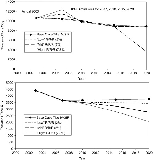
FIGURE 6-1 National SO2 and NOx emissions under R/R/R and base case scenarios, under Title IV and SIP caps (no CAIR-CAMR).
As explained above, a comparison of the nationwide NOx and SO2 emissions of an “avoid” prerevision NSR RMRR scenario with the ERP has been undertaken by EPA (2003c) in its RIA, and by other national modeling studies.13 The basic conclusion of EPA’s analysis, summarized earlier
|
13 |
Two other national analyses of the ERP change have been undertaken that also assume that electricity-generating facilities adopt the “avoid” strategy under the old NSR rule. Both used the National Energy Modeling System (NEMS), a bottom-up model of the U.S. energy sector, briefly mentioned in Chapter 4. The NEMS analysis by EPA (2003c) adopted a wider range of assumptions than the IPM-based RIA concerning efficiency and capacity availability improvements resulting from the rule change. The conclusions are qualitatively the same, |
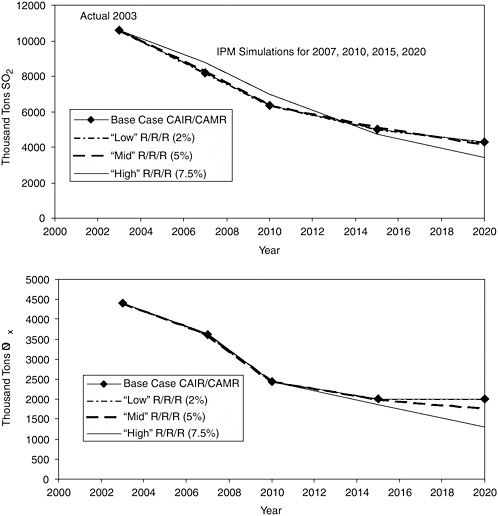
FIGURE 6-2 National SO2 and NOx emissions under R/R/R and base case scenarios, under CAIR-CAMR emission caps.
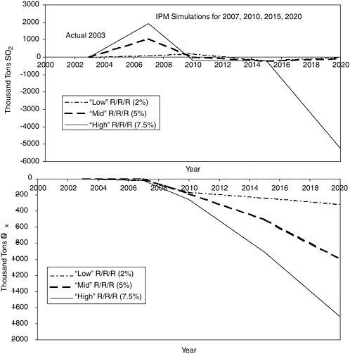
FIGURE 6-3 Difference in national SO2 and NOx emissions under Title IV NOx SIP call emission caps (comparison of prerevision NSR RMRR with the ERP base case in Figure 6-1).
in this chapter, is that in the presence of tight emission caps shifts in plant efficiency and capacity due to the ERP would not appreciably affect total national emissions of these pollutants. As mentioned earlier, the committee has reached no conclusion as to whether the “avoid” assumptions are more realistic than the assumption of the R/R/R cases that the prerevision NSR RMRR would induce additional large amounts of R/R/R.
We have not considered the effect of the “avoid” variant of the prerevision NSR RMRR under the tighter caps that would prevail under CAIR-CAMR, because, as pointed out above, tighter caps will not change the
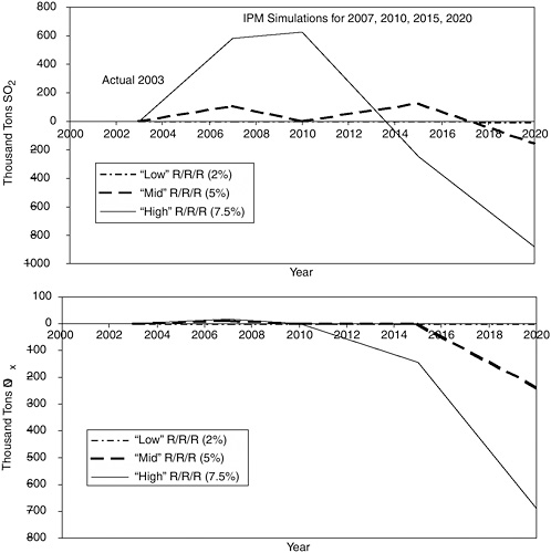
FIGURE 6-4 Difference in national SO2 and NOx emissions under CAIR-CAMR emission caps (comparison of prerevision NSR RMRR with the ERP base case in Figure 6-2).
qualitative results if emissions are already at the cap. Rather, emissions will remain at the cap.
The rest of this section is devoted to our comparison of the R/R/R variants of the prerevision NSR RMRR with the ERP. Tables 6-6a to 6-6d provide some details on the prerevision NSR R/R/R and ERP simulations for the years 2007, 2010, 2015, and 2020, including information on the mix of generation sources, the types of generation capacity, sources of coal, and what types of R/R/R decisions are made in each case. The results show that generating-plant owners nearly always respond to an assumed mandate to
retrofit, repower, or retire by retrofitting emission controls. Imposition of even the most aggressive technology constraint (“high”) results in a decision by less than 2% of the uncontrolled capacity to retire or repower.14 The solutions show relatively little difference in the share of coal-fired generation but some variation in the sources of coal. The latter result comes about because differing amounts of scrubbing and allowance prices cause electricity-generating facilities to switch between coal sources with differing costs and sulfur content.
Figure 6-5 shows the trends over time in the cumulative amount of capacity scrubbed since 2007 for the R/R/R and base case solutions and one additional solution (“Minimal Cost”) discussed later. Under the Title IV-NOx SIP call regulatory scenario (Figure 6-5 top), the R/R/R constraint is binding in each year, and the amount of scrubbed capacity increases linearly according to the assumptions in each scenario. But under the CAIR-CAMR-BART scenario (Figure 6-5 bottom), the R/R/R constraint has negligible effect in the early years. Only in the later years does that constraint bind, and then only in the “middle” and “high” R/R/R scenarios. Because of the higher allowance prices under CAIR-CAMR than under Title IV, sufficient scrubber capacity is added to more than meet the “low” R/R/R constraint in all years and the “middle” R/R/R constraint through 2015. In those cases, enforcement of the prerevision NSR RMRR results in scrubber installations that would have occurred anyway, although not necessarily at the same places, possibly increasing costs.15 However, by 2020, the “high” R/R/R scenario has resulted in 50% more retrofits than the other cases.16
The emission results for prerevision NSR RMRR R/R/R variants show the following general patterns. Under the assumption that only Title IV and the NOx SIP call caps are in place, all three of the R/R/R scenarios yield some emission changes. That is, EPA’s prerevision NSR RMRR policy is estimated to have some effects on national emissions under scenarios in which a minimum of 2-7.5% per year of the nonscrubbed coal capacity in 2004 chooses to R/R/R, assuming no tightening of emission caps. The effects are important for the 2%/year and 5%/year scenarios only for NOx. SO2
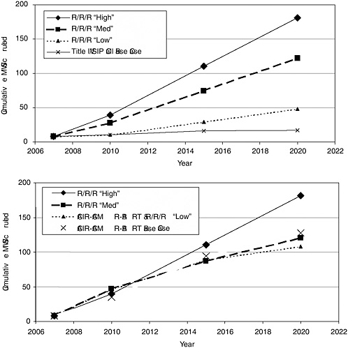
FIGURE 6-5 Cumulative FGD retrofits since 2007 for base case and prerevision NSR RMRR solutions under (top) Title IV-NOx SIP call and (bottom) CAIR-CAMR-BART.
emissions show some changes for the 5% scenario, but the anticipated 2% decrease in 2010 is more than matched by a predicted increase of 10% in 2007, with only negligible total effects over the entire time horizon of IPM. Only for the “high” (7.5%) scenarios are there so many retrofits of scrubbers that the SO2 emissions are pulled below the Title IV cap by more than about 1-2%, and then only in 2020. By that year, nearly all coal capacity is scrubbed, and SO2 emissions fall to 41% of the base case value. Meanwhile, NOx emissions in that year are 54% of the base case values. Thus, installing emission controls on 62.5% of the 2004 uncontrolled coal capacity is not sufficient to pull both pollutants much below their caps, this being (a) the percentage scrubbed in 2020 in the “middle” (5%) scenario and in 2015
TABLE 6-6a Detailed Results of IPM Simulations for Year 2007
|
Other regulations: |
Title IV and NOx SIP Call |
|||
|
Lower Bound on R/R/R (%/yr increase) |
ERP (0%) |
Prerevision NSR “Low” 2% |
Prerevision NSR “Middle” 5% |
Prerevision NSR “High” 7.5% |
|
National emissions |
|
|
|
|
|
SO2 (million short tons) |
10,374 |
10,463 |
11,433 |
12,314 |
|
NOx (million short tons) |
3,665 |
3,653 |
3,662 |
3,643 |
|
CO2 (million metric tons) |
2,391 |
2,390 |
2,392 |
2,387 |
|
Hg (short tons) |
52.0 |
52.2 |
52.9 |
53.3 |
|
Generating capacity (GW) |
||||
|
Coal |
305 |
305 |
305 |
302 |
|
Hydro |
110 |
110 |
110 |
110 |
|
Nuclear |
100 |
100 |
100 |
100 |
|
Oil-natural gas |
387 |
387 |
387 |
387 |
|
Other |
12 |
12 |
12 |
12 |
|
Renewables |
13 |
13 |
13 |
13 |
|
Total |
927 |
927 |
927 |
924 |
|
Energy generation (thousand GWh) |
||||
|
Coal |
2,161 |
2,160 |
2,164 |
2,158 |
|
Hydro |
298 |
298 |
299 |
299 |
|
Nuclear |
785 |
785 |
785 |
785 |
|
Oil-natural gas |
655 |
656 |
653 |
658 |
|
Other |
68 |
68 |
68 |
68 |
|
Renewables |
54 |
54 |
54 |
54 |
|
Total |
4,021 |
4,021 |
4,023 |
4,022 |
|
Retrofits (cumulative GW, 2007-2020) |
||||
|
FGDa |
7.8 |
8.0 |
8.0 |
8.0 |
|
SCRa |
20.2 |
21.7 |
21.8 |
22.3 |
|
SNCR |
2.5 |
0.2 |
0.2 |
0.2 |
|
ACIb |
0.0 |
0.0 |
0.0 |
0.0 |
|
Coal retirements and repowering (cumulative GW, 2007-2020) |
||||
|
Repower to CC |
0.0 |
0.0 |
0.0 |
0.0 |
|
Repower to IGCC |
0.0 |
0.0 |
0.0 |
0.0 |
|
Coal retired |
0.0 |
0.0 |
0.0 |
2.2 |
|
Oil-gas retired |
41.1 |
41.0 |
40.9 |
40.1 |
|
Total |
41.1 |
41.0 |
40.9 |
42.3 |
|
Coal production (million tons) |
||||
|
Appalachia |
334 |
332 |
335 |
342 |
|
Interior |
164 |
170 |
187 |
200 |
|
West |
577 |
572 |
551 |
525 |
|
Total |
1,075 |
1,074 |
1,073 |
1,067 |
|
Total cost ($ billion 1999) |
81.2 |
81.2 |
81.0 |
80.9 |
|
aIPM database assumes that 107 GW and 105 GW of coal-fired capacity are retrofitted with FGD and SCR, respectively, before 2007. bActivated carbon injection, a mercury-control technology. |
||||
|
CAIR-CAMR-BART |
|||
|
ERP (0%) |
Prerevision NSR “Low” 2% |
Prerevision NSR “Middle” 5% |
Prerevision NSR “High” 7.5% |
|
|
|
|
8,75 |
|
8,172 |
8,173 |
8,279 |
6 |
|
3,613 |
3,613 |
3,623 |
3,629 |
|
2,369 |
2,370 |
2,374 |
2,380 |
|
47.4 |
47.4 |
47.5 |
49.2 |
|
|
|||
|
300 |
300 |
301 |
302 |
|
110 |
110 |
110 |
110 |
|
100 |
100 |
100 |
100 |
|
387 |
387 |
387 |
387 |
|
12 |
12 |
12 |
12 |
|
13 |
13 |
13 |
13 |
|
922 |
922 |
923 |
924 |
|
|
|||
|
2,127 |
2,128 |
2,134 |
2,144 |
|
292 |
292 |
293 |
295 |
|
785 |
785 |
785 |
785 |
|
685 |
685 |
680 |
670 |
|
68 |
68 |
68 |
68 |
|
54 |
54 |
54 |
54 |
|
4,011 |
4,012 |
4,014 |
4,016 |
|
|
|||
|
8.0 |
8.0 |
8.0 |
8.0 |
|
17.1 |
17.1 |
17.9 |
18.8 |
|
0.2 |
0.2 |
0.2 |
0.2 |
|
|
|||
|
0.0 |
0.0 |
0.0 |
0.0 |
|
0.0 |
0.0 |
0.0 |
0.0 |
|
0.0 |
0.0 |
0.0 |
0.0 |
|
4.2 |
4.1 |
3.1 |
2.3 |
|
40.6 |
40.5 |
40.5 |
40.5 |
|
44.8 |
44.6 |
43.6 |
42.8 |
|
|
|||
|
299 |
299 |
303 |
312 |
|
138 |
138 |
140 |
142 |
|
628 |
628 |
625 |
617 |
|
1,065 |
1,065 |
1,068 |
1,071 |
|
|
|||
|
82.3 |
82.3 |
82.3 |
81.8 |
TABLE 6-6b Detailed Results of IPM Simulations for Year 2010
|
Other Regulations: |
Title IV and NOx SIP Call |
|||
|
Lower Bound on R/R/R (%/yr increase) |
ERP (0%) |
“Low” 2% |
Prerevision NSR “Middle” 5% |
Prerevision NSR “High” 7.5% |
|
National emissions |
|
|
|
|
|
SO2 (million short tons) |
9,908 |
10,094 |
9,899 |
9,719 |
|
NOx (million short tons) |
3,679 |
3,516 |
3,496 |
3,426 |
|
CO2 (million metric tons) |
2,470 |
2,469 |
2,474 |
2,472 |
|
Hg (short tons) |
50.6 |
50.7 |
50.9 |
49.0 |
|
Generating capacity (GW) |
||||
|
Coal |
305 |
305 |
305 |
302 |
|
Hydro |
110 |
110 |
110 |
110 |
|
Nuclear |
101 |
101 |
101 |
101 |
|
Oil-natural gas |
393 |
393 |
394 |
395 |
|
Other |
12 |
12 |
12 |
12 |
|
Renewables |
13 |
13 |
13 |
13 |
|
Total |
934 |
934 |
934 |
933 |
|
Energy generation (thousand GWh) |
||||
|
Coal |
2,198 |
2,195 |
2,201 |
2,199 |
|
Hydro |
297 |
298 |
300 |
301 |
|
Nuclear |
799 |
799 |
799 |
799 |
|
Oil-natural gas |
777 |
780 |
776 |
777 |
|
Other |
71 |
71 |
71 |
71 |
|
Renewables |
56 |
56 |
56 |
56 |
|
Total |
4,198 |
4,199 |
4,203 |
4,202 |
|
Retrofits (cumulative GW, 2007-2020) |
||||
|
FGDa |
10.4 |
11.0 |
27.8 |
39.8 |
|
SCRa |
25.9 |
24.7 |
28.2 |
40.2 |
|
SNCR |
5.0 |
0.2 |
0.2 |
0.2 |
|
ACIb |
0.3 |
0.2 |
0.2 |
0.2 |
|
Coal retirements and repowering (cumulative GW, 2007-2020) |
||||
|
Repower to CC |
0.9 |
0.9 |
0.9 |
0.9 |
|
Repower to IGCC |
0.1 |
0.1 |
0.1 |
0.1 |
|
Coal retired |
0.0 |
0.0 |
0.0 |
2.2 |
|
Oil-gas retired |
42.0 |
41.7 |
41.5 |
40.6 |
|
Total |
43.0 |
42.7 |
42.5 |
43.8 |
|
Coal production (million tons) |
||||
|
Appalachia |
325 |
329 |
345 |
353 |
|
Interior |
161 |
164 |
187 |
210 |
|
West |
603 |
594 |
554 |
513 |
|
Total |
1,089 |
1,087 |
1,086 |
1,076 |
|
Total cost ($ billion 1999) |
85.5 |
85.6 |
85.8 |
86.3 |
|
aIPM database assumes that 107 GW and 105 GW of coal-fired capacity are retrofitted with FGD and SCR, respectively, before 2007. bActivated carbon injection, a mercury-control technology. |
||||
|
CAIR-CAMR-BART |
|||
|
ERP (0%) |
Prerevision NSR “Low” 2% |
Prerevision NSR “Middle” 5% |
Prerevision NSR “High” 7.5% |
|
|
|||
|
6,344 |
6,344 |
6,343 |
6,967 |
|
2,439 |
2,439 |
2,438 |
2,438 |
|
2,445 |
2,445 |
2,447 |
2,453 |
|
35.3 |
35.3 |
35.5 |
36.7 |
|
|
|||
|
300 |
300 |
301 |
302 |
|
110 |
110 |
110 |
110 |
|
101 |
101 |
101 |
101 |
|
394 |
394 |
394 |
394 |
|
12 |
12 |
12 |
12 |
|
13 |
13 |
13 |
13 |
|
930 |
930 |
931 |
932 |
|
|
|||
|
2,160 |
2,160 |
2,162 |
2,173 |
|
290 |
290 |
290 |
291 |
|
799 |
799 |
799 |
799 |
|
812 |
812 |
810 |
800 |
|
71 |
71 |
71 |
71 |
|
56 |
56 |
56 |
56 |
|
4,188 |
4,188 |
4,188 |
4,190 |
|
|
|||
|
46.4 |
46.4 |
47.0 |
39.6 |
|
41.1 |
41.2 |
42.2 |
43.7 |
|
0.2 |
0.2 |
0.2 |
0.2 |
|
2.2 |
2.2 |
1.8 |
1.7 |
|
|
|||
|
0.9 |
0.9 |
0.9 |
0.9 |
|
0.1 |
0.1 |
0.1 |
0.1 |
|
4.7 |
4.6 |
3.6 |
2.4 |
|
41.2 |
41.1 |
40.9 |
41.1 |
|
46.9 |
46.7 |
45.5 |
44.5 |
|
|
|||
|
303 |
303 |
305 |
315 |
|
169 |
169 |
169 |
164 |
|
589 |
589 |
587 |
587 |
|
1,061 |
1,061 |
1,062 |
1,066 |
|
|
|||
|
88.2 |
88.2 |
88.3 |
87.9 |
TABLE 6-6c Detailed Results of IPM Simulations for Year 2015
|
Other Regulations: |
Title IV and NOx SIP Call |
|||
|
Lower Bound on R/R/R (%/yr increase) |
ERP (0%) |
Prerevision NSR “Low” 2% |
Prerevision NSR “Middle” 5% |
Prerevision NSR “High” 7.5% |
|
National emissions |
||||
|
SO2 (million short tons) |
9,084 |
8,873 |
8,865 |
8,854 |
|
NOx (million short tons) |
3,721 |
3,487 |
3217 |
2,808 |
|
CO2 (million metric tons) |
2,599 |
2,597 |
2,604 |
2,597 |
|
Hg (short tons) |
48.9 |
48.7 |
48.3 |
48.1 |
|
Generating capacity (GW) |
||||
|
Coal |
305 |
305 |
304 |
301 |
|
Hydro |
110 |
110 |
110 |
110 |
|
Nuclear |
102 |
102 |
102 |
102 |
|
Oil-natural gas |
421 |
421 |
422 |
424 |
|
Other |
12 |
12 |
12 |
12 |
|
Renewables |
14 |
14 |
14 |
14 |
|
Total |
964 |
964 |
964 |
963 |
|
Energy generation (thousand GWh) |
||||
|
Coal |
2,242 |
2,240 |
2,244 |
2,228 |
|
Hydro |
296 |
296 |
298 |
297 |
|
Nuclear |
811 |
811 |
811 |
811 |
|
Oil-natural gas |
1,026 |
1,028 |
1,026 |
1,040 |
|
Other |
67 |
67 |
67 |
67 |
|
Renewables |
61 |
61 |
60 |
60 |
|
Total |
4,503 |
4,503 |
4,506 |
4,503 |
|
Retrofits (cumulative GW, 2007-2020) |
||||
|
FGDa |
16.0 |
29.8 |
74.9 |
110.4 |
|
SCRa |
33.3 |
35.8 |
75.5 |
111.0 |
|
SNCR |
7.6 |
0.2 |
0.2 |
0.2 |
|
ACIb |
0.3 |
0.2 |
0.2 |
0.2 |
|
Coal retirements and repowering (cumulative GW, 2007-2020) |
||||
|
Repower to CC |
0.9 |
0.9 |
0.9 |
0.9 |
|
Repower to IGCC |
0.1 |
0.1 |
0.1 |
0.1 |
|
Coal retired |
0.0 |
0.0 |
0.0 |
2.2 |
|
Oil-gas retired |
42.0 |
41.7 |
41.5 |
40.6 |
|
Total |
43.0 |
42.7 |
42.5 |
43.8 |
|
Coal production (million tons) |
||||
|
Appalachia |
315 |
316 |
354 |
364 |
|
Interior |
162 |
183 |
243 |
260 |
|
West |
631 |
603 |
496 |
468 |
|
Total |
1,108 |
1,102 |
1,094 |
1,092 |
|
Total cost ($ billion 1999) |
96.0 |
96.2 |
98.1 |
100.6 |
|
aIPM database assumes that 107 GW and 105 GW of coal-fired capacity are retrofitted with FGD and SCR, respectively, before 2007. bActivated carbon injection, a mercury-control technology. |
||||
|
CCAIR-CAMR-BART |
|||
|
ERP (0%) |
Prerevision NSR “Low” 2% |
Prerevision NSR “Middle” 5% |
Prerevision NSR “High” 7.5% |
|
|
|||
|
4,992 |
4,994 |
5,119 |
4742 |
|
1,994 |
1,994 |
1,994 |
1850 |
|
2,569 |
2,568 |
2,575 |
2,590 |
|
31.9 |
31.9 |
32.3 |
29.9 |
|
|
|||
|
299 |
299 |
300 |
301 |
|
110 |
110 |
110 |
110 |
|
102 |
102 |
102 |
102 |
|
426 |
426 |
425 |
425 |
|
12 |
12 |
12 |
12 |
|
14 |
14 |
14 |
14 |
|
963 |
963 |
963 |
964 |
|
|
|||
|
2,194 |
2,194 |
2,202 |
2,222 |
|
294 |
293 |
294 |
296 |
|
811 |
811 |
811 |
811 |
|
1,072 |
1,072 |
1,064 |
1,046 |
|
67 |
67 |
67 |
67 |
|
61 |
61 |
61 |
61 |
|
4,499 |
4,498 |
4,499 |
4,503 |
|
|
|||
|
88.3 |
88.1 |
86.6 |
110.3 |
|
70.6 |
70.6 |
74.0 |
110.8 |
|
0.3 |
0.3 |
0.2 |
0.2 |
|
2.7 |
2.7 |
2.4 |
2.4 |
|
|
|||
|
0.9 |
0.9 |
0.9 |
0.9 |
|
0.1 |
0.1 |
0.1 |
0.1 |
|
4.7 |
4.6 |
3.6 |
2.4 |
|
41.2 |
41.1 |
40.9 |
41.1 |
|
46.9 |
46.7 |
45.5 |
44.5 |
|
|
|||
|
310 |
309 |
312 |
341 |
|
194 |
194 |
194 |
224 |
|
568 |
568 |
570 |
514 |
|
1,072 |
1,071 |
1,076 |
1,079 |
|
|
|||
|
100.4 |
100.4 |
100.3 |
101.5 |
TABLE 6-6d Detailed Results of IPM Simulations for Year 2020
|
Other Regulations: |
Title IV and NOx SIP Call |
|||
|
Lower Bound on R/R/R (%/yr increase) |
ERP (0%) |
Prerevision NSR “Low” 2% |
Prerevision NSR “Middle” 5% |
Prerevision NSR “High” 7.5% |
|
National emissions |
||||
|
SO2 (million short tons) |
8,876 |
8,862 |
8,787 |
3,632 |
|
NOx (million short tons) |
3,758 |
3,445 |
2,760 |
2,041 |
|
CO2 (million metric tons) |
2,796 |
2,797 |
2,797 |
2,799 |
|
Hg (short tons) |
50.2 |
49.1 |
48.1 |
40.7 |
|
Generating capacity (GW) |
||||
|
Coal |
326 |
325 |
323 |
321 |
|
Hydro |
110 |
110 |
110 |
110 |
|
Nuclear |
103 |
103 |
103 |
103 |
|
Oil-natural gas |
467 |
468 |
470 |
471 |
|
Other |
12 |
12 |
12 |
12 |
|
Renewables |
14 |
14 |
14 |
14 |
|
Total |
1,032 |
1,032 |
1,032 |
1,031 |
|
Energy generation (thousand GWh) |
||||
|
Coal |
2,410 |
2,411 |
2,396 |
2,388 |
|
Hydro |
294 |
295 |
295 |
295 |
|
Nuclear |
809 |
809 |
809 |
809 |
|
Oil-natural gas |
1,221 |
1,221 |
1,237 |
1,244 |
|
Other |
54 |
54 |
54 |
54 |
|
Renewables |
61 |
61 |
60 |
60 |
|
Total |
4,849 |
4,851 |
4,851 |
4,850 |
|
Retrofits (cumulative GW, 2007-2020) |
||||
|
FGDa |
17.1 |
48.7 |
122.1 |
181.1 |
|
SCRa |
35.8 |
49.2 |
122.8 |
181.4 |
|
SNCR |
8.4 |
0.2 |
0.2 |
0.2 |
|
ACIb |
0.3 |
0.2 |
0.2 |
0.2 |
|
Coal retirements and repowering (cumulative GW, 2007-2020) |
||||
|
Repower to CC |
0.9 |
0.9 |
0.9 |
0.9 |
|
Repower to IGCC |
0.1 |
0.1 |
0.1 |
0.1 |
|
Coal retired |
0 |
0 |
0 |
2.2 |
|
Oil-gas retired |
42 |
41.7 |
41.5 |
40.6 |
|
Total |
42 |
42.7 |
42.5 |
43.8 |
|
Coal production (million tons) |
||||
|
Appalachia |
301 |
336 |
383 |
392 |
|
Interior |
173 |
227 |
275 |
269 |
|
West |
714 |
600 |
495 |
505 |
|
Total |
1,188 |
1,163 |
1,152 |
1,166 |
|
Total cost ($ billion 1999) |
109.4 |
110.2 |
114.5 |
119.3 |
|
aIPM database assumes that 107 GW and 105 GW of coal-fired capacity are retrofitted with FGD and SCR, respectively, before 2007. bActivated carbon injection, a mercury-control technology. |
||||
|
CAIR-CAMR-BART |
|||
|
ERP (0%) |
Prerevision NSR “Low” 2% |
Prerevision NSR “Middle” 5% |
Prerevision NSR “High” 7.5% |
|
|
|||
|
4,282 |
4,279 |
4,126 |
3,399 |
|
2,002 |
2,002 |
1,763 |
1,312 |
|
2,758 |
2,758 |
2,772 |
2,789 |
|
28.7 |
28.7 |
27.6 |
26.8 |
|
|
|||
|
321 |
321 |
320 |
320 |
|
110 |
110 |
110 |
110 |
|
103 |
103 |
103 |
103 |
|
472 |
472 |
472 |
473 |
|
12 |
12 |
12 |
12 |
|
14 |
14 |
14 |
14 |
|
1,032 |
1,032 |
1,031 |
1,032 |
|
|
|||
|
2,358 |
2,357 |
2,373 |
2,375 |
|
292 |
292 |
294 |
295 |
|
809 |
809 |
809 |
809 |
|
1,272 |
1,273 |
1,258 |
1,257 |
|
54 |
54 |
54 |
54 |
|
61 |
61 |
61 |
61 |
|
4,846 |
4,846 |
4,849 |
4,851 |
|
|
|||
|
107.9 |
108.1 |
120.3 |
181 |
|
72.9 |
72.9 |
120.9 |
181.3 |
|
0.5 |
0.5 |
0.2 |
0.2 |
|
11.1 |
11.1 |
5 |
4.7 |
|
|
|||
|
0.9 |
0.9 |
0.9 |
0.9 |
|
0.1 |
0.1 |
0.1 |
0.1 |
|
4.7 |
4.6 |
3.9 |
2.4 |
|
41.2 |
41.1 |
40.9 |
41.1 |
|
46.9 |
46.7 |
45.8 |
44.5 |
|
|
|||
|
330 |
330 |
343 |
398 |
|
225 |
226 |
246 |
286 |
|
568 |
568 |
536 |
463 |
|
1,123 |
1,124 |
1,125 |
1,147 |
|
|
|||
|
115.6 |
115.5 |
116.3 |
120.5 |
in the “high” scenario. Only NOx emissions fall more than about 1-2% below the cap at that level of control. As mentioned, the committee regards the “high” case as an unlikely high level of emission-control retrofit, so it does not regard the 2020 SO2 reductions in that scenario as being likely outcomes of the prerevision NSR rule. However, because NOx reductions occur under a less extreme “middle” scenario, we regard the possibility of NOx increases associated with the ERP as being plausible, given the present Title IV and NOx SIP call caps.17
The different conclusions concerning national NOx and SO2 emissions are due in part to the greater flexibility that generators have in ways to adjust (either reduce or increase) SO2 emissions than they have for NOx and in part due to the more comprehensive nature of SO2 regulation in the absence of CAIR. SO2 emissions can be adjusted either by switching to grades of coal with different sulfur contents or by installing postcombustion controls. Once a scrubber is installed, a coal-fired generator that previously burned low-sulfur coal may switch to less expensive higher-sulfur coal to keep its costs down, thereby limiting the ultimate effect of the retrofit on total emission of SO2 from the facility.18 For NOx, the options are typically more limited. Once an SCR is installed, the associated reduction in the NOx emission rate will not be partly or wholly offset by a change in fuel choice. In the absence of CAIR, the seasonal, regional NOx cap-and-trade program under the NOx SIP call is both geographically and temporally less comprehensive than the national annual SO2 cap-and-trade program under Title IV. Thus, a smaller percentage of total NOx emissions from the electricity sector are subject to a cap than the nearly 100% of SO2 emissions that come under a cap.
We turn now to the analysis under the tighter caps under CAIR-CAMR. Considering the various R/R/R scenarios, the 2%/year and 5%/year simulations indicate that except for NOx in the year 2020 national emissions are not pulled below the caps. NOx falls 10% below the cap in 2020 in the 5%/year scenario; considerably less than if only Title IV and the NOx SIP call were in place. Under the most extreme prerevision NSR case (“high,” 7.5%/year R/R/R, involving almost 100% of coal capacity by 2020), SO2 emissions fall below the cap slightly in 2015 and then by 20% in 2020. The tonnage of SO2 in 2020 in that case is nearly the same as in the Title IV “high” R/R/R case (3,400 kT/year versus 3,600 kT/year). That is not
surprising, in that the caps in both cases are no longer effective, and practically all coal-fired capacity has scrubbers and SCR.
To get a sense of where emission reductions are occurring, we look at SO2 and NOx emission changes under the different R/R/R scenarios at CAIR-affected model plants and plants not affected by CAIR.19 The model results indicate that most of the NOx emission reductions with the R/R/R “high” scenario (given CAMR-CAIR) occur at non-CAIR-affected units, although in 2020 emissions from CAIR-affected units are reduced as well. For SO2, the emission reductions in 2015 under the “high” scenario occur at CAIR-affected model plants, and emission reductions in 2020 are split between CAIR-affected and non-CAIR-affected model plants.
Although the committee has determined that the “high” scenario is an unlikely outcome of the prerevision NSR EPA RMRR policy, it does illustrate some interesting interactions of this type of rule with emission caps. In particular, what is surprising is that the SO2 decrease in 2015 and 2020 in the “high” scenario (given CAMR-CAIR) is matched almost ton for ton by increases in 2007 and 2010. Thus, total emissions over the entire time horizon remain at or very near the cap. As the amount of scrubbing increases in later years, the price of emission allowances falls. If generation owners anticipate that development in earlier years, they will have weaker incentives for making early reductions in emissions and then banking the allowances for later use. The diminished value of banked allowances does not justify the marginal cost of fuel-switching, emission dispatch,20 and other nonscrubbing emission-reduction measures in the early years.21 Thus, the main effect of the “high” (7.5%/year) R/R/R constraint has been to redistribute SO2 emissions over the period 2007-2020, not to reduce the total. If marginal health and other damages are increasing with emissions and any positive discount rate is used to evaluate damages, this redistribution cannot be viewed as a good outcome. However, it is possible that emissions in 2025 and later will be lower under the “high” scenario than under that base case
and remain there, so damages in the long term might be less in the presence of that constraint. However, such a conclusion would need to assume that emission caps are not tightened after 2020; the likelihood of that cannot be assessed by this committee.
In contrast, the changes in NOx emissions in the “high” scenario under CAIR-CAMR present no such ambiguity. There are no emission increases in earlier years relative to the base case, and emissions fall by 7% in 2015 and 34% in 2020. Thus, in the bounding case where nearly every coal-fired generator is assumed to be compelled by settlement or economics to be R/R/R by 2020 and there is assumed to be no change in the CAIR caps, there are NOx emission benefits of the prerevision NSR rules relative to the ERP. Those benefits largely or completely disappear if what this committee considers to be more likely rates of R/R/R occur (0%, 2% “low,” or 5%/yr “middle”).
One indication of the effectiveness of economic incentives to lower SO2 and NOx emissions is revealed by comparing the “high” scenarios under Title IV-NOx SIP call and under CAIR-CAMR. For instance, those two solutions have similar amounts of FGD retrofits in every year, because the SO2 R/R/R constraint is binding in both cases in each year. However, a comparison of the SO2 graphs in Figures 6-1 and 6-2 shows that they have very different amounts of emissions in 2007-2015. The use of fuel switching and fuel blending under CAIR-CAMR results in SO2 emissions that are nearly 30% less than the Title IV-NOx SIP call results in 2007 and 2010 and 46% less in 2015. The story is similar for NOx emissions: the amount of SCR installations is essentially the same in each year, but emissions in the CAIR-CAMR case are 70% of those in the Title IV-NOx SIP call simulation for 2010 and later (compare the NOx graphs in Figures 6-1 and 6-2).
These are two reasons for these solutions to have similar emission-control retrofits but different emissions. First, the higher price of NOx and SO2 allowances in the CAIR-CAMR cases motivates installation of the control retrofits at locations where the emission controls are most cost effective. That is consistent with the idea that under the CAIR caps one would expect the NOx controls to be installed first at the plants that can achieve the most cost-effective reductions. However, with only the type of rule used for NSR, controls might instead be installed at plants with low installation and operation costs per megawatt and not necessarily where the costs per ton of reductions are lowest. Second, allowance costs also motivate the adoption of fuel-switching and emission-dispatch strategies that can cost-effectively reduce emissions at generating units that are not retrofitted with FGD or SCR. In general, the least costly way of achieving an emission target involves a mix of emission-control investments, fuel-switching, and operational changes (Heslin and Hobbs, 1991). Strategies, such as the emission-control retrofits required by NSR settlements, can be relatively inefficient because
they provide no incentives to adopt such combination strategies. Cap-based policies, in contrast, create a level playing field among alternative means of reducing emissions.
Sensitivity Analysis
As mentioned above, we have rerun the R/R/R “high” solution under CAIR-CAMR using alternative assumptions concerning the cost of alternative generation technologies. In particular, we are testing whether substantially lower natural gas prices or lower investment costs for renewables (wind, solar, landfill gas, biomass, and geothermal) and integrated gasification combined-cycle generation (IGCC) could affect our conclusions by pulling emissions below the cap earlier or by a larger amount. Table 6-7 compares that R/R/R “high” solution under base case investment and gascost assumptions with a R/R/R “high” solution that has lower renewable and IGCC investment costs (“low capital”) and a second R/R/R “high” sensitivity case that, in addition, has much lower natural gas prices (“low capital-gas”).
Considering first the sensitivity analysis involving lower investment costs for renewables and IGCC, we conclude that those assumptions make almost no difference in emission, generation mix, and emission controls, at least through 2020. Renewable generation capacity goes up by about 15% in 2020, but because this is from a small base (14 GW, less than 5% of the amount of coal capacity), there is negligible effect on emissions. There is no additional repowering to IGCC, but new IGCC rises from 6.9 GW to 12.2 GW by 2020 (about 3% of total coal capacity). The latter displaces some other types of capacity additions that occurred in the base R/R/R “high” case but does not appreciably affect total system emissions.
A greater effect on emissions occurs in the second sensitivity analysis (low gas cost and low renewables and IGCC investment cost). SO2 emissions fall by about 3% in 2020, although the total 2007-2015 SO2 emissions are essentially unchanged, as are 2007-2020 NOx emissions. The fall in SO2 emissions occurs because natural gas energy generation expands by 15% (compared with the R/R/R “high” case), mainly at the expense of coal generation. Natural gas capacity increases by 25 GW compared with the R/R/R “high” case, and the increase is matched by an identical decrease in coal capacity. Thus, a mix of generation, especially new plant additions, is somewhat sensitive to gas prices and investment cost assumptions. However, the basic conclusion—that SO2 emissions are pulled slightly below the CAIR-CAMR cap by 2020 only if all existing unscrubbed capacity is retrofitted with scrubbers and that NOx emissions would be pulled below the CAIR cap in 2015 only if nearly all coal capacity is retrofitted with SCR—is unaffected.
TABLE 6-7 Sensitivity Analyses of R/R/R Case: Lower Capital Costs for Renewables and IGCC and Lower Natural Gas Prices
|
Variable |
Solution |
2007 |
2010 |
2015 |
2020 |
|
National emissions |
|||||
|
SO2 (thousand tons) |
R/R/R “high” |
8,756 |
6,967 |
4,742 |
3,399 |
|
|
Low capital |
8,743 |
6,974 |
4,735 |
3,406 |
|
|
Low capital-gas |
8,782 |
7,011 |
4,674 |
3,292 |
|
NOx (thousand tons) |
R/R/R “high” |
3,629 |
2,438 |
1,850 |
1,312 |
|
|
Low capital |
3,628 |
2,441 |
1,859 |
1,329 |
|
|
Low capital-gas |
3,611 |
2,430 |
1,873 |
1,307 |
|
CO2 (million tons) |
R/R/R “high” |
2,380 |
2,453 |
2,590 |
2,789 |
|
|
Low capital |
2,378 |
2,451 |
2,600 |
2,822 |
|
|
Low capital-gas |
2,374 |
2,418 |
2,556 |
2,707 |
|
Hg (tons) |
R/R/R “high” |
49 |
37 |
30 |
27 |
|
|
Low capital |
49 |
37 |
30 |
27 |
|
|
Low capital-gas |
49 |
37 |
30 |
26 |
|
Retrofits (cumulative GW from 2007) |
|||||
|
FGD |
R/R/R “high” |
8.0 |
39.6 |
110.3 |
181 |
|
|
Low capital |
8.0 |
39.0 |
109.7 |
179.2 |
|
|
Low capital-gas |
8.0 |
34.4 |
104.9 |
175.3 |
|
|
SCR R/R/R “high” |
18.8 |
43.7 |
110.8 |
181.3 |
|
|
Low capital |
18.6 |
43.2 |
110.1 |
179.3 |
|
|
Low capital-gas |
18.2 |
37.7 |
104.8 |
175.0 |
|
Coal retirements and repowering (cumulative GW, 2007-2020) |
|||||
|
Repower to CC |
R/R/R “high” |
0.0 |
0.9 |
0.9 |
0.9 |
|
|
Low capital |
0.0 |
0.9 |
0.9 |
0.9 |
|
|
Low capital-gas |
0.0 |
0.9 |
0.9 |
0.9 |
|
Repower to IGCC |
R/R/R “high” |
0.0 |
0.1 |
0.1 |
0.1 |
|
|
Low capital |
0.0 |
0.1 |
0.1 |
0.1 |
|
|
Low capital-gas |
0.0 |
0.0 |
0.1 |
0.1 |
|
Coal retired |
R/R/R “high” |
2.3 |
2.4 |
2.4 |
2.4 |
|
|
Low capital |
3.0 |
3.1 |
3.1 |
4.4 |
|
|
Low capital-gas |
7.2 |
8.4 |
9.0 |
9.4 |
|
Oil/gas retired |
R/R/R “high” |
40.5 |
41.1 |
41.1 |
41.1 |
|
|
Low capital |
40.5 |
41.0 |
41.0 |
41.0 |
|
|
Low capital-gas |
33.2 |
33.4 |
33.4 |
33.4 |
|
Energy generation (thousand GWh) |
|||||
|
Coal |
R/R/R “high” |
2,144 |
2,173 |
2,222 |
2,375 |
|
|
Low capital |
2,142 |
2,171 |
2,253 |
2,475 |
|
|
Low capital-gas |
2,134 |
2,118 |
2,161 |
2,189 |
|
Oil/natural gas |
R/R/R “high” |
670 |
800 |
1,046 |
1,257 |
|
|
Low capital |
670 |
800 |
1,007 |
1,149 |
|
|
Low capital-gas |
679 |
852 |
1,107 |
1,441 |
|
Variable |
Solution |
2007 |
2010 |
2015 |
2020 |
|
Renewables |
R/R/R “high” |
54 |
56 |
61 |
61 |
|
|
Low capital |
56 |
58 |
69 |
69 |
|
|
Low capital-gas |
55 |
58 |
60 |
61 |
|
Generating capacity (MW) |
|||||
|
Coal |
R/R/R “high” |
302 |
302 |
301 |
320 |
|
|
Low capital |
302 |
301 |
305 |
334 |
|
|
Low capital-gas |
297 |
296 |
294 |
295 |
|
Oil/natural gas |
R/R/R “high” |
387 |
394 |
425 |
473 |
|
|
Low capital |
387 |
394 |
419 |
458 |
|
|
Low capital-gas |
396 |
402 |
431 |
498 |
|
Renewables |
R/R/R “high” |
13 |
13 |
14 |
14 |
|
|
Low capital |
13 |
14 |
16 |
16 |
|
|
Low capital-gas |
13 |
14 |
14 |
14 |
Economic Efficiency of Different Approaches to Reducing National or Regional Emissions
To assess the potential efficiency of the R/R/R variants of the prerevision NSR RMRR, we have calculated cost effectiveness in dollars per ton for each R/R/R case against its base case for both the Title IV-NOx SIP call and the CAIR-CAMR emission cap scenarios. That is, given a set of emission caps, what is the cost per ton of emission reduction? For simplicity, the reductions include both the NOx and SO2 effects, assuming that they get equal weight in the calculation. Costs and emissions from 2007 through 2020 are considered; values for years between the solutions for 2007, 2010, 2015, and 2020 are obtained by linear interpolation. Table 6-8 shows the calculations for two assumptions about discounting emissions: one with a zero discount rate and the other with a 5%/year real discount rate. The former assumes that a ton of emissions in 2020 should be weighted just as much as a ton emitted today. The latter is more consistent with a levelized emission-costing approach.22
TABLE 6-8 Cost Effectiveness of Emission Reductions for Various Cases Compared to Base Cases
|
|
Undiscounted Emission Analysis |
|||
|
Case |
Undiscounted SO2 Emissions, 2007-2020 (thousands of tons) |
Undiscounted NOx Emissions, 2007-2020 (thousands of tons) |
Total Discounted Cost (billion of $)a |
Cost Effectiveness ($/ton) |
|
Comparison of R/R/R cases with Title IV-NOx SIP call base case |
||||
|
Base case (Title IV-NOx SIP call) |
132,430 |
51,930 |
867.2 |
|
|
Title IV-SIP with “low” R/R/R (2%) |
132,250 |
49,140 |
869.7 |
$850 |
|
Title IV-SIP with “middle” R/R/R (5%) |
133,150 |
45,670 |
882.8 |
$2,800 |
|
Title IV-SIP with “high” R/R/R (7.5%) |
118,670 |
41,150 |
899.1 |
$1,300 |
|
Comparison of R/R/R cases with CAIR-CAMR base case |
||||
|
Base case (CAIR-CAMR) |
79,520 |
32,960 |
900.9 |
|
|
CAIR-CAMR with “low” R/R/R (2%) |
79,530 |
32,960 |
900.9 |
negative |
|
CAIR-CAMR with “middle” R/R/R (5%) |
79,910 |
32,250 |
901.8 |
$2,900 |
|
CAIR-CAMR with “high” R/R/R (7.5%) |
79,280 |
30,200 |
910.1 |
$3,100 |
|
Comparison of CAIR-CAMR base case with Title IV-NOx SIP call base case |
||||
|
Base case (Title IV-NOx SIP call) |
132,430 |
51,930 |
867.2 |
|
|
Base case (CAIR-CAMR) |
79,520 |
32,960 |
900.9 |
$470 |
|
Comparison of minimal cost solution for achieving “CAIR-CAMR with ‘high’ R/R/R (7.5%)” emissions reductions with CAIR-CAMR base case |
||||
|
Base case (CAIR-CAMR) |
79,520 |
32,960 |
900.9 |
|
|
Minimal cost solution |
79,314 |
29,289 |
904.6 |
$960 |
|
a5% discount rate used, discounted to 2005; $1999 assumed for costs. The discounted costs columns are the same for both the discounted and undiscounted emissions analysis. |
||||
|
Discounted Emissions Analysis |
|||
|
Discounted SO2 Emissions, 2007-2020 (thousands of tons) |
Discounted NOx Emissions, 2007-2020 (thousands of tons)a |
Total Discounted Cost (billion of $)a |
Cost Effectiveness, Levelized ($/ton) |
|
90,090 |
34,910 |
867 |
|
|
90,140 |
33,190 |
870 |
$1,500 |
|
91,110 |
31,250 |
883 |
$5,900 |
|
84,130 |
28,640 |
899 |
$2,600 |
|
|
|||
|
55,670 |
23,010 |
900.9 |
|
|
55,670 |
23,010 |
900.9 |
negative |
|
56,000 |
22,650 |
901.8 |
|
|
|
|
|
$53,000 |
|
56,450 |
21,530 |
910.1 |
|
|
|
|
|
$13,000 |
|
90,090 |
34,910 |
867.2 |
|
|
55,670 |
23,010 |
900.9 |
$730 |
|
|
|||
|
55,670 |
23,010 |
900.9 |
|
|
56,422 |
20,831 |
904.6 |
$2,600 |
The table shows that the incremental emission reductions (relative to the Title IV-NOx SIP call base case) achieved by imposing the R/R/R constraint cost $850-5,900 per ton.23 Given the CAIR-CAMR emission reductions, the incremental cost of further R/R/R emission reductions would be between $2,900 and $53,000 per ton. For the “low” (2%) constraint case with CAIR-CAMR, the emission “reduction” is actually negative (emissions increase slightly over the 2007-2020 period), so the cost effectiveness is negative. These costs per ton of reduction are large compared with the costs of achieving emission reductions by using a cap alone, discussed next.
The cost of achieving emission reduction with a cap is gauged in two ways. First, we compare the two base cases in the third group of rows of Table 6-8. Both of those solutions assume that the ERP is in place (that is, the R/R/R constraint is omitted). That calculation shows that the cost effectiveness of the emission reductions resulting from replacing the Title IV-NOx SIP call with the CAIR-CAMR cap is $470/ton (undiscounted) to $730/ton (discounted). The most relevant comparisons are the R/R/R cost-effectiveness estimates with the Title IV-NOx SIP call base case, which yields cost-per-ton estimates ($850-$5,900/ton) that are 2-8 times as high as the corresponding cost-effectiveness estimate for the CAIR-CAMR cap by itself ($470-$730/ton). That is again not unexpected, inasmuch as the R/R/R scenario as implemented in IPM requires specific technologies at selected plants versus economic optimization as the basis for the CAIR-CAMR controls.
However, this comparison is something of an apples-versus-oranges comparison because the emission reductions involved are not identical. Therefore, we gauge whether the cost per ton of reduction in the R/R/R scenario is large in a second way: by comparing that cost with the expense per ton of achieving the same reductions with use of caps alone. To do that, IPM with the CAIR-CAMR base case assumptions was run with an additional set of constraints forcing SO2 and NOx emissions in each of the solution years to be less than or equal to the corresponding emissions obtained by the R/R/R. That is termed the “minimal cost” solution because IPM achieves those solutions at the lowest cost under the assumption that national caps with tradable rights are imposed. In the last two rows of Table 6-9 we compare that solution with the CAIR-CAMR base case.24
TABLE 6-9 Comparison of R/R/R “High” Solution (prerevision NSR RMRR) with Minimal-Cost Solution That Achieves Same Emissions
|
Year |
Solution |
2007 |
2010 |
2015 |
2020 |
|
National emissions |
|||||
|
SO2 (thousand tons) |
R/R/R “high” |
8,756 |
6,967 |
4,742 |
3,399 |
|
|
Minimum cost |
8,692 |
6,967 |
4,742 |
3,452 |
|
NOx (thousand tons) |
R/R/R “high” |
3,629 |
2,438 |
1,850 |
1,312 |
|
|
Minimum cost t |
3,617 |
2,215 |
1,851 |
1,314 |
|
CO2 (million tons) |
R/R/R “high” |
2,380 |
2,453 |
2,590 |
2,789 |
|
|
Minimum cost |
2,377 |
2,447 |
2,561 |
2,735 |
|
Hg (tons) |
R/R/R “high” |
49 |
37 |
30 |
27 |
|
|
Minimum cost |
49 |
37 |
30 |
27 |
|
Retrofits (cumulative GW from 2007) |
|||||
|
FGD |
R/R/R “high” |
8.0 |
39.6 |
110.3 |
181.0 |
|
|
Minimum cost |
8.0 |
35.2 |
94.2 |
127.3 |
|
SCR |
R/R/R “high” |
18.8 |
43.7 |
110.8 |
181.3 |
|
|
Minimum cost |
18.4 |
40.9 |
74.3 |
129.3 |
|
SNCR |
R/R/R “high” |
0.2 |
0.2 |
0.2 |
0.2 |
|
|
Minimum cost |
0.2 |
0.4 |
0.9 |
4.1 |
|
ACI |
R/R/R “high” |
0.0 |
1.7 |
2.4 |
4.7 |
|
|
Minimum cost |
0.0 |
1.3 |
5.1 |
5.1 |
|
Coal retirements and repowering (cumulative GW, 2007-2020) |
|||||
|
Repower to CC |
R/R/R “high” |
0.0 |
0.9 |
0.9 |
0.9 |
|
|
Minimum cost |
0.0 |
0.9 |
0.9 |
0.9 |
|
Repower to IGCC |
R/R/R “high” |
0.0 |
0.1 |
0.1 |
0.1 |
|
|
Minimum cost |
0.0 |
0.1 |
0.1 |
0.1 |
|
Coal retired |
R/R/R “high” |
2.3 |
2.4 |
2.4 |
2.4 |
|
|
Minimum cost |
4.7 |
5.2 |
5.2 |
6.2 |
|
Oil/gas retired |
R/R/R “high” |
40.5 |
41.1 |
41.1 |
41.1 |
|
|
Minimum cost |
40.5 |
41.3 |
41.3 |
41.3 |
|
Coal production (million tons) |
|||||
|
Appalachia |
R/R/R “high” |
312 |
315 |
341 |
398 |
|
|
Minimum cost |
308 |
310 |
313 |
346 |
|
Interior |
R/R/R “high” |
142 |
164 |
224 |
286 |
|
|
Minimum cost |
142 |
159 |
199 |
229 |
|
West |
R/R/R “high” |
617 |
587 |
514 |
463 |
|
|
Minimum cost |
618 |
592 |
549 |
526 |
|
National |
R/R/R “high” |
1,071 |
1,066 |
1,078 |
1,147 |
|
|
Minimum cost |
1,068 |
1,061 |
1,062 |
1,101 |
|
Total cost ($ billion 1999) |
|||||
|
|
R/R/R “high” |
81.84 |
87.86 |
101.50 |
120.47 |
|
|
Minimum cost |
81.83 |
87.86 |
100.98 |
117.95 |
The cost effectiveness of the minimum-cost reductions is $960/ton (undiscounted emissions) and $2,600/ton (discounted) for about the same emission reductions as the R/R/R “high” case.25 Those costs are one-third and one-fifth, respectively, of the cost of the same emission reductions relative to the CAIR-CAMR base case obtained by instead relying on the previous RMRR, assuming the extreme R/R/R “high” case ($3,100 and $13,000, see Table 6-8). The reason why the prerevision RMRR is not a cost-effective way to achieve national emission reductions is evident in Table 6-9, which contrasts the costs, emissions, technology, and fuel results for the minimal cost and R/R/R “high” solutions. The minimal cost solution is $2.5 billion per year less expensive by 2020, although its SO2, NOx, CO2, and mercury emissions are no more, and sometimes less, than the R/R/R “high” case. The reason is that the minimal cost solution retrofits less FGD and SCR (30% less in 2020) while using more western low sulfur coal (14% more in 2020) and natural gas and SNCR to achieve the target reductions.26
Those results reinforce the conclusion we drew above: a constraining control strategy (only allowing plants to retrofit, repower, or retire, and plants not selected using market forces) by itself gives sources less flexibility. By not allowing trading, sources are deprived of the opportunity to arrive at lowest-cost solutions (see NRC 2004), and it would be more expensive to achieve the same national emission reductions.
MODEL ASSUMPTIONS AND LIMITATIONS
This modeling exercise uses Version 2.1.9 of the ICF IPM released in 2004.27 As mentioned in Chapter 4, IPM is a deterministic model of the electricity sector that uses linear programming techniques to find a lowest-
|
25 |
In reality, because of frictions in the market and the effects of public electricity-generating facility regulation on generator behavior, the actual costs of a trading program are likely to be higher than the costs predicted by the model. Indeed, work by Sotkiewicz and Holt (2005) and Carlson et al. (2000) suggests that the true costs under a trading regime could be as much as 50% higher than the true lowest cost. Nevertheless, a large gap between the cost per ton of the high R/R/R and a more realistic estimate of the cost per ton with trading remains. |
|
26 |
As Figure 6-7 shows, the amount of scrubbing in the minimal cost solution is 19 GW more than the CAIR-CAMR base case, but 54 GW less than in the R/R/R “high” solution. (See also Tables 6-6d and 6-9.) Total coal capacity is 2 GW less in the minimal-cost scenario, and coal generation is 2% less, with the energy difference made up by natural gas. As Table 6-9 indicates, of the 110,000-ton reduction in bituminous- and subbituminous-coal use, slightly more than half is made up by an increase in western-coal use (by tonnage). The rest is made up by an increase in natural-gas generation. Under the higher natural gas prices that are now forecast, the likely outcome is that western coal would make up much more of the reduction in bituminous and subbituminous coal use. |
|
27 |
For more information about the data requirements and limitations of the IPM model, see EPA (2004g). |
cost approach to determine the dispatch of electricity-generating facilities to meet projected electricity demand and the amounts and types of generatingcapacity investment and retirement sufficient to meet peak demands and regional reserve requirements. The model divides the continental U.S. electricity sector into 26 regions and allows for interregional power trading within the bounds of interregional transmission capacity and subject to an average representation of transmission losses. The model incorporates regulatory restrictions on emissions of air pollutants from electricity-generating plants. When flexibility is allowed, as in the case of a cap-and-trade program, IPM finds the lowest-cost approach to comply with those restrictions.
IPM is a highly parameterized optimization model that requires assumptions regarding the representation of decision making in the industry, values of important parameters, and relevant environmental policies and enforcement actions. Many of the assumptions are listed in Table 6-10. Most of these limiting assumptions are shared by other national power-sector models and, therefore, the resulting limitations are also shared. EPA has subjected IPM’s input assumptions to extensive stakeholder and peer review and has conducted validation tests of IPM short-term outputs. EPA reports that these indicate that IPM can closely approximate electricity-generating sector operations.28
In reading our discussion of individual assumptions and limitations, we ask the reader to keep in mind the adage that “all models are wrong, but some are useful.” Models are generally a simplification of reality, but they can still provide useful insights about the general response of a system (in this case, the power sector’s response to a change in NSR rules under alternative-policy backdrops). It is certainly possible that the assumptions about prices, load growth, other policies, or investor behavior will be so wrong that even the qualitative behavior of the model projections will be badly misleading.
TABLE 6-10 Limitations and Key Assumptions of the Integrated Planning Model
|
IPM Structural Elements |
Notes |
|
Perfectly inelastic electricity demand |
|
|
Perfectly competitive regional electricity markets |
|
|
Regional configuration of national electricity system with no intraregional transmission constraintsa |
|
|
Perfect foresight |
No explicit treatment of uncertainty in modeling; presence of uncertainty and risk-averse behavior could affect decisions |
|
Forecast horizon to 2026 only |
Could affect investment choices and value of banked allowances |
|
Operation and maintenance costs linear with respect to generation (variable) and capacity (fixed) |
No explicit treatment of component replacement decisions; impossible to model NSR constraints explicitly |
|
Generating plants aggregated to representative model plants |
Limits ability to represent heterogeneity of full fleet of generators |
|
Operations and capital investments chosen to minimize cost subject to policy, technical, and demand constraints |
Assumes that average-cost-based regulation or deregulation do not result in systematic biases away from cost-minimizing decisions |
|
Long-term contracts assumed to be no barrier to fuel switching |
Could overstate flexibility and therefore attractiveness of fuel switching as an abatement option |
|
Parameters |
|
|
Fuel prices and supply schedules for coal and natural gas |
Gas-price assumption varied in sensitivity analysis |
|
Heat content and sulfur and mercury content of different types of coal |
|
|
Heat rates of existing generators |
Varied in “avoid” variant of ERP |
|
Capacity of existing generators |
Varied in “avoid” variant of ERP |
|
Forecasts of electricity demand |
|
|
Shape of load-duration curves |
|
|
Interregional transmission constraints |
|
|
Capital costs for new generating units |
Varied in sensitivity analysis |
|
Operating and maintenance costs at existing units |
Varied in “avoid” variant of ERP |
|
Costs and performance of pollution-control retrofits |
|
|
Regional reserve-margin requirements |
|
|
Policy assumptions |
|
|
Federal environmental constraints |
Varied in sensitivity analysis |
|
State pollution-control policies |
|
|
Policies to promote renewables |
|
|
Past NSR settlements and allowance surrenders |
|
|
aFor this reason and because of generic cost and technology characterizations, IPM is not generally appropriate for modeling changes in outputs from individual generating units. |
|
However, given the extensive reliance that EPA and others have had with IPM-type models and how useful they have been in projecting the qualitative effects of previous policy changes, the committee concludes that IPM is the only practical tool available at this time to explore the impacts of different scenarios concerning the effects of the NSR rule changes.
Several structural assumptions have important implications for the results of this analysis. First, to simulate the operation and capital investments for thousands of power plants over multiple hours in multiple years, computational limitations required that existing generating capacity must be aggregated into model plants. Even with this aggregation, the number of decision variables in IPM is typically on the order of five million, which is exceptionally large for linear programming models. For coal-fired boilers, the grouping of units is more detailed than for other types of generators, so each model coal plant represents roughly two existing generating units. However, aggregation means that the model will not provide direct results for generation or emissions at the unit or plant level. Second, as discussed above, the model does not include an explicit representation of maintenance or life-extension options and their costs or effects on unit performance. Plant operating and maintenance (O&M) costs are rolled together and represented as a linear function of total capacity (for fixed O&M) or of total generation (for variable O&M). As a result, it is difficult to analyze directly the effects of NSR rule changes on these types of investments, and we must do it through the scenario-based approach described above and summarized in Table 6-4. Third, the model assumes that all electricity-generating facilities have perfect foresight with respect to changes in electricity demand, prices, fuel and other costs, and environmental policies. Thus, the model is unable to reflect decisions that generators that do face uncertainty might make to limit the effects of possible adverse outcomes.29 Also, because the model is deterministic, there is no variation in output associated with a set of model inputs. Furthermore, neither error bounds nor standard errors have been estimated for model parameters. These components of uncertainty are not estimatable at this time. Sensitivity analysis, that is, varying inputs over a “reasonable” range and assessing the variation in outputs will document the consequence of input uncertainty, but cannot capture variation for a fixed set of inputs that would result from a stochastic model. The probability distribution of outputs can be as important as the central value (policy might well be based on the 75th percentile of the emission distribution) and
are not available. Time and budgetary constraints limited the number of alternative scenarios that we could analyze, so we were unable to explore the full range of outcomes that might emerge in a more complete analysis that incorporated a wider range of assumptions about key inputs.
An important but less obvious consequence of using a deterministic model in a nonlinear system is the discrepancy between model output and the “average” output of a stochastic simulation (for example, Murphy et al. 1982). For example, for a particular regulatory scenario, outputs averaged over several runs based on different values of uncertain parameters or inputs can be far from the values reported by IPM. We do not know the magnitude of this discrepancy, but we provide the caution.
Another methodological limitation is related to how we model the R/R/R scenario for the prerevision NSR RMRR. This scenario assumes that the plants that have the lowest cost (including changes in fuel, emissions, and capital costs) of retrofitting with scrubbers or SCR units are the first to undergo NSR. However, it is possible, and perhaps very likely, that NSR enforcement would target plants at which emission reductions would be less cost effective. That would result in higher costs but possibly greater emission reductions than in the R/R/R solutions.
The lowest-cost assumption for choosing R/R/R scenarios was used because of modeling convenience; it could be implemented by adding a single constraint for each year to IPM. As sensitivity analyses, it would have been desirable if other procedures for choosing units for R/R/R could have been simulated. Examples include criteria based on size, age, or emission rates of units; selective targeting of units whose emissions would affect the greatest number of people; or a prioritizing of units having the largest effect on non-attainment regions. Because time limitations meant that it was not possible to generate such R/R/R scenarios, the committee cannot determine whether alternative assumptions concerning which units would be first subject to R/R/R would significantly affect the spatial distribution of emissions or even the total emissions. However, it should be noted that a criterion that would focus on the largest units in terms of megawatts and emissions is likely to result in a pattern similar to the lowest-cost assumption, because retrofits would probably be the least costly for the larger units, considering both the capital expense and emission-allowance benefits of retrofits.
An additional methodological limitation was IPM’s division of the national electricity market into 26 regions. As a result, restrictions on power trading and operations arising from intraregional constraints and institutional barriers, such as vertically integrated electricity-generating facilities, are not included in the model. The result is that IPM cost estimates are lower than would otherwise occur because the addition of intraregional constraints can only worsen the objective function of IPM (cost) or, at best, leave it unchanged. A further implication is that estimates of local emission
changes will not be as reliable as estimates of shifts between regions. No unambiguous a priori expectation about biases in emissions is possible. A previous comparison of aggregated and disaggregated representations of the U.S. electricity market concluded that national and regional patterns of costs and CO2 emissions are not significantly distorted by aggregation, although NOx emission patterns show some larger differences (EIA 1999).30
Another way in which IPM simulation results could differ from actual decisions is that the patchwork of state regulation of electricity-generating facility prices and investment decisions could result in deviations of operating and investment decisions away from the cost-minimizing choices assumed by IPM. For instance, the greater ability of regulated vertically integrated electricity-generating facilities to pass on costs might, for instance, result in a bias towards capital-intensive choices (for example, because of the effect presented in Averch and Johnson [1962]). National-energy-market models have not accounted for such potential distortions, although they do represent the effect of different rate-setting mechanisms on consumer prices. Although the committee does not expect that national patterns of emissions would be significantly affected by this issue, there could be local effects. This provides another reason to be cautious about drawing conclusions regarding effects on spatial distributions of emissions from the IPM runs.
Another institutional factor that could cause real-world decisions to deviate from the IPM least-cost solutions is the presence of long-term fuel contracts. Conceivably, rigidities in coal contracts could prevent switching from high-sulfur to low-sulfur coal in early years and then a switch back when retrofits are made later, even if IPM indicates that is a lowest-cost strategy for complying with increasingly restrictive emissions limits. However, the committee does not expect coal contracts to be a large barrier for three reasons. First, the U.S. Energy Information Agency’s Coal Transportation Rate Database indicates that the duration of coal contracts has shrunk significantly in the last decade. For instance, in 1999 and 2000, all new coal
contracts entered into by reporting electricity-generating facilities were of 5-year durations or shorter (Richard F. Bonskowski, U.S. Energy Information Agency, personal commun., 2006 ). Second, even if saddled with “take or pay” contracts for a particular coal type, it is possible to resell contracted coal on the liquid spot market, and replace it with a preferred type. Thus, long-term contracts could be viewed as sunk costs and may not greatly affect short-term choices. Third, a large amount of fuel switching occurred in Phase I of the Title IV SO2 program, although coal contracts were of longer duration then and generators knew that the tighter Phase II limitations were soon to be in place.
Several of the parameters listed in Table 6-10 are varied in one or more of the ERP scenarios listed in Table 6-4. In its RIA of the ERP, EPA assumed that before the ERP generators would essentially avoid triggering NSR and that this would lead to deterioration in the performance of generating units. Such deterioration could include increases in heat rates, reductions in total capacity, and increases in operating and maintenance costs. The EPA analysis included several alternative assumptions for all those effects, and the effects on the resulting emissions were only around 1%. However, in the R/R/R alternative scenarios run for this report, we make no assumptions about changes in plant performance (other than those associated directly with the retrofit or repower) when it might be reasonable to expect improvements in performance as a result of the investment or maintenance activity that triggered NSR.31 Such an omission could bias our estimates of the cost of the R/R/R scenarios upward.
As discussed above, we considered a sensitivity analysis to examine the potential effects of varying the costs of natural gas and the costs of new renewable technologies on our results. However, other assumptions regarding, for example, the cost and performance of pollution-control technologies could affect both the cost and emission reductions under the R/R/R cases. Those potential sensitivities are not explored here.
IPM also includes representations of various environmental policies, such as state-imposed emission caps on various pollutants, SIP limits on emission rates, and state renewable-generation requirements. As discussed above, we used scenario analysis to look at the effects of eliminating CAIR, the BART rule, and CAMR, and the results of that analysis are reported above. However, we did not consider the effects of varying those other environmental- and technology-regulation assumptions in the model.
A category of costs not considered by IPM or other models of the power sector is expenses associated with administration, litigation, and lobbying. These are difficult to estimate, in part, because of regulatory changes in the
power industry. In particular, it can be argued that deregulated electricity generators have more incentive than vertically integrated electricity-generating facilities to resist EPA policies or enforcement efforts, because regulated entities can more easily pass on costs to ratepayers.
CONCLUSIONS
Methodology Conclusions
For this chapter, the committee used a structural, bottom-up model (IPM) of the power industry. We changed some assumptions of the model used by EPA in its RIA of the ERP (EPA 2003c, Appendix B) to represent a range of alternative hypotheses concerning the effect of the prerevision RMRR and ERP on decisions by electricity-generating facility owners to maintain, retrofit, repower, or retire their facilities. The committee cautions that economic, policy, and legal uncertainties are too large to determine which of these hypotheses is most likely to be correct, so we have adopted a scenario and bounding approach to explore the consequences of alternative assumptions.
The committee concludes that such an approach is useful for exploring the implications of alternative assumptions while imposing consistency conditions, such as the clearing of energy markets and compliance with emission caps, and considering interactions among different markets and policies. We found that, subject to the caveats we identify, the use of a sectoral simulation model has been helpful in providing some quantification of interactions of NSR with emission caps.32
|
32 |
The effect of imposing market-consistency conditions on the emission projections is evident if one compares the methods and conclusions of this chapter’s analysis with studies that quantify potential emission increase at power plants on a facility basis. An example is NESCAUM 2004, which focused, like this chapter, on the EPR. That report carefully considered potential emission increases at 308 Title V facilities in six states, computed on the basis of the difference between their allowable and actual emissions. The study computed the difference between actual emissions and those allowable on the basis of available permits for the 308 facilities for two cases, assuming that all plants operate at 85% of emitting capacity and that all plants operate at 100% of emitting capacity. For the 85% case, for example, it was determined that emissions from these facilities can increase (relative to 1999 actual emissions) by 95% for NOx (130% at full capacity), 178% for SO2 (227% at full capacity), and 272% for volatile organic compound (338% at full capacity). The report states that other air-pollution regulations are unlikely to limit potential emission increases associated with the new ERP effectively if they occur.NESCAUM (2004) is careful to point out that its analysis does not purport to be a projection of increases that would occur. Such a projection would have to account for the sector-wide consistency conditions described in Chapter 4; the discussion of the NESCAUM report by Smith et al. (2004) focuses on this point. In particular, the amounts of increases that the |
The EPA RIA assumed that under the prerevision NSR rules generation owners would choose to avoid NSR by deferring maintenance, and as a result facility performance would deteriorate. The committee has examined a broader array of scenarios concerning the possible reaction of the power industry to the prerevision NSR rules. In particular, we considered the possibility that the previous rules would have compelled a much greater amount of coal-fired capacity to retrofit controls, repower, or retire than the ERP. Although such an assumption was not considered in EPA (2003c), other parties in the NSR controversy have argued for the plausibility of such a consequence of the prerevision NSR rules. Depending on the stringency of emission caps, the committee’s analysis shows that changing assumptions concerning industry response can alter the conclusions of a comparison of the two sets of rules.
Although the IPM simulation approach is useful for considering industrywide responses to the ERP change and analyzing their effects, the model is not sufficiently detailed to look at the effects of the rule change on local or even regional emissions. The aggregation of actual plants into model plants, the inability of IPM to represent plant-specific costs of life extension or maintenance, and the fact that NSR compliance activity may not follow the cost-minimizing algorithm adopted here are three of the key reasons, among many, why the model cannot be expected to predict how the rule changes might affect emissions or air quality in a particular locale. The committee also finds that the tools do not exist to provide a sufficient basis of conclusions as to whether implementation of the ERP would have an effect on local air quality. Although IPM and similar models have been used in regulatory impact analyses in the past, this has generally been in the context of large-scale national emission reductions, in which some of the above concerns would be relatively less significant. In settings in which the primary effect could be a redistribution rather than a large reduction of
emissions, understanding the precise location of emissions would be critical for determining whether net public health benefits would be positive or negative, and this is beyond the scope of IPM or related models.
Substantive Conclusions
According to the IPM modeling approach, the potential effects of the ERP on national emissions from electricity-generating facilities will differ between SO2 and NOx and will depend on whether the CAIR rule is assumed to be in place. The effects will also depend in an important way on how electricity producers respond to the rule changes.
If all generators would have responded to the prerevision NSR rules by avoiding NSR requirements, as EPA assumed in its RIA, emissions would change very little in response to the ERP. In particular, the IPM results as used in the RIA indicate that there is a less than 1% change in emissions of SO2 as firms draw down the existing bank of SO2 allowances slightly more rapidly under the prerevision NSR rules. The predicted change in national emissions of NOx is also typically less than 1% (at most 2%) relative to the ERP scenario. Those small changes occur because the Title IV cap on SO2 emissions and the seasonal cap on NOx emissions in the East under the NOx SIP call remain binding. The results come from the RIA, which did not consider the tighter emission caps under CAIR, but the conclusion that national emissions would stay roughly at the caps would also hold for the CAIR case.
In contrast, all three of the R/R/R variants under the prerevision NSR rules typically yield some emission changes when only Title IV and NOx SIP call caps are in place. EPA’s RMRR policy under the prerevision NSR is estimated to affect national emissions of NOx under “low,” “middle,” and “high” R/R/R scenarios. SO2 emissions show some changes for the “middle” scenario, but only for the “high” scenarios are there sufficient retrofits of scrubbers to pull SO2 emissions below the cap.
Meanwhile, the emission reductions due to imposition of the R/R/R assumption were much smaller if instead the CAIR rule is assumed. Under the CAIR rule, at least 66% of the previously uncontrolled capacity needs to be retrofitted with SCR (the “middle” scenario) for national emissions to drop. For SO2, the results are the same as under Title IV, with virtually all existing capacity needing to be scrubbed to bring emissions below the cap.
The committee’s IPM runs indicate that lower caps for NOx and SO2 emission diminish the effects of the prerevision NSR approach on national emissions in later years of the scenario. In particular, for the “high” R/R/R scenarios, under Title IV and the NOx SIP call, year 2020 national emissions of SO2 are roughly 50% less compared with a run that assumes the ERP. Under the same scenario but assuming the CAIR rule, national SO2
emissions in 2020 associated with the prerevision NSR approach are 20% below those under the ERP with reductions split evenly (on a percentage basis) between CAIR-affected and non-CAIR-affected coal-fired generators. However, in 2015, there is a smaller difference in SO2 emissions between the two rules under either cap (5% lower emissions for prerevision NSR relative to the ERP under CAIR-CAMR and 3% lower emissions for pre-revision NSR relative to the ERP under Title IV and the NOx SIP call). Furthermore, in earlier years, SO2 emissions are actually projected to be higher under the prerevision NSR approach than the ERP under either cap. That increase occurs because widespread installation of scrubbers lowers the value of SO2 allowances in the later years and thus weakens the incentive for generators to bank allowances for future use, and this causes emissions to be higher in the near term. As a result, total SO2 emissions under CAIR for the entire 2007-2020 period are the same with the prerevision NSR rules and the ERP even if all capacity is scrubbed under the prerevision NSR rules (Table 6-8).33
For both NOx and SO2, unless controls become extensive enough to reduce emissions below the cap, the main effects of an NSR RMRR policy that results in greater retirements, repowering, or retrofits of facilities will be to increase power-production costs and spatially redistribute emissions. National emission totals would not change appreciably. Because of the cap-and-trade programs, reduction of emissions at one facility frees up allowances that allow greater emissions to occur elsewhere. Therefore, the effect of the prerevision NSR policy on SO2 and NOx emissions from power plants (in the context of binding national cap-and-trade programs) would be to rearrange emissions across both space and time and to increase costs. The committee was unable to estimate the local emission, air-quality, and health effects of that redistribution, for the reasons described above.34 Health effects could plausibly increase or decrease, depending on where the emission changes take place.
If the effect of the prerevision NSR rules on generator decisions to retrofit, repower, or retire is large enough to pull emissions below the caps, there can be emission benefits. However, the marginal cost of such incremental reductions (in the case in which CAIR-CAMR is assumed) greatly exceeds the average cost of achieving the emission reductions achieved by CAIR relative to a Title IV and NOx SIP call baseline. That marginal cost is also several times as large as the cost of achieving the same reductions by imposing cap-and-trade policies. That conclusion was the result of an IPM solution obtained by imposing national emission caps equal to the emissions resulting from the most extreme retrofit scenario under the prerevision NSR rules. Thus, we conclude that from the standpoint of limiting national and regional emissions—a goal, but far from the only one, of NSR—a tighter emission cap would likely be a cheaper method of limiting national and regional emissions than NSR. We note, though, that NSR has additional goals, such as preventing local increases in air pollution, and that the IPM model does not permit a comparison between emission caps and NSR as a way to accomplish these goals. We also note that further analyses would be needed to determine whether the marginal costs of tighter caps are justified (Banzhaf et al. 2004). The committee’s comparison, which is limited to national emission reduction, should not be taken as an attempt at an overall assessment of NSR.
Alternative assumptions about the cost of generation alternatives to pulverized-coal steam plants—natural-gas costs and investment costs for integrated gasification combined cycle and renewable energy—were also simulated with IPM. Some changes occurred in the mix of new generation plants, but our conclusions about the national emission effects of the ERP are unaffected.
Conclusion Regarding Future Analysis and Data Acquisition
Future analyses of the effects of alternative NSR repair and maintenance rules on the power sector could be made more informative in at least three ways. One is to perform extensive sensitivity analyses to understand how alternative assumptions concerning future economic and technological developments could affect conclusions of an analysis. Time and resource limitations restricted our ability to do that. If uncertainty distributions can be specified for model inputs, it would be possible to use IPM to calculate confidence bounds for model outputs, although, given the current model framework, the number of runs needed to develop appropriate confidence intervals would be substantial in both time and cost.
A second way to improve future analyses might be to solve a stochastic version of IPM in which decisions in earlier years are made subject to uncertainty about future years, and is represented by multiple scenarios each
of which has a probability. We understand that such a “two-stage” version of IPM has been tested. A stochastic version of the analysis would provide a more realistic representation of the option value of different control strategies and how generators would adopt physical hedges against risk. However, such a model would be much larger in size than the basic IPM and more expensive to run. Therefore, the committee suggests that research be undertaken on the conditions under which solutions of stochastic simulation models would be both appreciably different from deterministic models (for example, see Murphy and Sen 2002) and also more realistic in terms of characterization of actual market behavior under uncertainty.
The third way we suggest for improving future analyses is to undertake detailed empirical studies of the costs and effectiveness of maintenance and life-extension alternatives for various classes of power generators to increase understanding of the costs and benefits of undergoing NSR from the plant owner’s point of view. Such a study would contribute to more realistic characterizations within IPM of the alternatives available to generation owners. It would also yield justification of assumptions concerning whether power generators will choose to avoid or undergo NSR. The results of such studies should be subject to peer review, before assumptions in IPM are changed, to get the benefit of a variety of expertise on this important issue.


