
11
Methods and Analysis of Study Projections
CONAES asked several of its panels to develop models of energy and the economy to make plain the interrelations among variables influencing the supply of and demand for the various forms of energy. These models were applied to sets of assumptions about, for example, the growth rate of the economy, changing prices for energy over the next three decades, and consumer response, to picture some plausible states of affairs in the year 2010 and the course of their development. Some of the resulting scenarios are described here to illustrate key interrelations and assumptions.
There is always the danger in presenting models that numerical results will be taken literally. CONAES emphasizes that many uncertain assumptions must be made to construct models, and a great deal must be simplified or left out of consideration. Judgment alone decides whether some factors are important and whether others can be safely neglected, at least in a first approximation. Models cannot predict the future, but simply represent statements contingent on the consequences of assumptions and public policies. Nor can the consequences be regarded as rigorously deduced conclusions from a set of explicitly stated assumptions. Many detailed judgments accompany reason in these cases, judgments about the costs of new technologies, the rate of future resource discoveries, or the likely responses of myriads of producers and consumers to the general political climate and to government regulation. Many of the assumptions themselves are the subjects of wide disagreement among experts. For example, the Demand and Conservation Panel assumed an annual average growth rate for the gross national product (GNP) of 2 percent between 1975 and 2010, and defended this as their assessment of the most probable
rate of future economic growth, but most of the economists involved in this study find it implausibly low. All the scenarios are “surprise free” in the sense that they ignore discontinuities such as embargoes, revolutions, natural disasters, international conflicts, and domestic strikes.
The value of models lies in the following.
-
They allow “thought experiments” to be conducted on the likely consequences of specific policies such as supply constraints, energy taxes, mandatory efficiency standards, or price regulation.
-
They allow testing of the sensitivity of outcomes (such as the rate of growth in energy consumption, or the relative consumption of various fuels) to varying input assumptions (such as economic growth rates, prices, population, work-force participation, or life-style preferences).
-
They provide an accounting device that helps ensure internal consistency among the projections.
-
They depict qualitative relations among the various factors affecting energy supply and demand. It is important to caution that the models do not usually prove qualitative statements, but rather illustrate them schematically.
CONAES has employed three different kinds of scenarios, each designed to answer different kinds of questions. The Modeling Resource Group (MRG)1 employed econometric models to estimate the consequences of various economic and policy assumptions for total energy consumption. These are equilibrium models in which prices are determined endogenously through the interaction of supply and demand schedules for energy resources (using optimization techniques that simulate a competitive market). The MRG investigated the effect on GNP of various policies and levels of energy consumption, modifying supply and demand schedules for such hypothetical possibilities as high or low discovery rates for resources and Btu taxes (i.e., taxes per Btu of primary energy input). The group used econometric models to compute the total net cost to the economy of limitations on various energy supply technologies (e.g., on the expansion of nuclear power, the development of oil shale resources, or the mining of coal). The work of the MRG was largely self-contained, as reported in detail in their report, and has not been used in the other models, although some comparisons between the MRG results and those of the other models are presented in this chapter.
The Demand and Conservation Panel focused on the demand for net energy delivered to the point of consumption (final demand), separated by different energy forms (i.e., electricity, gaseous fuels, liquid fuels, and coal). In the Demand and Conservation Panel’s models, energy prices are exogenous and are assumed to increase at various rates between 1975 and
2010. The effects of prices on the final demand for each energy form were estimated by a combination of econometric and technological models, as explained in greater detail below. Different technological models were used for each end-use sector (buildings, transportation, and industry). Specifically, the optimum design for energy-consuming equipment was chosen for each price scenario in such a way that the discounted lifetime cost of each piece of equipment is minimized over time for that particular price assumption, taking into account the normal replacement rate for the equipment, Little or no technological innovation was assumed, other than the application of well-known engineering principles.
Having obtained a set of final energy demands for each form of energy, the Demand and Conservation Panel then estimated the primary fuel requirement needed for conversion to the final fuel form, taking into account conversion efficiency and transportation or transmission losses, as well as processing losses. In the case of synthetic liquids and gases derived from coal, the partition between natural and synthetic fuels was estimated crudely on the basis of judgments by industry consultants about the availability of the synthetics technologies. Initial estimates were corrected in a second iteration by negotiation between the Demand and Conservation Panel and the Supply and Delivery Panel.
It had been hoped that the Supply and Delivery Panel would be able to generate supply curves for each primary fuel, i.e., curves of available supply as a function of price and time. This did not prove feasible. In the opinion of the panel, the political climate for energy resource development is a more influential factor than price in determining investment in energy exploration and development and, thus, future supplies. Price was included in the definition of political climate, but was not the most important factor. The Supply and Delivery Panel expressed the opinion that the energy required for any of the Demand and Conservation Panel’s scenarios could be produced for little more than twice the 1975 OPEC price (measured in 1975 dollars), and that much higher prices than this to producers would not bring forth large additional domestic supplies. Not all experts would agree to this assumption. For example, some believe that large unconventional natural gas supplies would be forthcoming at sufficiently high prices.2
The Supply and Delivery Panel projected three different “climate” scenarios: business as usual, enhanced supply, and national commitment The scenario for each primary energy source was defined somewhat differently, according to the source’s characteristics. For each scenario, the panel estimated the amount of each form of primary energy likely to be produced in 1990 and in 2010 under the corresponding assumptions.
The next step for CONAES was to try to match the Supply and Delivery Panel’s supply projections with the Demand and Conservation Panel’s
TABLE 11–1 Scenario Projections Used in the CONAES Study
|
Scenario |
Source |
Description |
|
Demand scenariosa: A*, A, B, B′, C, D |
Demand and Conservation Panelb |
A, B, C, and D explore the effects of varied schedules of prices for energy at the point of use, from an average quadrupling between 1975 and 2010 (scenario A) to a case (scenario D) in which the average price of energy falls to two thirds of its 1975 value by 2010. Basic assumptions include 2 percent annual average growth in GNP, and population growth to 280 million in the United States in 2010. Scenario A* is a variant of A that takes additional conservation measures into account. Scenario B′ is a variant of B, projecting the effect on energy consumption of a higher annual average rate of growth in GNP (3 percent). |
|
Supply scenarios: Business as usual, enhanced supply, and national commitment |
Supply and Delivery Panelc |
Projections of energy resource and power production under various sets of assumed policy and regulatory conditions. Business-as-usual projections assume continuation without change of the policies and regulations prevailing in 1975; enhanced-supply and national-commitment projections assume policies and regulatory practices to encourage energy resource and power production. |
|
Study scenarios: I2, I3, II2, II3, III2, III3, IV2, IV3 (correspondence between study scenarios and demand scenarios: I2=A*, II2=A, III2=B, III3=B′, IV2=C; scenario D was not used) |
Staff of the CONAES study |
Based on the demand scenarios; integrations of the projections of demand from the demand scenarios and projections of supply from the supply scenarios. A variant of each price-schedule scenario was projected for 3 percent annual average growth of GNP. |
|
MRG scenarios |
Modeling Resourced Group |
Estimates of the economic costs of limiting or proscribing energy technologies in accordance with various policies. |
estimated requirements for final energy. This was accomplished by carrying forward the process initiated by these two panels (and consulting with them as necessary): starting with the scenarios of demand (and a variant for each at 3 percent annual average growth of GNP), estimating the mix of primary fuels likely to meet those requirements (taking into account conversion and transmission losses), then readjusting the requirements to bring the assumed supply policies into line with the political climate likely to accompany the corresponding scenario of demand. For example, the prices and policies leading to projections of greatly moderated demand for energy would most likely correspond to policies that constitute business as usual for supply. The assumptions leading to higher projections of demand would most likely correspond to the conditions for enhanced supply.
Thus, the demand called for by a scenario of low energy consumption was initially matched with a business-as-usual supply scenario. If this did not provide enough energy to meet demand, the enhanced-supply scenario was tried. For the scenarios of high energy consumption, some national-commitment supply scenarios were permitted. The study scenarios do not employ exactly the same fuel mixes as the Demand and Conservation Panel’s scenarios to fill the required end-use demands. This results in slightly different primary energy requirements because of the differences in assumed energy-conversion efficiencies. Small differences, usually not more than 10 percent, may be observed between the primary energy inputs (total energy consumption) in the study scenarios and the scenarios computed by the Demand and Conservation Panel.
In the following sections, we describe the assumptions and methods of the Demand and Conservation Panel and the Supply and Delivery Panel, and we present the comparisons of supply and demand incorporated in the study scenarios. This is followed by a separate discussion of the scenarios of the MRG and by a comparison of the results of the MRG with the study
scenarios. Table 11–1 summarizes the scenarios discussed in this chapter for ready reference.
ANALYSIS AND SCENARIOS
WORK OF THE DEMAND AND CONSERVATION PANEL3
The work of the Demand and Conservation Panel relied primarily on assessments of the technological possibilities for moderating the consumption of energy in the transportation, buildings, and industrial sectors of the economy. The panel projected the extent to which these technological possibilities might be realized under various assumed sets of prices for energy at the point of use. An integrating model for the economy in the year 2010 was used to adjust these sectoral figures for consistency with one another and with final demand. The levels of energy consumption projected by the panel for 2010 range from about half today’s per capita consumption to levels twice as high.
In projecting the consumption of energy over the next three decades, the panel chose to fix some demand-shaping variables and to allow others to vary. It was most interested in the effects of changing prices for energy and various policies that would stimulate or discourage energy-conserving practices. Accordingly, the panel fixed the growth rate of GNP (experimenting, however, with a variant), population, and work-force participation, and its scenarios of energy consumption were determined by response to four sets of energy prices. The panel assumed that the decisions of consumers (both industrial and commercial) on the purchase of energyconsuming equipment would be economically rational for each assumed set of prices, and that consumers would seek to minimize the total lifetime cost of such equipment. Policy variables were also simulated in two additional scenarios to test the effects of vigorous conservation accompanied by some voluntary changes in patterns of living, working, and buying (in one case), and a higher rate of economic growth (in the other).
Population Growth
The panel assumed the Series II projection of population growth by the Bureau of the Census in all scenarios. This projection assumes a reversal of the downward trend in fertility (Figure 11–1), resulting in a population of 279 million people in the United States in 2010. The Series III projection, assuming a continued downward trend in fertility, gives a population of 250 million people in 2010. If the Series III projection were realized, the panel estimates that total energy consumption in 2010 would be lower by
about 10 percent in all the scenarios. (Series I, II, and III projections by the Bureau of the Census are pictured in Figure 11–2.)
Any assumption of future population growth must be considered arbitrary. The panel points out that the effects of illegal immigration can only be guessed, although they could well be the most significant source of demographic uncertainty.
Work-Force Participation and Other Trends
The panel assumed that the work force in the United States would grow in the direction indicated by prevailing trends: at a lower rate in the future than in the past, and in accordance with recently declining fertility rates and the consequent size of younger-age cohorts, which govern the rate of growth of the labor force. The panel also assumed that the participation of women in the work force would continue to grow. The trend toward shorter working days and fewer working days per year was presumed to extend into the future at about the same rate as in the recent past.
Growth of GNP
Gross national product was used in this study as a measure of economic activity, and in an extended (if not wholly satisfactory) sense as an indicator of national well-being, Over the 30-yr period from 1945 to 1975, GNP grew at an average annual rate of 2.7 percent.* The rate of increase from year to year varied (from 1950 to 1970, the average annual rate was 3.5 percent). The panel assumed that over the next 30 years, the growth of GNP would be rapid in the near term, owing in part to recovery from the 1974 recession and in part to the rapid growth of the labor force in the 1970s stemming from the postwar baby boom. Beginning in the mid-1980s, growth would slow with declining additions to the labor force. The panel selected an average annual growth rate for GNP of 2 percent over the next 30 years.† At this rate, GNP approximately doubles by 2010. One scenario was projected for an annual average growth rate of 3 percent, resulting in a near tripling of GNP (2.8 times the 1975 total) by 2010 (scenario B′). Figure 11–3
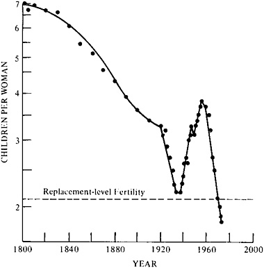
FIGURE 11–1 Total estimated fertility rates in the United States from 1800 to 1976. Source: U.S. Department of Commerce, Bureau of the Census, Estimates of the Population of the United States and Components of Change: 1940–1976, Population Estimates and Projections Series P-25, No. 706 (Washington, D.C.: U.S. Government Printing Office, 1977).
illustrates the two paths, which are approximately linear rather than exponential,‡ and the inset shows the corresponding compound growth rates used by the panel for the subperiods from 1975 to 2010.
The rate of economic growth selected by the panel prompted discussion within the committee and among other participants in the study. Most of the economists express reservations about its likelihood, feeling that a 2 percent average rate of growth would not be consistent with the assumption of full employment. Others point to recent trends of declining growth in productivity and suggest that the growing investment in environmental protection and related areas of health and safety, as well as the shift of employment from the manufacturing to the service sector, will continue to reinforce the trend of declining growth in productivity.

FIGURE 11–2 Estimates and projections of the total population of the United States from 1950 to 2010, showing Bureau of the Census alternative projections from 1975. Source: Adapted from U.S. Department of Commerce, Bureau of the Census, Estimates of the Population of the United States and Components of Change: 1940–1976. Population Estimates and Projections Series P-25, No. 706 (Washington, D.C.: U.S. Government Printing Office, 1977).
The Modeling Resource Group used an average annual rate of growth for GNP of 3.2 percent/yr as their base case, but also showed an alternative low value, corresponding to an average of about 2 percent a year, with even greater deceleration.
|
|
D/C Panel |
MRG-Low |
|
1975–1980 |
2.7 |
3.7 |
|
1980–1990 |
2.3 |
2.7 |
|
1990–2000 |
1.8 |
1.2 |
|
2000–2010 |
1.6 |
0.5 |
The Modeling Resource Group generated its high, low, and base-case projections for the growth of GNP by projecting the changes that might be expected in three determinants of potential GNP over the period 1975–2010. Those leading to the lower rate of growth are the following.
-
Work-force participation declining from 0.73 (its average value from 1950 to 1975) to 0.70 in 2010.
-
Unemployment averaging 6 percent.
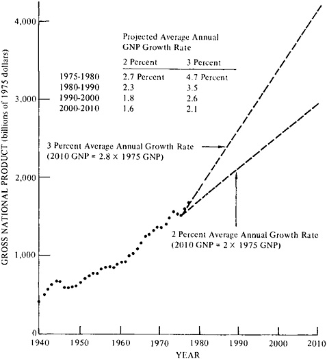
FIGURE 11–3 Past and projected GNP growth in the United States from 1940 to 2010 (billions of 1975 dollars). Source: Adapted from National Research Council, Alternative Energy Demand Futures to 2010, Committee on Nuclear and Alternative Energy Systems, Demand and Conservation Panel (Washington, D.C.: National Academy of Sciences, 1979), p. 60.
-
Growth in productivity shrinking from 1.57 percent per annum in 1975 to zero by 2010.
-
Growth rate of the potential labor force and immigration slowing to 0.2 percent a year after 2010.
Other studies examining the relation of energy consumption and the domestic economy have projected different rates of growth for GNP. The
Energy Policy Project of the Ford Foundation,4 for example, projected three scenarios to the year 2000 (in 1974). In that study, the zero-energy-growth and technical-fix scenarios assumed that GNP would rise at a rate of 3.5 percent/yr from 1975 to 1985, and at a rate of 3.1 percent/yr from 1985 to 2000. The historical-growth scenario assumed that GNP would rise at a rate of 3.6 percent/yr over the first 10-yr period, and at a rate of 3.3 percent/yr from 1985 to 2000. Exxon Corporation5 assumed that GNP would grow over the 4-yr period from 1976 to 1980 at an annual rate of 4.2 percent, and from 1980 to 1990 at an annual rate of 3.4 percent, but warns, “A reasonable range of error in estimating long-term economic growth might be perhaps ±0.5 percent per year.” The Edison Electric Institute6 set out three patterns of economic growth to the year 2010—high, moderate, and low. The high-growth case has GNP rising by 4.2 percent/yr; the moderate case, by 3.5–3.7 percent/yr; and the low case, by 2.3 percent/yr. The institute considers the moderate case to be the most likely. (Table 11–34 gives the annual average GNP growth rates projected by CONAES and other energy studies.)
CONAES did not attempt to select a “best” growth rate, but rather estimated the growth of energy consumption for both 2 percent and 3 percent growth rates in GNP from 1975 to 2010. It is important to recognize that several other estimates are higher than this range and would lead to higher energy consumption for a given set of price assumptions. The scenarios of the Demand and Conservation Panel cannot be regarded as bracketing all the possibilities.
Energy Prices
As recapitulated below, the demand scenarios (presented in chapter 2) assume energy prices held constant (scenario C), doubled (B and B′), or quadrupled (A and A*) by 2010. These are average prices of net delivered energy. The panel assumed specific prices for each source of energy by 2010, displayed in Table 11–2, under the categories of these average prices. The relative prices given in Table 11–2 were intended to reflect approximate parity in dollars per million Btu, with adjustments for the relative cleanliness, convenience, and thermodynamic qualities of fuel. Natural gas is thus priced above distillates, and coal below petroleum. Deregulation of prices was assumed in these projections. Unless otherwise specified, the panel’s overall assumption was that demand would be met at these prices. (Scenarios A* and A, for example, specify a prohibition against the use of natural gas for industrial boilers.)
The assumed prices listed in Table 11–2 for the year 2010 represent those seen by consumers at the final stage of end-use, expressed in 1975 dollars. The relative increase is the same for all consumers, industrial and
residential, and for each end-use. This assumption may overestimate the prices that would be charged for energy consumed in homes and in transportation relative to the prices charged for industrial consumption. It implies that distribution and overhead costs will rise in proportion to primary fuel prices. From 1970 to 1978, in fact, the average costs of primary fuels doubled, but the average prices of delivered energy rose just 30 percent in real dollars.7 Assuming that overhead, distribution, and capital costs remain constant (in constant dollars) while primary fuel costs increase enough to keep average delivered prices the same, a relative shift in demand would occur from industry to households and transportation and from fluid fuels to electricity. The assumed rises in primary fuel prices would have to be more than double the ratios shown in the table. Some trend of this sort is already indicated in the detailed price assumptions. Prices for electricity (with the largest capital and distribution cost) rise least, while prices for natural gas (with the lowest capital and distribution costs) rise most
Other Assumptions
Scenarios A, B, B′, and C assume that the structure of the economy will not change markedly over the next three decades. The energy-price/demand extrapolations employed by the panel are consistent with historical data for fuel-price demand elasticities and cross-elasticities, and with regional comparisons. Details are given in the report of the Demand and Conservation Panel.8
Scenario A*, a simple variant of scenario A, tests the additional moderation in the growth of energy consumption that might result from some changes in the habits and purchases of consumers and from an accelerated shift in the economy from goods to services (for example, from goods produced to be used once and discarded to goods produced to endure with much more repair and maintenance). Again, this scenario might be criticized on the grounds that high labor costs would make repairs uneconomical. On the other hand, it is possible that advances in information technology and microprocessors could greatly increase the productivity of repair services, as well as making possible better quality control and durability in original manufacture (for example, by replacing low-reliability mechanical devices with electronics of higher reliability). Such developments could shift the optimum balance between initial product cost and repair.
TABLE 11–2 Price Assumptions for Scenarios of Energy Demanda
|
|
Oil Prices |
|||||
|
Distillate No. 2b |
Utility Residual |
Gasoline Before Taxes |
||||
|
Dollars per Barrel |
Dollars per Million Btu |
Dollars per Barrel |
Dollars per Million Btu |
Dollars per Barrel |
Dollars per Million Btu |
|
|
1975 actual |
16.37 |
2.81 |
12.40 |
2.02 |
19.08 |
3.64 |
|
2010 scenarios |
|
|
|
|
|
|
|
A, A* |
78.58 |
13.49 |
59.52 |
9.70 |
91.58 |
17.47 |
|
B, B′ |
39.29 |
6.74 |
29.76 |
4.85 |
45.79 |
8.74 |
|
C |
16.37 |
2.81 |
12.40 |
2.02 |
19.08 |
3.64 |
|
Ratios of 2010 prices to 1975 prices |
|
|
|
|
|
|
|
A, A* |
|
4.8 |
|
4.8 |
|
4.8 |
|
B, B′ |
|
2.4 |
|
2.4 |
|
2.4 |
|
C |
|
1.0 |
|
1.0 |
|
1.0 |
|
|
Utility Natural Gas Prices (dollars per million Btu) |
Utility Coalc |
|||||
|
Utilityd |
Residential |
Commercial |
Industriald |
Consumption Weighted Average |
Dollars per Ton |
Dollars per Million Btu |
|
|
1975 actual |
0.75 |
1.70 |
1.41 |
0.99 |
1.29 |
17.68 |
0.81 |
|
2010 scenarios |
|
|
|
|
|
|
|
|
A, A* |
? |
19.63 |
15.89 |
11.38 |
14.84 |
70.52 |
3.24 |
|
B, B′ |
? |
9.82 |
7.94 |
5.69 |
7.42 |
35.26 |
1.62 |
|
C |
? |
4.09 |
3.31 |
2.37 |
3.09 |
17.63 |
0.81 |
|
Ratios of 2010 prices to 1975 prices |
|
|
|
|
|
|
|
|
A, A* |
|
|
|
|
11.5 |
|
4.0 |
|
B, B′ |
|
|
|
|
5.7 |
|
2.0 |
|
C |
|
|
|
|
2.4 |
|
1.0 |
Methodology
The panel investigated the consumption of energy in each of the three principal energy-consuming sectors of the economy—buildings, transportation, and industry—and projected the consumption of energy in these sectors to 2010 under the assumptions of the five scenarios. This sectoral analysis yielded interesting information about energy-efficient technologies and patterns of energy use available for the future, but it did not allow for feedback and other interactions among the sectors. The integrating model was designed to trace the flow of energy through the national economy in 2010, adjusting the energy consumption figures for the three sectors so as to be self-consistent. The energy demand totals for 2010 given here and in chapter 2 were calculated with the aid of the integrating model.
The three sectoral analyses employed different methods, briefly summarized below.
Buildings9 Residential buildings were defined as those occupied by households, and nonresidential buildings as those occupied by the service sectors of the economy. In the residential sector, energy was assumed to be used for space heating, water heating, air conditioning, the preparation and storage of food, lighting, laundry, and the operation of small appliances. In the nonresidential sector, energy was assumed to be used for heating, cooling, and operations such as cleaning and powering elevators.10
An existing engineering-economic simulation model was used to evaluate the effects of rising personal incomes and fuel prices on the cost and use of energy in residential buildings. The model is explained in the report of the Demand and Conservation Panel.11 The panel used this model to simulate the use of four fuels (gas, oil, electricity, and other) for eight functions (space heating, water heating, refrigeration, food freezing, cooking, air conditioning, lighting, and other) in three types of residential buildings (single family, multifamily, and mobile homes). The fuel consumed for each end-use was estimated in response to changes in stocks of occupied housing units and new residential construction, equipment ownership by fuel and end-use, thermal integrity of new and existing housing units, average unit energy requirements for each type of equipment, and aspects of household behavior reflected in patterns of use.
The economic submodels provided the elasticities that determine the responsiveness of households to changes in economic variables (incomes, fuel prices, and equipment prices). The elasticities were calculated for each of the three major household fuels and each of the eight end uses, each fuel price and income elasticity being separated into two elements—the elasticity of equipment ownership and the elasticity of equipment use. The
first gave changes in market shares of equipment ownership in response to changes in fuel prices and incomes; the second gave changes in equipment use with ownership held constant. The submodels also provided equipment-ownership, market-share elasticities with respect to equipment costs. The simulation model was therefore able to estimate consumer responses to changes in operating costs (fuel price times consumption) and changes in capital costs.
The engineering submodels were used to evaluate the variations of purchase prices and energy use with the design of equipment. Detailed submodels were constructed for gas and electric water heaters, refrigerators, and ranges; for the other end-uses, data were combined from various sources to determine relations between energy use and initial cost.
With the simulation model, it was possible to combine the outputs from the various submodels with the initial conditions (from 1970) and the boundary conditions (including policy variables) for the scenario period. The four fuels (i), eight end-uses (k), and three housing types (m) produced 96 fuel-use components (Qi,k,m) for each year (t) of the simulation model. The model also provided annual fuel expenditures, equipment costs, and capital costs for improving the thermal integrity of new and existing structures.
Energy use in the nonresidential subsector was projected by a disaggregated model of the commercial demand for energy12,13 that covered five end-uses (space heating, water heating, cooling, lighting, and other), four fuel types (gas, electricity, oil, and other) and ten commercial subsectors (retail/wholesale, auto repair/garages, office activities, warehouse activities, public administration, education, health care, religious services, hotels/motels, and miscellaneous).
The modeling approach was traditional. The demand for energy, given fuel i, end-use k, and subsector or building type m, was represented simply as
where Q is the energy demand, S the stock of energy-using capital, and U the rate of use.
The stock of equipment was considered fixed over the short term, with only the rate of use changing in response to exogenous factors such as changes in fuel prices. Changes were permitted in the capital stock over the long term in response to rising incomes and the obsolescence of the existing stock.
The energy used in the commercial sector was estimated on the basis of the floor space served. Additions to floor space were calculated by a
desired stock estimate (based on population, per capita income, school-age population, etc.), subtracting additions still standing from previous years.
The use of solar energy was estimated separately for the residential and nonresidential subsectors. The share of the capital market that is likely to be absorbed by solar systems in new buildings was approximated by an ad hoc relationship suggested by the Solar Resource Group of this study. It was assumed that retrofit of solar installations in existing buildings would make a negligible contribution. (This assumption, made before recent federal legislation providing substantial benefits for retrofit of solar installations, may be conservative. See, for example, “Space Heating and Cooling,” in chapter 6.)
Transportation14 Five categories of passenger transportation and four categories of freight transportation were considered in the analysis of this sector.
|
Passenger Transportation |
Freight Transportation |
|
Automobiles |
Truck |
|
Light trucks and vans |
Water |
|
Air travel |
Air |
|
Mass transportation |
Rail |
|
Other |
|
The model employed features of 10 major models constructed over the past 10 years, with a particular view to evaluating the effect on fuel consumption (under the assumptions of the detailed price scenarios shown in Table 11–2) of changes in the efficiency of fuel consumption by vehicles, load factors, prices for fuel, other operating costs, and capital expenditures for transportation. The effects of public policies were assessed by varying the input parameters.
The model assumes that fuel-price ratios (relative to 1975 in 1975 dollars), load factors, and efficiency ratios will increase linearly over the years ahead, but there is considerable uncertainty about the paths they will actually follow. The paths will probably be S-shaped, but since there is also substantial uncertainty about the endpoints (which are more important than the paths), the linear transition actually assumed is not critical. Other assumptions include the following.
-
Automobile travel: Fuel economies of new cars will increase to a plateau by 2000; the average fuel economy of the total fleet will lag behind new-car improvements by 10 years. Gasoline taxes per vehicle-mile (in 1975 dollars) will remain constant on the assumption (based on historical data) that the cost of building and maintaining highways will depend primarily on the vehicle-miles of use. Expenditures-per capita on autos (in 1975 dollars) will saturate; auto ownership itself is reaching saturation,
-
and the time spent in auto travel by each person (now about 50 min/day) is not likely to increase greatly. Data from the United States and other affluent countries indicate that there is a saturation effect in auto ownership at high income levels. Auto ownership in the United States is approaching one vehicle per licensed driver, although it is believed that a firmer upper limit in auto ownership is one vehicle per person of driving age (about 71 percent of the population in the United States).
-
Light-duty trucks and vans: The assumptions for this mode are essentially similar to those for automobiles, except for a slightly higher gasoline tax per vehicle-mile.
-
Air travel: The percentage of passenger transportation dollars spent on air travel will increase with rising incomes and saturation of expenditures on auto travel. The load factor will increase linearly until 2000 and remain constant thereafter. The energy intensity (Btu per passenger-mile) will decrease linearly until 2000 and remain constant thereafter.
-
Mass transportation15 and other passenger modes: All nonfuel operating costs (in 1975 dollars) will remain constant to 2010. For mass transportation, load factors rise in each scenario except B′, as shown below.
|
Average load factors in 2010 by scenario for mass transportation |
|
|
(1975) |
(17.9 passengers per vehicle) |
|
A*, A |
31.0 passengers per vehicle |
|
B |
27.0 passengers per vehicle |
|
C |
22.0 passengers per vehicle |
|
B′ |
17.9 passengers per vehicle |
-
The energy intensity of the vehicles used remains unchanged over the period.
-
All freight modes: The growth in all modes of freight transport per capita will be proportional to the growth in real GNP per capita. Where load factors and efficiencies change, they change linearly during the 1975–2010 period.
Industry16 The analysis of energy consumption in the industrial sector concentrated on 14 industries that account for 80 percent of the energy consumed by industry: 9 energy-consuming industries (agriculture, aluminum, cement, chemicals, construction, food, glass, iron and steel, and paper) and 5 energy-producing industries (oil and gas extraction, oil and gas refining, coal mining, synthetic fuels, and electrical generation). The energy these industries are likely to require in the future was estimated by multiplying the projected level of production for each industry in 2010 by its expected energy intensity. The projected growth
rates are displayed in Table 11–3. The data available to the panel were inadequate for determination of the energy-price/consumption elasticities within individual industries. The panel identified the technologies available for increasing the efficiency of energy use within each of the 14 industries, and estimated the extent to which these might be applied under the assumptions of each scenario. The technological possibilities are indicated qualitatively in Table 11–4.
In projecting the mix of old and new industrial plants for 2010, the panel assumed the prevailing retirement rate: 2 percent/yr for plants in operation in 1975. A third of today’s facilities would thus still be in use in 2010. This assumption may be conservative for the higher-price scenarios, as the energy cost of old equipment might accelerate replacement. In these scenarios, capital not needed for energy supply would be available for accelerated replacement of energy-consuming equipment.
The panel studied the patterns of energy use by the industries named and employed a few additional assumptions to derive preliminary estimates of the fuel mix for industry in 2010. The use of natural gas, for example, was assumed to be increasingly restricted under the assumptions of scenarios A, B, and B′ as a result of higher prices and policies governing scarcer fuels. In these scenarios, the use of natural gas was limited to special applications that justify the use of this high-quality fuel at higher prices (or under the terms of restrictive policies that might be imposed on its use). Since the price of coal is competitive with that of other fuels in the higher-price scenarios, it was assumed that most industrial generation of steam would be fired by coal in scenarios A, B, and B′, and that many existing processes fueled by oil and natural gas would be converted to coal by 2010. Scenario C assumes no restrictions on the availability of natural gas for industrial use.
On the advice of the Supply and Delivery Panel, the Demand and Conservation Panel assumed that solar energy would be economical for some low-temperature industrial applications if the prices of other sources rose appreciably. The panel assumed that the direct use of solar energy would replace that of natural gas to produce low-pressure steam and hot water for agriculture, food processing, and miscellaneous manufacturing processes, accounting for 0.2 quadrillion Btu (quad) of industrial energy consumption in scenario C, for example, and 1.8 quads in scenario A.
Integrating model17 Since the three sectoral analyses were carried out independently, the panel sought some means to array and correct their results in a model of the economy for 2010. The model used national economic data from the U.S. Department of Commerce18 for the year 1967 (the most recent at the time the panel conducted the analysis). Corrections were made for data from the sectoral analyses (using 1975 as
TABLE 11–3 Projection of Industrial Growth Rates from 1975 to 2010
|
Industry |
Growth Rate of Production 1960–1972 (percent per year) |
Ratio of Production Growth Rate to GNP Growth Ratea |
Initial Future Growth Rate Approximationb (percent per year) |
Modified Growth Rates for Final Projections (percent per year) |
Reasonsc for Modification |
||||
|
For 2 percent per year GNP Growth |
For 3 Percent per year GNP Growth |
||||||||
|
A |
B |
B |
C |
||||||
|
Agriculture |
1.6 |
0.39 |
0.8 |
1.2 |
1.7 |
1.7 |
1.7 |
1.7 |
1,2,8 |
|
Aluminum |
6.9 |
1.68 |
3.4 |
5.0 |
3.2 |
3.6 |
5.4 |
4.0 |
3,4 |
|
Cement |
3.6 |
0.88 |
1.8 |
2.6 |
1.8 |
1.8 |
2.6 |
1.8 |
|
|
Chemicals |
8.4 |
2.05 |
4.1 |
6.1 |
3.6 |
3.8 |
4.8 |
4.1 |
3,4,5 |
|
Constructiond |
3.8 |
0.93 |
1.8 |
2.8 |
0.7 |
0.7 |
1.0 |
0.7 |
1,3,6 |
|
Food |
3.3 |
0.80 |
1.6 |
2.4 |
2.2 |
2.2 |
3.2 |
2.2 |
1,8 |
|
Glass |
4.3 |
1.05 |
2.1 |
3.1 |
2.1 |
2.1 |
3.1 |
2.1 |
|
|
Iron and steel |
3.6 |
0.88 |
1.8 |
2.6 |
1.7 |
1.7 |
2.7 |
1.7 |
6,7 |
|
Paper |
5.4 |
1.32 |
2.6 |
3.9 |
1.9 |
1.9 |
2.9 |
1.9 |
5,6,7 |
|
Other manufacturing and mining activities |
4.8 |
1.17 |
2.3 |
3.5 |
2.2 |
2.2 |
3.2 |
2.2 |
6,7 |
|
aThe average growth rate in GNP (constant dollars) was 4.1 percent per year during the 1960–1972 period. bBased on the 1960–1972 ratio of production growth to GNP growth. cThe reasons are as follows: (1) Growth rate for this industry is relatively independent of the GNP growth rate. (2) Exports will cause a slight increase in the prevailing growth rate. (3) Product is energy intensive. High energy prices will lower the otherwise expected growth in demand. (4) Unique properties of products from this industry will tend to increase demand growth. (5) Market saturation will dampen present growth rates. (6) New technological developments will decrease the otherwise expected growth in demand. (7) Competing products will lower the growth rate of production in the United States. (8) Adjusted for assumed lower population growth rate. dAsphalt paving claims about half the energy used by the construction industry. Source: Adapted from National Research Council, Alternative Energy Demand Futures to 2010, Committee on Nuclear and Alternative Energy Systems, Demand and Conservation Panel (Washington, D.C.: National Academy of Sciences, 1979), p. 100. |
|||||||||
TABLE 11–4 Potential for Industrial Energy Conservation for 2010
|
|
Agriculture |
Aluminum |
Cement |
Chemicals |
Constructiona |
Food |
Glass |
Iron and Steel |
Paper |
Other User Industries |
|
Conservation Effect on Consuming Industriesb |
||||||||||
|
Basic “housekeeping” |
|
— |
— |
— |
|
— |
— |
— |
— |
— |
|
More recycling |
|
— |
|
|
— |
|
— |
|
— |
|
|
Environmental controls |
+ |
|
+ |
+ |
|
+ |
|
+ |
+ |
+ |
|
Conversion of gasoline engines to diesel |
— |
|
|
|
|
|
|
|
|
— |
|
Increased yield of product |
+ |
|
|
|
|
|
|
+ |
+ |
+ |
|
Changing product preference |
+ |
|
|
+ |
|
|
|
+ |
+ |
+ |
|
New basic process |
|
— |
— |
— |
|
— |
|
— |
— |
|
|
More waste heat recovery |
|
— |
— |
— |
|
— |
— |
— |
— |
— |
|
Cogeneration |
|
— |
— |
— |
|
— |
|
— |
— |
|
|
Substitute products |
|
|
|
|
— |
— |
|
|
|
|
|
Feedstock demand |
|
|
|
+ |
|
|
|
|
+ |
|
|
Lower-quality raw materials |
|
+ |
|
+ |
|
|
|
+ |
|
|
|
Conversion to electricity |
+ |
+ |
|
|
|
+ |
|
+ |
+ |
+ |
|
Estimated Net Reduction in Energy Intensity by Energy-Consuming Industriesc |
||||||||||
|
Scenario A |
15 |
45 |
40 |
26d |
42 |
34 |
31 |
28 |
36 |
43 |
|
Scenario B |
15 |
37 |
37 |
22d |
35 |
24 |
24 |
24 |
29 |
25 |
|
Scenario B′ |
15 |
37 |
37 |
22d |
35 |
24 |
24 |
24 |
29 |
25 |
|
Scenario C |
5 |
21 |
25 |
16d |
27 |
14 |
18 |
17 |
24 |
15 |
|
aAsphalt only. bA minus indicates reduction in energy intensity; a plus, increased energy intensity. cPercent reduction or increase in energy use per unit of production. dDoes not include chemical feedstocks. Source: Adapted from National Research Council, Alternative Energy Demand Futures to 2010, Committee on Nuclear and Alternative Energy Systems, Demand and Conservation Panel (Washington, D.C.: National Academy of Sciences, 1979), p. 104. |
||||||||||
TABLE 11–5 40 Sectors of the Integrating Model
|
Extraction, Processing, Conversion of Energy Coal mining Crude petroleum, natural gas Shale oil Coal gasification Coal liquefaction Refined petroleum products Natural gas utilities Coal combined-cycle electricity Fossil fuel electric utilities Light water reactors High-temperature gas-cooled reactors Renewable energy utilities |
Production of Goods and Services Agriculture Mining Construction Food Paper Chemicals Glass products Stone and clay products Iron and steel Nonferrous metals Intermediate goods Rail transport Bus transport Truck transport Water transport Air transport Wholesale and retail trades Other services Motor vehicles and equipment Consumer goods |
|
Energy Services, End-Uses Ore-reduction feedstocks Chemical feedstocks Motive power Process heat Water heat Space heat Air conditioning Miscellaneous uses of electricity |
the base year). The Department of Commerce data were supplemented by specific data on new energy technologies and processes to highlight the end-uses of energy and to express consumption of energy in physical, rather than monetary units, as the price of energy varies with the type of purchaser. A 40-sector model was constructed to characterize the economy. Twelve sectors represent the extraction, processing, and conversion of energy resources, 8 represent energy services or end-uses of energy, and the remaining 20 represent the sectors that produce nonenergy goods and services (see Table 11–5).
The interrelation between these sectors make up a 40×40 matrix of input-output coefficients. A typical element A represents the input required from sector i to produce one unit of output from sector j. The matrix manifests the state of technology by indicating the energy intensity (energy needed per unit of output) for the services and products of each sector. The results of the sectoral analyses were used to define the energy intensities and technologies (described below).
The model presents a simplified picture of energy flow through the economy. By tracing this flow through the sectors, the panel was able to derive self-consistent energy consumption figures for the scenarios.
TABLE 11–6 Demand for Energy Projected by Scenario A* for 2010 (quads)a
|
Energy Form |
Industryb |
Buildingsb |
Transportationb |
Total Demandb |
Conversion Lossc |
Primary Energy Input |
Efficiency (percent) |
|
Coal |
9.4 |
0.6 |
0.1 |
10.1 |
— |
10.1 |
100 |
|
Oil |
8.0 |
1.5 |
10.0 |
19.5 |
2.7 |
22.2 |
88 |
|
Gas |
5.8 |
1.6 |
0.1 |
7.5 |
0.5 |
8.0 |
94 |
|
Purchased electricityd |
2.4 |
2.7 |
— |
5.1 |
12.6 |
17.7 |
29 |
|
TOTAL |
25.6 |
6.4 |
10.2 |
42.2 |
15.8 |
58.0 |
73 |
|
aResults are shown to three significant figures to allow display of the small quantities under Transportation. bDemand for energy at point of consumption. cConversion losses include those incurred in extraction, refining, production, transmission, and distribution. dIncludes all energy sources projected for electricity generation—coal, oil, gas, hydroelectric, nuclear, geothermal, and solar. |
|||||||
The panel found it necessary to adopt some accounting conventions for this model. Total primary energy is defined as the total Btu content of the fossil fuels extracted plus the Btu equivalent of energy from hydroelectric, nuclear, solar, and geothermal sources (computed as the heat content of the coal it would take to generate the equivalent amount of electricity). Fossil fuels flow to the energy-producing sectors (for synthetic fuels and generation of electricity) and to the energy-consuming sectors. Tables 11–6 to 11–10 set out the inputs of energy to the energy-consuming sectors and the energy likely to be consumed in producing and distributing these inputs, and Table 11–11 gives figures for 1975. Adding these losses to the inputs flowing into the energy-consuming sectors yields the total primary energy input to the economy.
Each element in the 40×40 matrix (A) may change over the next three decades as production technologies change. Specifying all these possible changes would be a laborious task. The most significant changes (for projecting possible paths of reducing energy consumption through conservation techniques) will occur in those aspects of production technologies that have the greatest effect on demand for energy. To identify these aspects, “energy input fractions” (gi,j below)—each the fraction of the total energy intensity of a product from sector j (∈j) that is
TABLE 11–7 Demand for Energy Projected by Scenario A for 2010 (quads)a
|
Energy Form |
Industryb |
Buildingsb |
Transportationb |
Total Demandb |
Conversion Lossc |
Primary Energy Input |
Efficiency (percent) |
|
Coal |
10.7 |
— |
0.1 |
10.8 |
|
10.8 |
100 |
|
Oil |
8.7 |
2.2 |
14.0 |
24.9 |
3.2 |
28.1 |
89 |
|
Gas |
6.2 |
2.5 |
0.1 |
8.8 |
0.5 |
9.3 |
95 |
|
Purchased electricityd |
2.6 |
4.8 |
— |
7.4 |
18.0 |
25.4 |
30 |
|
TOTAL |
28.2 |
9.5 |
14.2 |
51.9 |
21.7 |
73.6 |
70 |
|
aResults are shown to three significant figures to allow display of the small quantities under Transportation. bDemand for energy at point of consumption. cConversion losses include those incurred in extraction, refining, production. transmission, and distribution. dIncludes all energy sources projected for electricity generation—coal. oil, gas. hydroelectric, nuclear, geothermal, and solar. |
|||||||
TABLE 11–8 Demand for Energy Projected by Scenario B for 2010 (quads)a
|
Energy Form |
Industryb |
Buildingsb |
Transportationb |
Total Demandb |
Conversion Lossc |
Primary Energy Input |
Efficiency (percent) |
|
Coal |
12.6 |
— |
0.1 |
12.7 |
— |
12.7 |
100 |
|
Oil |
10.0 |
2.9 |
19.4 |
32.3 |
5.8 |
38.1 |
85 |
|
Gas |
6.9 |
3.4 |
0.1 |
10.4 |
0.6 |
11.0 |
94 |
|
Purchased elec-tricityd |
3.1 |
6.3 |
— |
9.4 |
22.7 |
32.1 |
29 |
|
TOTAL |
32.6 |
12.6 |
19.6 |
64.8 |
29.1 |
93.9 |
69 |
|
aResults are shown to three significant figures to allow display of the small quantities under Transportation. bDemand for energy at point of consumption. cConversion losses include those incurred in extraction, refining, production, transmission, and distribution. dIncludes all energy sources projected for electricity generation—coal, oil, gas, hydroelectric, nuclear, geothermal, and solar. |
|||||||
TABLE 11–9 Demand for Energy Projected by Scenario B′ for 2010 (quads)a
|
Energy Form |
Industryb |
Buildingsb |
Transportationb |
Total Demandb |
Conversion Lossc |
Primary Energy Input |
Efficiency (percent) |
|
Coal |
17.5 |
— |
0.2 |
17.7 |
— |
17.7 |
100 |
|
Oil |
14.2 |
3.7 |
26.9 |
44.8 |
11.8 |
56.6 |
79 |
|
Gas |
9.6 |
4.6 |
0.2 |
14.4 |
1.4 |
15.8 |
91 |
|
Purchased electricityd |
4.4 |
8.6 |
0.1 |
13.1 |
30.4 |
43.5 |
30 |
|
TOTAL |
45.7 |
16.9 |
27.4 |
90.0 |
43.6 |
133.6 |
67 |
|
aResults are shown to three significant figures to allow display of the small quantities under Transportation. bDemand for energy at point of consumption. cConversion losses include those incurred in extraction, refining, production, transmission, and distribution. dIncludes all energy sources projected for electricity generation—coal, oil, gas, hydroelectric, nuclear, geothermal, and solar. |
|||||||
TABLE 11–10 Demand for Energy Projected by Scenario C for 2010 (quads)a
|
Energy Form |
Industryb |
Buildingsb |
Transportationb |
Total Demandb |
Conversion Lossc |
Primary Energy Input |
Efficiency (percent) |
|
Coal |
9.6 |
— |
0.1 |
9.7 |
— |
9.7 |
100 |
|
Oil |
9.7 |
4.0 |
25.9 |
39.6 |
9.7 |
49.3 |
81 |
|
Gas |
13.9 |
7.0 |
0.1 |
21.0 |
4.8 |
25.8 |
81 |
|
Purchased electricityd |
5.8 |
9.3 |
0.1 |
15.2 |
34.8 |
50.0 |
30 |
|
TOTAL |
39.0 |
20.3 |
26.2 |
85.5 |
49.3 |
134.8 |
64 |
|
aResults are shown to three significant figures to allow display of the small quantities under Transportation. bDemand for energy at point of consumption. cConversion losses include those incurred in extraction, refining, production, transmission, and distribution. dIncludes all energy sources projected for electricity generation—coal, oil, gas, hydroelectric, nuclear, geothermal, and solar. |
|||||||
TABLE 11–11 Demand for Energy in 1975 (quads)a
|
Energy Form |
Industryb |
Buildingsb |
Transportationb |
Total Demandb |
Conversion Lossc |
Primary Energy Input |
Efficiency (percent) |
|
Coal |
3.8 |
0.2 |
— |
4.0 |
— |
4.0 |
100 |
|
Oil |
5.3 |
5.4 |
16.7 |
27.4 |
2.5 |
29.9 |
92 |
|
Gas |
8.6 |
7.6 |
0.6 |
16.8 |
— |
16.8 |
100 |
|
Purchased electricityd |
2.3 |
3.6 |
— |
5.9 |
14.2 |
20.1 |
29 |
|
TOTAL |
20.0 |
16.8 |
17.3 |
54.1 |
16.7 |
70.8 |
76 |
|
aResults are shown to three significant figures to allow display of the small quantities under Transportation. bDemand for energy at point of consumption. cConversion losses include those incurred in extraction, refining, production, transmission, and distribution. dIncludes all energy sources projected for electricity generation—coal, oil, gas, hydroelectric, nuclear, geothermal, and solar. |
|||||||
embodied in the input from sector i (∈j)—were calculated for the base year by the equation
and ordered by rank.
Computing the energy input fractions brought several aspects of energy consumption into sharper focus. In the production of automobiles, for example, calculating the energy input fractions revealed that the energy consumed in assembly accounts for only 10 percent of the total energy cost, while more than a third of the total energy cost can be attributed to the energy used in producing steel. Thus, from the perspective of energy conservation, the size, weight, and material composition of automobiles manufactured in 2010 are more important to the energy consumption than the degree to which assembly is mechanized.
Changes in production techniques were defined by multiplying factors, applied term by term to important elements of the A matrix. Energy can be conserved in two ways in the production of goods and services: by reducing energy inputs, or by replacing these inputs with nonenergy inputs. Industry experts on the panel (and others consulted by the panel) estimated the type and extent of conservation that might be practiced as energy prices rise.
The panel selected the technological changes that seemed most plausible
and assessed their effects under the conditions of various scenarios. (For a detailed description of this model and a complete set of the energy input fractions used to calculate total demand for energy in 2010, see the report of the Demand and Conservation Panel.19
Demand for Electricity
Each of the resource groups of the Demand and Conservation Panel (buildings, industry, and transportation) was asked to estimate the minimum and maximum amounts of purchased electricity required by each of the basic scenarios (A* and B′ being considered variants). The estimation of demand for electricity, as stressed several times in this report, is difficult and controversial.*
The maximum and minimum figures are set out in Table 11–12. The figures for the maximum amount of purchased electricity in the buildings sector proceed from the assumption that almost all space heating in the high-energy scenarios is provided by electricity. The maximum figures for the industrial sector entail the electrification of many processes and no self-generation of electricity. For the maximum figures in the transportation sector, however, the sector is assumed to continue operating primarily on liquid fuels; major advances in the storage of electrical energy (such as high-efficiency batteries) could radically alter this projection.
The penultimate line of Table 11–12 gives the percentage of total primary energy use claimed by electricity in each projection: a range of one quarter to one half. (See also “Electricity” under “Implications of Study Results: Comparisons of Supply and Demand” in this chapter.)
Minimum Energy-Use Scenario (CLOP)20
The Consumption, Location, and Occupational Patterns (CLOP) Resource Group of the Synthesis Panel developed a scenario of energy consumption moderated by shifting attitudes and preferences rather than by rising prices. The group speculated that attitudes emerging in younger generations (for example, thrift in the use of all resources and a preference for environmental quality at the expense of material consumption) might dominate the choices of American society in 2010. Significant changes assumed in the CLOP scenario include major occupational shifts from the employment of individuals in large organizations to self-employment and employment in small groups; increased emphasis on recreational and leisure activities, in forms that consume little material or energy (e.g., cultural activities); and new patterns of settlement that decrease the need
|
* |
See statement 11–4, by R.H.Cannon, Jr., Appendix A. |
TABLE 11–12 Projections of Maximum and Minimum Demand for Purchased Electricity in 2010 (quads)
|
|
Scenario Aa |
Scenario B |
Scenario C |
1975 (actual) |
|||
|
Minimum |
Maximum |
Minimum |
Maximum |
Minimum |
Maximum |
||
|
Buildings |
11 |
22 |
14 |
26 |
21 |
44 |
11 |
|
Industry |
8 |
17 |
9 |
20 |
18 |
23 |
7 |
|
Transportation |
— |
4 |
— |
4 |
— |
4 |
— |
|
TOTAL |
19 |
43 |
23 |
50 |
39 |
71 |
18 |
|
Primary energy |
74 |
94 |
134 |
|
|||
|
Electricity (percent of primary energy) |
26 |
55 |
24 |
53 |
29 |
53 |
28 |
|
Average annual electricity growth (percent)b |
0.2 |
2.5 |
0.7 |
3.0 |
2.2 |
4.0 |
— |
|
aA major shift to electricity for ground transportation is not assumed here. However, if about half of transportation were shifted to electricity by 2010 the additional electrical demand, beginning in 1990, would be approximately 5 GWe/yr. bOver the period 1975–2010. Source: Adapted from National Research Council, Alternative Energy Demand Futures to 2010, Committee on Nuclear and Alternative Energy Systems, Demand and Conservation Panel (Washington, D.C.: National Academy of Sciences, 1979), p. 208. |
|||||||
for energy in transportation. This scenario relies heavily on sophisticated technologies to provide high-quality services and conserve exhaustible resources of energy and materials—solar energy, advanced engine designs, extensive telecommunications systems, and rationalized transportation networks.
Energy consumption in the CLOP scenario totals 53 quads in 2010—a value surprisingly close to that projected by the Demand and Conservation Panel in scenario A* (58 quads), and about half the energy consumed today on a per capita basis. The assumptions of this low-energy projection, however, are distinct. Nuclear power has been phased out, and oil and gas imports have been reduced to zero. The demand for liquid and gaseous fuels is about half that of 1975, and no coal is converted to liquid fuels. The accelerated introduction and expansion of solar technologies in the CLOP scenario result in 10 quads from this source by 2010.
The pattern of energy consumption between 1975 to 2010 was not investigated by the CLOP group.
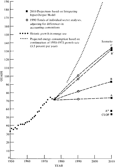
Total Primary Energy Use
Figure 11–4 maps the various paths projected by the Demand and Conservation Panel and shows the endpoints projected by scenario A* and by the CLOP scenario for 2010. These projections were based on the results of the individual sectoral analyses for 1990 and the integrating model for 2010. They indicate how the amount of energy consumed might vary over a wide range—from 53 to 135 quads*—as a result of different prices for energy, rates of growth in GNP, the rate at which available energy-conserving technology is applied, and various public policies. While the projection of lowest growth in the use of energy (A*) assumes some changes in the preferences and life-style choices of energy consumers, these are modest. The projections of the Demand and Conservation Panel depend principally on factors that stimulate (to a greater or lesser degree) the conservation of energy by the application of known technology and practices, rather than depending on fundamental changes in consumer choices or patterns of living and working. This latter pathway to lower energy consumption was investigated qualitatively by the Consumption, Location, and Occupational Patterns Resource Group of the Synthesis Panel, as described in the previous section.
WORK OF THE SUPPLY AND DELIVERY PANEL21
Supply and Delivery Panel was originally expected to generate supply curves, i.e., projections of the amount of each energy form or source that could be produced as a function of time and price. However, the panel concluded that production would be so much influenced by nonprice variables that conventional supply curves would be relatively meaningless. Instead, the panel attempted practical assessments of the conditions of resource recovery and the rate of use of new production technologies, measured against the political and economic forces that influence the decisions of energy resource producers, utilities, and heavy industrial consumers of energy. The practical and judgmental nature of their investigation provides frequent counterpoints to the findings of other panels and resource groups. For example, the Demand and Conservation Panel assumed that under the conditions of their scenarios, sufficient capital would be available for investment in producing the energy
|
* |
See statement 11–5, by R.H.Cannon, Jr., Appendix A. |
resources needed to meet demand in each scenario. The Supply and Delivery Panel replied bluntly that under prevailing conditions, financiers and potential owners would consider investment in new energy supplies to be unacceptably risky, principally because of uncertainties in government policy, regulatory requirements, and delays in acquiring licenses and permits. Thus, for example, the demands projected in scenario B′ could not be met without significant policy changes or greatly increased petroleum imports.
The committee emphasizes that the major point of both panels’ work is that policies enacted to balance energy supply and demand while maintaining satisfactory economic performance must be consistent and sustained. To make the required investments in energy production and end-use capital, consumers and suppliers must be able to read these policies as clear signals encouraging, maintaining, or discouraging various levels of production or end-use. In practice, given policies are likely to be read as different signals by the producers of each energy resource. The Supply and Delivery Panel asked each of its resource groups to estimate the production of its resource or energy form under three sets of conditions and assumptions: business as usual, enhanced supply, and national commitment. The specific conditions assumed for each of these categories varied with the resource. In general, the business-as-usual estimates assumed that existing policies and practices22 carry over into the future with little change. Enhanced-supply estimates assumed that promising new supply technologies are encouraged by policies effected for energy resource production; for example, relaxing environmental standards, or reducing and expediting required regulatory processes. The national-commitment estimates assumed that the policies and regulatory actions of enhanced supply are pursued with urgency. It must be emphasized that policies of national commitment cannot be effected simultaneously for all supply sources. Giving very high priority to the development of one source necessarily implies lower priority and less stimulus to the development of other sources.23
The Supply and Delivery Panel’s resource groups reviewed available estimates of reserves and resources, as well as their producibility, and selected those that matched their consensus judgment. In addition, they considered the availability of the various energy supply technologies during the period to 2010 for each of the three sets of assumed conditions. Table 11–13 displays the estimates of each resource group under the three categories of policy.
The specific assumptions made by each group are set out in Table 11–14. The Supply and Delivery Panel emphasizes that neither table should be read as representing self-consistent sets of possibilities. Many of these estimates presume success with technologies that either have not yet been
tested or have been demonstrated only on small scales. It is possible that some of the prospective technologies on which these estimates are based cannot be successfully developed with any level of commitment. On the other hand, new supplies from unexpected discoveries (of unconventional gas, for example) or from unexpected technical progress in certain technologies (such as solar photovoltaics or coal liquefaction) could outstrip specific estimates.
Maximum-Solar Scenario
To analyze the extent to which solar energy can substitute for other fuels, a “maximum solar” scenario was developed by the Solar Resource Group of the Supply and Delivery Panel.24 It represents an estimate of the maximum feasible application of solar energy between now and 2010, from the point of view of technical, rather than economic, feasibility. The group concluded that increased energy prices, within the range considered by the study, would not be sufficient to stimulate widespread use of solar energy by 2010. Heavy subsidies and government mandates would be needed to encourage installation of solar energy systems in that period to the extent described by the maximum-solar scenario.
This scenario assumes that a national policy decision has been made by 1985 to encourage the use of solar energy in all its applications. The government mandates that solar energy be used to supply heat, air conditioning, and hot water to all new buildings, and to supply industrial process heat where technically feasible. A schedule is set in motion for several solar electric central generating stations, and state and local governments are ordered to adopt as rapidly as possible technologies for converting municipal and agricultural wastes to useful energy. These installations might be financed in part from revenues received from taxing nonrenewable energy sources, a practice that would also help make the solar installations more competitive.
Estimates for the maximum potential application of solar energy are set out in Table 11–15. These numbers represent an effective upper bound on solar energy production. Whether this quantity and mix could be effectively used depends on prevailing conditions. The panel made no attempt to estimate the cost of achieving this projection. More details about this scenario and its context in the study are given in chapter 6.
CONAES Projections of Supply Versus Other Projections
For ready comparison, the estimates of the Supply and Delivery Panel for the year 2000 and the year 2010 are compared to the most recent midrange
TABLE 11–13 Domestic Energy Production for Three Sets of Assumed Conditions (quads per year)a
|
Scenario and Energy Source |
Year |
|||
|
1977 |
1990 |
2000 |
2010 |
|
|
Business as usualb |
|
|
|
|
|
Crude oil |
19.6 |
16.0 |
12.0 |
6.0 |
|
Natural gas |
19.4 |
10.3 |
7.0 |
5.0 |
|
Oil shale |
0 |
0 |
0 |
0 |
|
Synthetic liquidsc |
0 |
(0.3) |
(2.3) |
(6.1) |
|
Synthetic gasc |
0 |
(1.3) |
(3.5) |
(4.1) |
|
Coal |
16.4 |
25.0 |
34.0 |
42.0 |
|
Geothermal |
0 |
0.4 |
0.9 |
2.4 |
|
Solar |
0 |
0 |
0.1 |
0.6 |
|
Nuclear |
2.7 |
10.0 |
12.5 |
15.8 |
|
Hydroelectric |
2.4 |
4.0 |
5.0 |
5.0 |
|
Enhanced supplyb |
|
|
|
|
|
Crude oil |
19.6 |
20.0 |
18.0 |
16.0 |
|
Natural gas |
19.4 |
15.8 |
15.0 |
14.0 |
|
Oil shale |
0 |
0.7 |
1.0 |
1.5 |
|
Synthetic liquidsc |
0 |
(0.4) |
(2–4) |
(8.0) |
|
Synthetic gasc |
0 |
(1.7) |
(3.5) |
(4.8) |
|
Coal |
16.4 |
26.6 |
37.2 |
49.5 |
|
Geothermal |
0 |
0.6 |
1.6 |
4.1 |
|
Solar |
0 |
1.7 |
5.9 |
10.7 |
|
Nuclear |
2.7 |
13.0 |
29.5 |
41.7 |
|
Hydroelectric |
2.4 |
4.1 |
5.0 |
5.0 |
|
National commitmentb |
|
|
|
|
|
Crude oil |
19.6 |
21.0 |
20.0 |
18.0 |
|
Natural gas |
19.4 |
18.0 |
17.0 |
16.0 |
|
Oil shale |
0 |
2.0 |
2.5 |
3.0 |
|
Synthetic liquidsc |
0 |
(0.7) |
(4.7) |
(12.9) |
|
Synthetic gasc |
0 |
(1.7) |
(4.5) |
(7.9) |
|
Coal |
16.4 |
32.5 |
75.0 |
100.0 |
|
Geothermal |
0 |
2.2 |
7.8 |
19.9 |
|
Solar |
0 |
3.3 |
13.1 |
28.8 |
|
Nuclear |
2.7 |
12.0 |
27.5 |
42.5 |
|
Hydroelectric |
2.4 |
4.1 |
5.0 |
5.0 |
|
aExcept for the business-as-usual projections, the entries in this table should not be added to obtain yearly totals; no more than a very few energy sources or technologies could be simultaneously accorded the priorities implied by the enhanced-supply or national-commitment scenarios. bFor specific assumptions guiding selection of estimates under this set of conditions, see Table 11–14. cSynthetic fuels are produced from coal and oil shale and are not added in the totals. Source: Compiled from National Research Council, U.S. Energy Supply Prospects to 2010, Committee on Nuclear and Alternative Energy Systems, Supply and Delivery Panel (Washington, D.C.: National Academy of Sciences, 1979). |
||||
TABLE 11–14 Assumptions Specific to Energy Resource Estimates
|
Energy Source |
Scenarioa |
||
|
Business as Usual |
Enhanced Supply |
National Commitment |
|
|
Coal |
Production limited by difficulties teasing federal land; increasing costs and delays from lack of consistent environmental policies |
Increased demand from enactment of consistent environmental policies |
Rising worker productivity; availability of more capital; streamlined regulatory policies |
|
Oil and gas |
Price controls discourage domestic production; separate permits required for exploration and production in outer continental shelf; delays in leasing; withdrawal of public lands |
Accelerated federal offshore leasing; lifting of controls on wellhead prices; streamlined permit processes; improved exploration and production technologies |
Relaxation of Clean Air standards; streamlined procedures for environmental impact statements; federal loan guarantees for development and application of new technologies; federal return of withdrawn lands; assignment of priority status to materials and labor for oil exploration and recovery |
|
Coal-based synthetics (oil and gas) |
Federal nonrecourse loans for a limited number of new plants: design and construction of such plants takes 6 years (production in seventh year) |
Permits for mining, plant construetion, and operation acted upon within 12 months: design and construction of such plants takes 5 years |
Government agency established to underwrite prices, expedite approval of permits, act to ensure priority assignment of labor, capital, and materials, and so on: design and construction of plants takes 4 years |
projection (Series C) of the Energy Information Administration (EIA)25 in Table 11–16. The EIA projections were made in 1978.
The EIA projections for both oil and gas, assuming enhanced-recovery techniques, are above even the national-commitment scenario of the Supply and Delivery Panel—about 30 percent above in the case of oil, and 20 percent above in the case of gas. The projection of oil and gas production in the year 2000, including enhanced recovery and all synthetics, totals 62.7 quads in the Series C projections of EIA. For 2010, the production of oil and gas, including all synthetics, totals 67.0 quads in the Series C projection. The Supply and Delivery Panel projects oil and gas production of 50.4 quads in 2000 and 58.3 quads in 2010 under the conditions of the national-commitment scenario. The CONAES projections for fluid fuels appear conservative in this context. Nevertheless, additions to domestic oil reserves in 1978 were only 1.3 billion barrels, compared to production of 3.2 billion barrels. To maintain domestic production of oil through the 1980s would require an average annual finding rate of 4.0 billion barrels.26
Several additional points of comparison emerge from inspection of Table 11–16:
-
The EIA projections for coal-derived synthetic liquids agree quite well with those of the enhanced-supply scenario for both 2000 and 2010.
-
The EIA projections for oil shale are near those of the national-commitment scenario, particularly for 2010,
-
If the high- and low-Btu gas projections cast by the EIA are combined, the total corresponds very closely to the national-commitment projections for synthetic gas. Again we see that the CONAES supply projections are on the pessimistic side.
-
The EIA nuclear projections lie midway between the business-as-usual and enhanced-supply projections.
-
The EIA coal projections lie between the enhanced-supply and national-commitment projections of the Supply and Delivery Panel—closer to enhanced supply.
IMPLICATIONS OF STUDY RESULTS: COMPARISONS OF SUPPLY AND DEMAND
Attempts to draw on the understanding and data emerging from one another’s work were important aspects of the work of the several panels and resource groups. In attempting to specify the mix of energy sources appropriate to their scenarios of demand, for example, the Demand and Conservation Panel consulted with members of the Supply and Delivery
TABLE 11–15 Maximum-Solar Scenario
|
Solar Application or Source |
Contribution (quads) |
|
|
1990 |
2010 |
|
|
Space heat, hot water, and nonresidential air conditioning |
0.7 |
4.4 |
|
Municipal wastes |
0.8 |
1.9 |
|
Agricultural residues |
0.9 |
3.5 |
|
Solar and wind electricity |
0.6 |
12.4 |
|
Industrial process heat |
0.4 |
6.6 |
|
TOTAL |
3.4 |
28.8 |
|
Source: Compiled from National Research Council, U.S. Energy Supply Prospects to 2010. Committee on Nuclear and Alternative Energy Systems, Supply and Delivery Panel (Washington, D.C.: National Academy of Sciences, 1979). |
||
Panel. The interaction of supply and demand began with final demand numbers for electricity and for gaseous and liquid fuels. The Supply and Delivery Panel reviewed these demand numbers and rejoined with recommendations modifying the characteristics of demand (asking, for example, “Can some of these demands for liquids be met by electricity?"). The resulting accommodations eventually produced the mix presented in the report of the Demand and Conservation Panel (summarized in Tables 11–6 to 11–10).
The committee staff carried these preliminary attempts further to generate integrated scenarios of supply and demand for the year 2010. These provide numerical examples that illustrate some qualitative conclusions of the study, Although these examples are presented in tables and graphs, they should not be interpreted as predictions, nor can any single scenario be regarded as a preferred path for the next three decades, There was sufficient disagreement among CONAES members about what was socially desirable and politically feasible to preclude the development of any “most likely” or “most desirable” scenario. The numerical values were arrived at judgmentally and should not be regarded as the outcome of a complete chain of inference from a formal model and assumptions, although models were used as a partial guide to judgment
TABLE 11–16 Comparison of Energy-Supply Projections to Midrange Projections of Energy Information Administration (quads)
|
Energy Source |
Supply and Delivery Panel |
Energy Information Administration |
||
|
Business as Usual |
Enhanced Supply |
National Commitment |
||
|
1990 |
|
|
|
|
|
Coal |
25.0 |
26.6 |
32.5 |
31.2 |
|
Oil |
16.0 |
20.0 |
21.0 |
23.1 |
|
Gas |
10.3 |
15.8 |
18.0 |
17.4 |
|
Nuclear |
10.0 |
13.0 |
12.0 |
9.4 |
|
2000 |
|
|
|
|
|
Coal |
34.0 |
37.2 |
75.0 |
46.9 |
|
Oil (1) |
|
|
|
17.8 |
|
Oil (2) |
12.0 |
18.0 |
20.0 |
23.2 |
|
Shale |
0.0 |
1.0 |
2.5 |
1.8 |
|
Synthetic liquids |
2.3 |
2.4 |
4.7 |
2.6 |
|
Gas (1) |
|
|
|
15.8 |
|
Gas (2) |
7.0 |
15.0 |
17.0 |
19.2 |
|
High-Btu gas |
3.5 |
3.5 |
4.5 |
0.4 |
|
Low-Btu gas |
|
|
|
4.1 |
|
Nuclear |
12.5 |
29.5 |
27.5 |
16,9 |
|
2010 |
|
|
|
|
|
Coal |
42.0 |
49.5 |
100.0 |
65.2 |
|
Oil (1) |
|
|
|
13.9 |
|
Oil (2) |
6.0 |
16.0 |
18.0 |
19.6 |
|
Shale |
0.0 |
1.5 |
3.0 |
3.6 |
|
Synthetic liquids |
6.1 |
8.0 |
12,9 |
7.2 |
|
Gas (1) |
|
|
|
11.6 |
|
Gas (2) |
5.0 |
14.0 |
16.0 |
15.2 |
|
High-Btu gas |
4.1 |
4.8 |
7.9 |
1.6 |
|
Low-Btu gas |
|
|
|
6.8 |
|
Nuclear |
15.8 |
41.7 |
42.5 |
29.2 |
|
Sources: National Research Council, U.S. Energy Supply Prospects to 2010, Committee on Nuclear and Alternative Energy Systems, Supply and Delivery Panel (Washington, D.C.: National Academy of Sciences, 1979); and U.S. Department of Energy, Energy Information Administration, Annual Report to Congress, 1978, vol. 3, Forecasts (Washington, D.C.: U.S. Department of Energy, 1979). |
||||
THE STUDY SCENARIOS27
To compare the projections of energy demand from the Demand and Conservation Panel with the projections of energy supplies from the Supply and Delivery Panel, a variant of the demand projections was prepared by scaling demand scenarios A*, A, and C for 3 percent annual average growth of GNP, based on the comparison of demand scenarios B
and B′. The study scenarios are distinguished by roman numerals (low to high consumption of energy) and subscripts (2 or 3 percent growth of GNP). Study scenario I2 corresponds to demand scenario A*, for example, and study scenarios III2 and III3 correspond to demand scenarios B and B′.
To prepare the projections for comparison with those of the Supply and Delivery Panel, the following changes were made.
-
The demand projections include an 8 percent loss in the distribution of oil. These losses were added to the total figure for demand at the point of consumption to yield total primary demand for oil.
-
The demand projections include a minimum and a maximum figure for electricity purchased by industry, corresponding to maximum and minimum figures (respectively) for the cogeneration and self-generation of electricity by industry (Table 11–12). The study scenarios assume industrial demand for electricity approximately at the midpoint of these two projections. The corresponding decrease in primary fuel use shows up in the demand-supply comparisons principally as lower demand for coal by industry.
-
The figures for substitution of solar energy for direct use of fuels and electricity in buildings and industry, and the figures for the use of “other” sources in industry (such as sawdust burned in paper mills), were taken from the sectoral analyses of the Demand and Conservation Panel and were added to the projections.
-
Following the suggestion of the Industry Resource Group of the Demand and Conservation Panel that gas and oil are readily interchangeable in about 50 percent of industrial applications, the study scenarios assume that industry will use natural gas to fill somewhat less than 50 percent of its projected demand for oil (the percentage varies with scenario, depending on the relative prices and availability of these fuels).
The basic principles guiding the comparison of demand and supply scenarios were (1) to assume with the Demand and Conservation Panel that energy-efficient technology would be adopted over the period 1975– 2010 to the extent economically justified under the assumed schedules of price, and (2) to fill scenarios of demand from the Supply and Delivery Panel scenarios that best matched the assumed conditions. For example, the scenarios of low demand were generally compared to business-as-usual scenarios of supply, unless the demand for a particular energy form was greater than business-as-usual supply projections could meet.
Although the assignment of production levels from the Supply and Delivery Panel’s scenarios to the Demand and Conservation Panel’s scenarios of demand was an exercise of judgment, there is actually less
room for maneuver and arbitrariness than might be supposed. Coal and nuclear fuels can be substituted for one another in the generation of electricity, for example, but because of competitive demands for coal to produce synthetic fluids, the growth of coal consumption must be very large if some growth in nuclear power is not also maintained (except in the cases of lowest assumed growth in demand). A more significant finding of this exercise is that the demand for fluid fuels cannot be met by business-asusual supply projections, even in the cases of the lowest projected growth in demand, without rising imports. The scenarios of high demand require energy production levels from the Supply and Delivery Panel’s national-commitment scenarios. The complete set of scenarios is displayed in Tables 11–17 to 11–24.
It is convenient for discussion to classify these scenarios in four groups—“low energy consumption” (CLOP, I2, I3, II2), “low-medium” (II3 and IV2), “high-medium” (III3 and IV2), and “high” (IV3). Their range in 2010 and the courses of their development are illustrated in Figures 11–5 and 11–6. To indicate their range, this section compares for discussion study scenarios I2, II2, III2, and III3, and IV3.
Nuclear Power
The demand for nuclear energy was met by business-as-usual levels of installation and operation in scenarios I2 and II2, by enhanced-supply conditions in scenarios III2 and III3, and by national-commitment conditions in scenario IV3. The Supply and Delivery Panel has expressed the opinion that the nuclear industry possesses the physical and organizational capacity to deploy considerably more nuclear power than is required even for scenario IV3. In the scenarios developed by the Supply and Delivery Panel, the achievable growth rate of installed nuclear capacity increases rapidly after 1990 (as indicated in Table 11–13).
The Demand and Conservation Panel’s projections of demand for electricity, on the other hand, show much more rapid growth in demand for electricity before 1990 than after (as indicated in chapter 2). Thus, the study scenarios do not require nearly so much installed nuclear capacity in 2010 as the Supply and Delivery Panel states is possible. In low-consumption scenarios I2 and II2, the use of nuclear power actually declines after 1990, following the general trend of demand for electricity. In medium-growth scenario III2, the use of nuclear power remains fairly constant after 1990, again following the trend of demand for electricity. In high-medium and high-consumption scenarios III3 and IV3, nuclear power continues to grow after 1990, but at a rate below the maximum considered possible by the Supply and Delivery Panel.
TABLE 11–17 Fuel Mix Projected by Study Scenario I2 (quads per year)
|
Energy Source |
1975 |
1990 |
2010 |
Required Supply Conditionsa |
|
Oil |
|
|
|
|
|
Domestic |
20 |
18 |
11 |
BAU, ES |
|
Imported |
13 |
5 |
12 |
— |
|
Shale |
0 |
0 |
0 |
BAU |
|
Gas |
|
|
|
|
|
Domestic |
19 |
13 |
8 |
BAU, ES |
|
Imported |
1 |
0 |
0 |
— |
|
Coal |
|
|
|
|
|
Combustion |
13 |
20 |
15 |
BAU |
|
Conversion to synthetic liquid |
0 |
0 |
0 |
BAU |
|
Conversion to synthetic gas |
0 |
0 |
0 |
BAU |
|
Nuclear |
2 |
8 |
6 |
BAU |
|
Solar |
0 |
1 |
6 |
ES |
|
Other (hydro, geothermal, etc.) |
3 |
5 |
6 |
BAU |
|
TOTAL |
71 |
70 |
64 |
|
|
TOTAL, liquid fuelsb |
33 |
23 |
23 |
|
|
TOTAL, gaseous fuelsb |
20 |
13 |
8 |
|
|
TOTAL, electricityc |
20 |
25 |
17 |
|
|
aThe Supply and Delivery Panel based its estimates of energy source availability on sets of assumptions about regulatory policies and public attitudes, which were judged more likely to determine availability than cost or price. These assumptions are as follows: Business as usual (BAU)—existing attitudes, policies, and practices are extended into the future with little change; integrated, effective energy supply policies are not established and implemented. Enhanced supply (ES)—a well-balanced, comprehensive set of energy supply policies is enacted and aggressively pursued; decision making and regulatory actions are timely and coordinated; and promising new technologies are appropriately supported. National commitment (NC)—the same comprehensive set of energy policies is pursued as in the enhancedsupply case, but more aggressively in specific areas; adequate energy supplies are given the highest priority in allocating national resources; and calculated risks are taken in deploying promising new energy technologies before they are economically practicable. bIncludes losses in production and distribution, but not conversion for synthetic fuels derived from coal. cIncludes conversion losses. |
||||
Electricity
As noted earlier in this chapter, there is considerable uncertainty today in the projection of demand for electricity. If the demand for electricity in 2010 were to fall near the upper end of the range projected by the Demand and Conservation Panel, significantly larger installed nuclear capacity
TABLE 11–18 Fuel Mix Projected by Study Scenario I3 (quads per year)
|
Energy Source |
1975 |
1990 |
2010 |
Required Supply Conditionsa |
|
Oil |
|
|
|
|
|
Domestic |
20 |
21 |
18 |
NC |
|
Imported |
13 |
8 |
13 |
— |
|
Shale |
0 |
0 |
0 |
BAU |
|
Gas |
|
|
|
|
|
Domestic |
19 |
14 |
11 |
BAU, ES |
|
Imported |
1 |
1 |
0 |
— |
|
Coal |
|
|
|
|
|
Combustion |
13 |
27 |
25 |
BAU |
|
Conversion to synthetic liquid |
0 |
0 |
0 |
BAU |
|
Conversion to synthetic gas |
0 |
0 |
0 |
BAU |
|
Nuclear |
2 |
8 |
6 |
BAU |
|
Solar |
0 |
1 |
6 |
ES |
|
Other (hydro, geothermal, etc.) |
3 |
5 |
6 |
BAU |
|
TOTAL |
71 |
85 |
85 |
|
|
TOTAL, liquid fuelsb |
33 |
29 |
31 |
|
|
TOTAL, gaseous fuelsb |
20 |
15 |
11 |
|
|
TOTAL, electricityc |
20 |
31 |
23 |
|
|
aThe Supply and Delivery Panel based its estimates of energy source availability on sets of assumptions about regulatory policies and public attitudes, which were judged more likely to determine availability than cost or price. These assumptions are as follows: Business as usual (BAU)—existing attitudes, policies, and practices are extended into the future with little change; integrated, effective energy supply policies are not established and implemented. Enhanced supply (ES)—a well-balanced, comprehensive set of energy supply policies is enacted and aggressively pursued; decision making and regulatory actions are timely and coordinated; and promising new technologies are appropriately supported. National commitment (NC)—the same comprehensive set of energy policies is pursued as in the enhancedsupply case, but more aggressively in specific areas; adequate energy supplies are given the highest priority in allocating national resources; and calculated risks are taken in deploying promising new energy technologies before they are economically practicable. bIncludes losses in production and distribution, but not conversion for synthetic fuels derived from coal. cIncludes conversion losses. |
||||
would be required, and nuclear growth rates closer to those projected by the Supply and Delivery Panel would be shown by the scenarios. For example, the demand for electricity in scenario IV3 requires 71 quads of primary energy input, of which 30 quads (corresponding to 600 gigawatts (electric) (GWe) of installed capacity) is provided by nuclear power—only slightly less than the enhanced-supply scenario value of 35 quads.
TABLE 11–19 Fuel Mix Projected by Study Scenario II2 (quads per year)
|
Energy Source |
1975 |
1990 |
2010 |
Required Supply Conditionsa |
|
Oil |
|
|
|
|
|
Domestic |
20 |
18 |
11 |
BAU, ES |
|
Imported |
13 |
5 |
10 |
— |
|
Shale |
0 |
0 |
1 |
BAU, ES |
|
Gas |
|
|
|
|
|
Domestic |
19 |
13 |
10 |
BAU, ES |
|
Imported |
1 |
0 |
3 |
— |
|
Coal |
|
|
|
|
|
Combustion |
13 |
25 |
22 |
BAU |
|
Conversion to synthetic liquid |
0 |
0 |
6 |
BAU |
|
Conversion to synthetic gas |
0 |
0 |
0 |
BAU |
|
Nuclear |
2 |
8 |
7 |
BAU |
|
Solar |
0 |
1 |
4 |
ES |
|
Other (hydro, geothermal, etc.) |
3 |
6 |
9 |
ES |
|
TOTAL |
71 |
76 |
83 |
|
|
TOTAL, liquid fuelsb |
33 |
23 |
26 |
|
|
TOTAL, gaseous fuelsb |
20 |
13 |
13 |
|
|
TOTAL, electricityc |
20 |
31 |
29 |
|
|
aThe Supply and Delivery Panel based its estimates of energy source availability on sets of assumptions about regulatory policies and public attitudes, which were judged more likely to determine availability than cost or price. These assumptions are as follows: Business as usual (BAU)—existing attitudes, policies, and practices are extended into the future with little change; integrated, effective energy supply policies are not established and implemented. Enhanced supply (ES)—a well-balanced, comprehensive set of energy supply policies is enacted and aggressively pursued; decision making and regulatory actions are timely and coordinated; and promising new technologies are appropriately supported, National commitment (NC)—the same comprehensive set of energy policies is pursued as in the enhancedsupply case, but more aggressively in specific areas; adequate energy supplies are given the highest priority in allocating national resources; and calculated risks are taken in deploying promising new energy technologies before they are economically practicable. bIncludes losses in production and distribution, but not conversion for synthetic fuels derived from coal. cIncludes conversion losses. |
||||
Scenarios of higher electrical demand, calling for even more nuclear capacity, could be envisaged. The Edison Electric Institute, for example, projects a demand for electrical generation of almost 80 quads in the year 2000.28 Under these assumed conditions, the national-commitment level of nuclear capacity would be required.
An illustrative example of higher electricity demand can be envisioned
TABLE 11–20 Fuel Mix Projected by Study Scenario II3 (quads per year)
|
Energy Source |
1975 |
1990 |
2010 |
Required Supply Conditionsa |
|
Oil |
|
|
|
|
|
Domestic |
20 |
21 |
18 |
NC |
|
Imported |
13 |
7 |
11 |
— |
|
Shale |
0 |
0 |
2 |
ES |
|
Gas |
|
|
|
|
|
Domestic |
19 |
15 |
14 |
ES |
|
Imported |
1 |
0 |
2 |
— |
|
Coal |
|
|
|
|
|
Combustion |
13 |
31 |
35 |
BAU |
|
Conversion to synthetic liquid |
0 |
0 |
9 |
BAU, ES |
|
Conversion to synthetic gas |
0 |
0 |
3 |
BAU |
|
Nuclear |
2 |
8 |
8 |
BAU |
|
Solar |
0 |
1 |
4 |
ES |
|
Other (hydro, geothermal, etc.) |
3 |
6 |
9 |
ES |
|
TOTAL |
71 |
89 |
115 |
|
|
TOTAL, liquid fuelsb |
33 |
28 |
37 |
|
|
TOTAL, gaseous fuelsb |
20 |
15 |
18 |
|
|
TOTAL, electricityc |
20 |
36 |
39 |
|
|
aThe Supply and Delivery Panel based its estimates of energy source availability on sets of assumptions about regulatory policies and public attitudes, which were judged more likely to determine availability than cost or price. These assumptions are as follows: Business as usual (BAU)—existing attitudes, policies, and practices are extended into the future with little change; integrated, effective energy supply policies are not established and implemented, Enhanced supply (ES)—a well-balanced, comprehensive set of energy supply policies is enacted and aggressively pursued; decision making and regulatory actions are timely and coordinated; and promising new technologies are appropriately supported. National commitment (NC)—the same comprehensive set of energy policies is pursued as in the enhanced-supply case, but more aggressively in specific areas; adequate energy supplies are given the highest priority in allocating national resources; and calculated risks are taken in deploying promising new energy technologies before they are economically practicable. bIncludes losses in production and distribution, but not conversion for synthetic fuels derived from coal. cIncludes conversion losses. |
||||
by varying the assumptions of the study scenarios. Suppose that half the demand for fluid fuels in the buildings sector were replaced by demand for electrical resistance heat. (The projections used for the base cases in this example are study scenarios that assume 3 percent annual average growth of GNP, as shown in Table 11–25, rather than the scenarios of the Demand and Conservation Panel) In scenario I3, the primary demand for liquid
TABLE 11–21 Fuel Mix Projected by Study Scenario III2 (quads per year)
|
Energy Source |
1975 |
1990 |
2010 |
Required Supply Conditionsa |
|
Oil |
|
|
|
|
|
Domestic |
20 |
20 |
16 |
ES |
|
Imported |
13 |
9 |
7 |
— |
|
Shale |
0 |
0 |
1 |
ES |
|
Gas |
|
|
|
|
|
Domestic |
19 |
14 |
14 |
ES |
|
Imported |
1 |
0 |
2 |
— |
|
Coal |
|
|
|
|
|
Combustion |
13 |
24 |
26 |
BAU |
|
Conversion to synthetic liquid |
0 |
1 |
12 |
ES |
|
Conversion to synthetic gas |
0 |
0 |
0 |
BAU |
|
Nuclear |
2 |
11 |
13 |
ES |
|
Solar |
0 |
1 |
3 |
ES |
|
Other (hydro, geothermal, etc.) |
3 |
5 |
8 |
ES |
|
TOTAL |
71 |
85 |
102 |
|
|
TOTAL, liquid fuelsb |
33 |
29 |
32 |
|
|
TOTAL, gaseous fuelsb |
20 |
14 |
16 |
|
|
TOTAL, electricityc |
20 |
33 |
37 |
|
|
aThe Supply and Delivery Panel based its estimates of energy source availability on sets of assumptions about regulatory policies and public attitudes, which were judged more likely to determine availability than cost or price. These assumptions are as follows: Business as usual (BAU)—existing attitudes, policies, and practices are extended into the future with little change; integrated, effective energy supply policies are not established and implemented. Enhanced supply (ES)—a well-balanced, comprehensive set of energy supply policies is enacted and aggressively pursued; decision making and regulatory actions are timely and coordinated; and promising new technologies are appropriately supported. National commitment (NC)—the same comprehensive set of energy policies is pursued as in the enhanced-supply case, but more aggressively in specific areas; adequate energy supplies are given the highest priority in allocating national resources; and calculated risks are taken in deploying promising new energy technologies before they are economically practicable. bIncludes losses in production and distribution, but not conversion for synthetic fuels derived from coal. cIncludes conversion losses. |
||||
and gaseous fuels in buildings totals 10.5 quads. If the efficiency of building heat averages 60 percent (i.e., 40 percent of the heat is lost up the chimney), then the delivered useful heat totals 0.6×10.5 quads, or 6.30 quads. If half this amount were supplied by electrical resistance heat, the requirement would be one half of 6.30 quads, or 3.15 quads of electricity.
TABLE 11–22 Fuel Mix Projected by Study Scenario III3 (quads per year)
|
Energy Source |
1975 |
1990 |
2010 |
Required Supply Conditionsa |
|
Oil |
|
|
|
|
|
Domestic |
20 |
21 |
18 |
NC |
|
Imported |
13 |
16 |
14 |
— |
|
Shale |
0 |
0 |
2 |
ES |
|
Gas |
|
|
|
|
|
Domestic |
19 |
14 |
14 |
ES |
|
Imported |
1 |
1 |
1 |
— |
|
Coal |
|
|
|
|
|
Combustion |
13 |
29 |
34 |
ES, NC |
|
Conversion to synthetic liquid |
0 |
2 |
19 |
NC |
|
Conversion to synthetic gas |
0 |
1 |
7 |
ES |
|
Nuclear |
2 |
11 |
18 |
ES |
|
Solar |
0 |
1 |
3 |
ES |
|
Other (hydro, geothermal, etc.) |
3 |
5 |
10 |
ES |
|
TOTAL |
71 |
101 |
140 |
|
|
TOTAL, liquid fuelsb |
33 |
38 |
47 |
|
|
TOTAL, gaseous fuelsb |
20 |
16 |
20 |
|
|
TOTAL, electricityc |
20 |
38 |
48 |
|
|
aThe Supply and Delivery Panel based its estimates of energy source availability on sets of assumptions about regulatory policies and public attitudes, which were judged more likely to determine availability than cost or price. These assumptions are as follows: Business as usual (BAU)—existing attitudes, policies, and practices are extended into the future with little change; integrated, effective energy supply policies are not established and implemented. Enhanced supply (ES)—a well-balanced, comprehensive set of energy supply policies is enacted and aggressively pursued; decision making and regulatory actions are timely and coordinated; and promising new technologies are appropriately supported. National commitment (NC)—the same comprehensive set of energy policies is pursued as in the enhanced-supply case, but more aggressively in specific areas; adequate energy supplies are given the highest priority in allocating national resources; and calculated risks are taken in deploying promising new energy technologies before they are economically practicable. bIncludes losses in production and distribution, but not conversion for synthetic fuels derived from coal. cIncludes conversion losses. |
||||
Meeting this demand would require 6.4 quads of waste heat, or a total of 9.5 quads of primary energy equivalent, Thus, the demand for 30.2 quads of primary electricity in 1990 in the buildings sector would rise to 39.7 quads.
For this calculation, it was assumed that the switch to electricity is
TABLE 11–23 Fuel Mix Projected by Study Scenario IV2 (quads per year)
|
Energy Source |
1975 |
1990 |
2010 |
Required Supply Conditionsa |
|
Oil |
|
|
|
|
|
Domestic |
20 |
21 |
18 |
NC |
|
Imported |
13 |
14 |
14 |
— |
|
Shale |
0 |
0 |
2 |
ES |
|
Gas |
|
|
|
|
|
Domestic |
19 |
16 |
14 |
ES |
|
Imported |
1 |
0 |
3 |
— |
|
Coal |
|
|
|
|
|
Combustion |
13 |
25 |
31 |
ES |
|
Conversion to synthetic liquid |
0 |
1 |
19 |
NC |
|
Conversion to synthetic gas |
0 |
3 |
7 |
ES |
|
Nuclear |
2 |
12 |
20 |
ES, NC |
|
Solar |
0 |
0 |
2 |
BAU, ES |
|
Other (hydro, geothermal, etc.) |
3 |
7 |
10 |
ES |
|
TOTAL |
71 |
99 |
140 |
|
|
TOTAL, liquid fuelsb |
33 |
35 |
47 |
|
|
TOTAL, gaseous fuelsb |
20 |
18 |
22 |
|
|
TOTAL, electricityc |
20 |
39 |
52 |
|
|
aThe Supply and Delivery Panel based its estimates of energy source availability on sets of assumptions about regulatory policies and public attitudes, which were judged more likely to determine availability than cost or price. These assumptions are as follows: Business as usual (BAU)—existing attitudes, policies, and practices are extended into the future with little change; integrated, effective energy supply policies are not established and implemented, Enhanced supply (ES)—a well-balanced, comprehensive set of energy supply policies is enacted and aggressively pursued; decision making and regulatory actions are timely and coordinated; and promising new technologies are appropriately supported. National commitment (NC)—the same comprehensive set of energy policies is pursued as in the enhanced-supply case, but more aggressively in specific areas; adequate energy supplies are given the highest priority in allocating national resources; and calculated risks are taken in deploying promising new energy technologies before they are economically practicable. bIncludes losses in production and distribution, but not conversion for synthetic fuels derived from coal. cIncludes conversion losses. |
||||
accomplished after 1990. The second set of figures in Table 11–25 shows the reduced requirement for fluid fuels. In Table 11–25(A), the annual percent change in demand for electricity is given between the column for 1990 and 2010. The figures in parentheses in Table 11–25(B) represent the fluids requirements for buildings alone in the base case and the higher-
TABLE 11–24 Fuel Mix Projected by Study Scenario IV3 (quads per year)
|
Energy Source |
1975 |
1990 |
2010 |
Required Supply Conditionsa |
|
Oil |
|
|
|
|
|
Domestic |
20 |
21 |
18 |
NC |
|
Imported |
13 |
20 |
27 |
— |
|
Shale |
0 |
0 |
3 |
NC |
|
Gas |
|
|
|
|
|
Domestic |
19 |
18 |
16 |
NC |
|
Imported |
1 |
0 |
6 |
— |
|
Coal |
|
|
|
|
|
Combustion |
13 |
31 |
42 |
NC |
|
Conversion to synthetic liquid |
0 |
1 |
19 |
NC |
|
Conversion to synthetic gas |
0 |
3 |
12 |
NC |
|
Nuclear |
2 |
12 |
30 |
NC |
|
Solar |
0 |
0 |
2 |
BAU, ES |
|
Other (hydro, geothermal, etc.) |
3 |
7 |
13 |
ES |
|
TOTAL |
71 |
113 |
188 |
|
|
TOTAL, liquid fuelsb |
33 |
42 |
61 |
|
|
TOTAL, gaseous fuelsb |
20 |
20 |
30 |
|
|
TOTAL, electricityc |
20 |
45 |
71 |
|
|
aThe Supply and Delivery Panel based its estimates of energy source availability on sets of assumptions about regulatory policies and public attitudes, which were judged more likely to determine availability than cost or price. These assumptions are as follows: Business as usual (BAU)—existing attitudes, policies, and practices are extended into the future with little change; integrated, effective energy supply policies are not established and implemented. Enhanced supply (ES)—a well-balanced, comprehensive set of energy supply policies is enacted and aggressively pursued; decision making and regulatory actions are timely and coordinated; and promising new technologies are appropriately supported. National commitment (NC)—the same comprehensive set of energy policies is pursued as in the enhanced-supply case, but more aggressively in specific areas; adequate energy supplies are given the highest priority in allocating national resources; and calculated risks are taken in deploying promising new energy technologies before they are economically practicable. bIncludes losses in production and distribution, but not conversion for synthetic fuels derived from coal. cIncludes conversion losses. |
||||
electricity demand case. The last column of Table 11–25(A) represents the total electrical capacity required for each case (based on 20 GWe/quad, which allows for reserve capacity). If the additional electricity were supplied by nuclear power plants, the situation in 2010 would be as shown
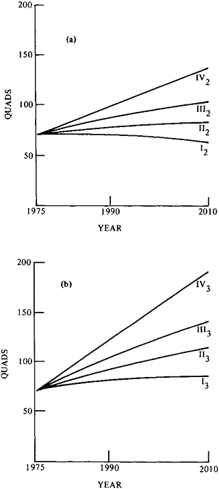
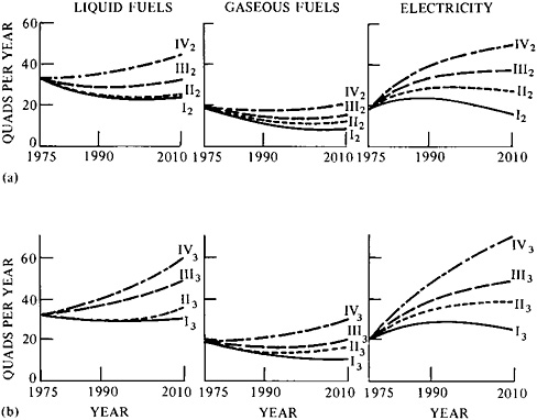
FIGURE 11–6 CONAES study scenario projections of total primary energy consumption for liquid and gaseous fuels and electricity from 1975 to 2010 (quads), with assumed (a) 2 percent GNP growth and (b) 3 percent GNP growth.
in Table 11–26. This table illustrates the sensitivity of outcomes to assumptions about electrification.
A substantial portion of the higher cost of electricity (as compared to liquid and gaseous fuels) is contributed by its capital costs. Recently, for a variety of reasons including regulations, interest rates, and construction labor costs, the capital costs of electrical generating stations have been escalating almost as rapidly as fuel costs. If, however, the capital costs of plants rose no faster than the rate of general inflation in the future, then electricity prices would rise less rapidly than primary fuel costs (which will probably continue to escalate faster than the rate of inflation). Better means of drawing on off-peak power could also contribute to greater use of electricity than indicated by the scenarios presented here. Nevertheless, the probabilities of these several possibilities are not well established,
In attempting to project the growth of demand for electricity, the electrical industry in its 1978 forecast29 speculated that lower rates of industrial production through 1995, conservation, improved near-term
TABLE 11–25 Demand for Electricity and Fluid Fuels in Study Scenarios If Half the Demand for Fluid Fuels to Supply Building Heat Is Replaced with Electrical Resistance Heat
|
Scenario |
Consumption in 1975 (quads) |
Annual Change in Demand for Electricity (percent) |
1990 (quads) |
Annual Change in Demand for Electricity (percent) |
2010 (quads) |
Generating Capacity in 2010 (gigawatts) |
|
A. Electricity |
|
|
|
|
|
|
|
I3 |
|
|
|
|
|
|
|
Base |
20 |
2.74 |
30 |
−1.32 |
23 |
460 |
|
High electricity |
— |
2.74 |
30 |
−0.43 |
27.5 |
550 |
|
II3 |
|
|
|
|
|
|
|
Base |
20 |
4.37 |
38 |
0.13 |
39 |
780 |
|
High electricity |
|
4.37 |
38 |
0.96 |
46 |
920 |
|
III3 |
|
|
|
|
|
|
|
Base |
20 |
4.55 |
39 |
1.04 |
48 |
960 |
|
High electricity |
— |
4.55 |
39 |
1.83 |
56 |
1120 |
|
IV3 |
|
|
|
|
|
|
|
Base |
20 |
7.11 |
56 |
1.60 |
71 |
1420 |
|
High electricity |
— |
7.11 |
56 |
2.23 |
87 |
1740 |
|
Scenario |
Consumption in 1975 (quads) |
1990 (quads) |
2010 (quads) |
Consumption in Buildings Sector (quads) |
|
B. Total Liquids and Gases |
||||
|
I3 |
|
|
|
|
|
Base |
53 |
50 |
42 |
(13) |
|
High electricity |
— |
50 |
38 |
(9) |
|
II3 |
|
|
|
|
|
Base |
53 |
43 |
55 |
(11) |
|
High electricity |
— |
43 |
48 |
(4) |
|
III3 |
|
|
|
|
|
Base |
53 |
57 |
67 |
(14) |
|
High electricity |
— |
57 |
58 |
(5) |
|
IV3 |
|
|
|
|
|
Base |
53 |
60 |
91 |
(27) |
|
High electricity |
— |
60 |
75 |
(11) |
TABLE 11–26 Maximum Nuclear Contribution, by Study Scenario, in High-Electricity Case Shown in Table 11–25
|
Scenario |
Primary Energy Input to Electricity Generation in 2010 (quads) |
Generating Capacity in 2010 (gigawatts) |
||
|
Total |
Nuclear |
Total |
Nuclear |
|
|
I3 |
|
|
|
|
|
Base |
23 |
6 |
460 |
120 |
|
High electricity |
27.5 |
10.5 |
550 |
210 |
|
II3 |
|
|
|
|
|
Base |
39 |
8 |
780 |
160 |
|
High electricity |
46 |
15 |
920 |
300 |
|
III3 |
|
|
|
|
|
Base |
48 |
16 |
960 |
320 |
|
High electricity |
56 |
24 |
1120 |
480 |
|
IV3 |
|
|
|
|
|
Base |
71 |
25 |
1420 |
500 |
|
High electricity |
87 |
41 |
1740 |
820 |
availability of natural gas (for residential use), and other factors will hold down the rate of growth of electricity demand. The report states,
We also hear repeated stories of greater electrification of industry, as federal and state governments cut back on industrial use of gas, and industry searches for a dependable supply of energy. This leads us to believe that fuel substitution is in fact taking place, but that it is masked by strong conservation and energy management efforts, which will become evident in the late 1980s. This change, however, is not strong enough to offset the negative elements [lower industrial production, conservation, etc.] discussed above.
One may also question the rapid price increase assumed by the Demand and Conservation Panel for natural gas. While rapid increases in the near term may be anticipated with deregulation, there is some question whether gas should be expected to command as large a premium as assumed (even in the high-price scenarios), representing up to a 12-fold increase over 1975 prices. These prices would not reflect costs of production, and there would likely be a political demand to restrict earnings on natural gas sales. On the other hand, the greater convenience and cleanliness of gas for users would fully warrant a premium over oil.
In the study scenarios, coal was assumed to be the “swing fuel” for electrical generation, filling the demand remaining after the contributions of all other fuels had been summed, The levels of coal-fired electrical
generation called for in some of the scenarios, especially by 1990, are rather high. Because of the 6–8 years required to design, construct, and license a coal-fired power plant, some of these levels could be difficult to reach. (The lead time for a nuclear power plant is even longer, by several years.)
Table 11–27 sets out the primary fuel mix for the generation of electricity in the selected study scenarios, In developing these fuel mixes, it was assumed that oil would be reserved for peaking applications, that natural gas would be phased out of the utility sector by 1990, that hydroelectric generation would grow modestly, and that solar and geothermal technologies would make small contributions by 2010, Nuclear contributions were determined from the Supply and Delivery Panel’s scenario consistent with the assumed demand policies. If electricity prices increase considerably less than assumed in the Demand and Conservation Panel’s scenarios, all these projections may underestimate the substitution of electricity for other fuels.
Liquid and Gaseous Fuels
The supply mixes of liquid and gaseous fuels for the study scenarios are shown in Table 11–28. To obtain an internally consistent supply picture (i.e., essentially equal stresses on the supply systems of oil and gas), it was necessary in scenarios II2, III2, and III3 to shift a significant amount—up to about half—of industrial-sector demand for oil to demand for gas. Without this shift, these scenarios would have called for enhanced-supply or national-commitment conditions for oil supply, but only slightly more than a business-as-usual effort to produce gas, This shift of some oil to gas is consistent with the observation of the Demand and Conservation Panel’s Industry Resource Group that gas is a preferred industrial fuel (so long as prices are competitive and supply can be assured), and that gas can be readily substituted for oil in about 50 percent of industrial use.
The numerical values for liquid and gaseous fuels in Table 11–28 include liquid fuels used for electrical generation as well as losses in the production and delivery of domestic liquids and gas, Oil and gas imports were derived as the differences between projected demand and total domestic supply under the supply conditions assumed. It is not suggested that these amounts of imports (particularly oil) will actually be available; rather, the projected needs are based on assumed supply and demand policies. In the cases of lowest growth in demand, enhanced-supply policies (especially in the area of synthetic fuel production) could replace the required imports for a given scenario.
TABLE 11–27 Primary Fuel Mix for Electricity, by Study Scenario (quads per year)a
DISCUSSION OF STUDY SCENARIOS
The study scenarios cover a wide range of potential energy supply and demand patterns (Tables 11–29 to 11–33). The totals for primary energy consumption vary widely—from 64 to 188 quads in 2010. The scenarios are even more varied in the individual components of supply and demand (as illustrated in Figures 11–7 to 11–9). The highest-consumption scenarios, for example, include contributions from light water reactors with extensive reprocessing, and from fast breeder reactors by 2010, while the lowest-consumption scenarios need only conventional light water reactors with a once-through fuel cycle and relatively small amounts of coal for electricity (Figure 11–9). Similarly, the higher-consumption scenarios entail heavy promotion of synthetic fuel production, while the low-growth scenarios require little or no synthetic fuel (Figure 11–7), The study scenarios show solar energy contributing only a small fraction to total energy consumed, with the exception of scenario I2 (about 13 percent of primary energy). A special low-energy-growth scenario developed by the Consumption, Location, and Occupational Patterns Resource Group (described previously) shows a more significant solar contribution, about 25 percent.
Characteristics of the Scenarios
High-consumption scenario IV3 (188 quads in 2010) is characterized by great expansion of nuclear power (including the introduction of breeder reactor technology as early as possible), and by aggressive exploitation of oil shale resources. This expansion would require rapid changes from current policy to encourage the development of energy resources—tax concessions, guarantees for energy investments, and expeditious processing of regulatory matters, Maintaining energy prices at essentially the levels prevailing in 1975 is unlikely to attract the capital to finance immediate expansion on all fronts. In addition, resources would have to be shifted into the development of technology to abate pollution, to protect public health and the environment, and to avert significant damage. Serious social dislocations could accompany the rapid regional shifts in economic activity implied by these scenarios.
The two medium-consumption study scenarios, III2 and III3 (102 quads and 140 quads), represent varying degrees of effort to conserve energy, spurred by policy and higher prices for energy, but they do not imply significant shifts in the mix of final purchases made by consumers. The low-consumption scenarios, CLOP and I2 (58 and 64 quads), assume changes in regional policies and in individual choices aimed at lowering energy demand. The four-times-greater prices for energy and one-thirdless consumption of energy (compared to 1975) that characterize scenario
TABLE 11–28 Liquid and Gaseous Fuel Supply Mix, by Study Scenario (quads per year)
|
Study Scenario and Energy Source |
Annual Productiona |
||
|
1975 |
1990 |
2010 |
|
|
I2 |
|
|
|
|
Domestic oil |
20 |
18 |
11 |
|
Imported oil |
13 |
5 |
12 |
|
Synthetic oil |
0 |
0 |
0 |
|
Shale oil |
0 |
0 |
0 |
|
TOTAL liquids |
33 |
23 |
23 |
|
Domestic natural gas |
19 |
13 |
8 |
|
Imported natural gas |
1 |
0 |
0 |
|
Synthetic gas |
0 |
0 |
0 |
|
TOTAL gases |
20 |
13 |
8 |
|
II2 |
|
|
|
|
Domestic oil |
20 |
18 |
11 |
|
Imported oil |
13 |
5 |
10 |
|
Synthetic oil |
0 |
0 |
4 |
|
Shale oil |
0 |
0 |
1 |
|
TOTAL liquids |
33 |
23 |
26 |
|
Domestic natural gas |
19 |
13 |
10 |
|
Imported natural gas |
1 |
0 |
3 |
|
Synthetic gas |
0 |
0 |
0 |
|
TOTAL gases |
20 |
13 |
13 |
|
III2 |
|
|
|
|
Domestic oil |
20 |
20 |
16 |
|
Imported oil |
13 |
9 |
7 |
|
Synthetic oil |
0 |
0 |
8 |
|
Shale oil |
0 |
0 |
1 |
|
TOTAL liquids |
33 |
29 |
32 |
|
Domestic natural gas |
19 |
14 |
14 |
|
Imported natural gas |
1 |
0 |
2 |
|
Synthetic gas |
0 |
0 |
0 |
|
TOTAL gases |
20 |
14 |
16 |
|
III3 |
|
|
|
|
Domestic oil |
20 |
21 |
18 |
|
Imported oil |
13 |
16 |
14 |
|
Synthetic oil |
0 |
1 |
13 |
|
Shale oil |
0 |
0 |
2 |
|
TOTAL liquids |
33 |
38 |
47 |
|
Study Scenario and Energy Source |
Annual Productiona |
||
|
1975 |
1990 |
2010 |
|
|
Domestic natural gas |
19 |
14 |
14 |
|
Imported natural gas |
1 |
1 |
1 |
|
Synthetic gas |
0 |
1 |
5 |
|
TOTAL gases |
20 |
16 |
20 |
|
IV3 |
|
|
|
|
Domestic oil |
20 |
21 |
18 |
|
Imported oil |
13 |
20 |
27 |
|
Synthetic oil |
0 |
1 |
13 |
|
Shale oil |
0 |
0 |
3 |
|
TOTAL liquids |
33 |
42 |
61 |
|
Domestic natural gas |
19 |
18 |
16 |
|
Imported natural gas |
1 |
0 |
6 |
|
Synthetic gas |
0 |
2 |
8 |
|
TOTAL gases |
20 |
20 |
30 |
|
aFigures include losses in production and distribution, but do not include conversion losses for synthetic fuels derived from coal. |
|||
I2 in 2010 would make both time and money available to deal with a lightened burden of environmental and public health consequences, but these apparent gains could be offset by the difficulties of achieving national consensus for the necessary policies and their effectuation.
Scenario II2 is driven primarily by economic changes. Its low rate of growth in energy consumption results from high energy prices (a fourfold increase) and low GNP growth (2 percent annually). However, these price levels would be considerably above production costs and would require special energy taxes, with the resulting revenue returned to the economy (e.g., through the reduction of other forms of taxation).
The midrange scenarios encompass a variety of possible energy prices (or policies) and paths for GNP. In general, the lower part of this range, scenario II3 (115 quads), presents fewer supply problems because of the slower rate of supply-system expansion (e.g., less need to change procedures for licensing and siting facilities). On the other hand, political pressures for low energy prices could present difficulties, and, of course, the economic growth assumptions are not directly subject to policy control in our models, since they depend primarily on changes in productivity.
TABLE 11–29 Projected Energy Supply and Demand in 2010 for Study Scenario I2 (quads per year)a
|
|
Demand by Energy Source |
Demand by Energy-Consuming Sector |
Totalb |
||
|
Industry |
Buildings |
Transportation |
|||
|
Liquid fuelsb |
|
8.7 |
1.6 |
10.8 |
21.1 (0.8) |
|
Domestic oil |
10.2 (0.8) |
|
|
|
|
|
Imported oil |
12 |
|
|
|
|
|
Shale oil |
0 |
|
|
|
|
|
Coal synthetics |
0 |
|
|
|
|
|
SUBTOTALc |
22.2 (0.8) |
|
|
|
|
|
Gaseous fuelsb |
|
5.8 |
1.6 |
0.1 |
7.5 (0.6) |
|
Domestic gas |
7.5 (0.6) |
|
|
|
|
|
Imported gas |
0 |
|
|
|
|
|
Coal synthetics |
0 |
|
|
|
|
|
Direct coal combustion |
|
9.4 |
0.6 |
0.1 |
10.1 |
|
Solar |
|
2.0 |
2.9 |
0 |
4.9 |
|
Other |
|
2.0 |
0 |
0 |
2.0 |
|
|
2.7 |
3.0 |
0 |
5.7 (11.3) |
|
|
Liquid fuels |
0.3 (0.8) |
|
|
|
|
|
Coal |
2.0 (3.3) |
|
|
|
|
|
Uranium in light water reactors |
1.8 (3.8) |
|
|
|
|
|
Uranium in fast breeder reactors |
0 |
|
|
|
|
|
Hydro |
1.3 (2.8) |
|
|
|
|
|
Geothermal |
0 |
|
|
|
|
|
Solar |
0.3 (0.6) |
|
|
|
|
|
TOTAL, delivered energy and losses |
|
|
|
|
51.3 (12.7) |
|
TOTAL, primary energy use |
|
|
|
|
64.0 |
|
aAssumed 2 percent average annual gross national product growth, and energy prices at 4 times 1975 prices in real dollars. bFigures in parentheses indicate the losses in production and conversion of fuels included in sectoral figures. cLiquid fuels subtotal includes liquids used directly in the buildings, industrial, and transportation sectors, and liquids used to generate electricity. dLosses in the transmission and distribution of electricity are included with purchased electricity in the values that are not in parentheses. |
|||||
Comparison with Projections of Other Energy Studies
The study scenarios are set out against scenarios of demand from other energy studies in Table 11–34. (Note that most of the projections from
TABLE 11–30 Projected Energy Supply and Demand in 2010 for Study Scenario II2 (quads per year)a
|
|
Demand by Energy Source |
Demand by Energy-Consuming Sector |
Totalb |
||
|
Industry |
Buildings |
Transportation |
|||
|
Liquid fuelsb |
|
6.5 |
2.4 |
15.1 |
24.0 (2.8) |
|
Domestic oil |
10.0 (0.8) |
|
|
|
|
|
Imported oil |
10.2 |
|
|
|
|
|
Shale oil |
0.9 |
|
|
|
|
|
Coal synthetics |
4.0 (2.0) |
|
|
|
|
|
SUBTOTALc |
25.1 (2.8) |
|
|
|
|
|
Gaseous fuelsb |
|
9.5 |
2.5 |
0.1 |
12.1 (0.7) |
|
Domestic gas |
9.1 (0.7) |
|
|
|
|
|
Imported gas |
3.0 |
|
|
|
|
|
Coal synthetics |
0 |
|
|
|
|
|
Direct coal combustion |
|
8.5 |
0 |
0.1 |
8.6 |
|
Solar |
|
1.8 |
1.6 |
0 |
3.4 |
|
Other |
|
2.7 |
0 |
0 |
2.7 |
|
|
4.6 |
5.4 |
0 |
10.0 (18.7) |
|
|
Liquid fuels |
0.3 (0.8) |
|
|
|
|
|
Coal |
5.0 (8.2) |
|
|
|
|
|
Uranium in light water reactors |
2.3 (4.8) |
|
|
|
|
|
Uranium in fast breeder reactors |
0 |
|
|
|
|
|
Hydro |
1.4 (3.0) |
|
|
|
|
|
Geothermal |
0.5 (1.3) |
|
|
|
|
|
Solar |
0.3 (0.6) |
|
|
|
|
|
TOTAL, delivered energy and losses |
|
|
|
|
60.8 (22.2) |
|
TOTAL, primary energy use |
|
|
|
|
83.0 |
|
aAssumed 2 percent average annual gross national product growth, and energy prices at 4 times 1975 prices in real dollars. bFigures in parentheses indicate the losses in production and conversion of fuels included in sectoral totals. cLiquid fuels subtotal includes liquids used directly in the buildings, industrial, and transportation sectors, and liquids used to generate electricity. dLosses in the transmission and distribution of electricity are included with purchased electricity in the values that are not in parentheses. |
|||||
other energy studies are for the year 2000, while those of CONAES are for the year 2010, A uniform basis for comparison is the column “Annual Average Rate of Growth, Energy Consumption.”) The purposes of the studies, as well as their assumptions, techniques, and accounting conven-
TABLE 11–31 Projected Energy Supply and Demand in 2010 for Study Scenario III2 (quads per year)a
|
|
Demand by Energy Source |
Demand by Energy-Consuming Sector |
Totalb |
||
|
Industry |
Buildings |
Transportation |
|||
|
Liquid fuelsb |
|
4.8 |
3.1 |
21.0 |
28.9 (5.1) |
|
Domestic oil |
14.5 (1.2) |
|
|
|
|
|
Imported oil |
7.0 |
|
|
|
|
|
Shale oil |
1.0 |
|
|
|
|
|
Coal synthetics |
8.1 (3.9) |
|
|
|
|
|
SUBTOTALc |
30.6 (5.1) |
|
|
|
|
|
Gaseous fuelsb |
|
11.5 |
3.4 |
0.1 |
15.0 (1.0) |
|
Domestic gas |
13.0 (1.0) |
|
|
|
|
|
Imported gas |
2.0 |
|
|
|
|
|
Coal synthetics |
0 |
|
|
|
|
|
Direct coal combustion |
|
10.0 |
0 |
0.1 |
10.1 |
|
Solar |
|
1.1 |
1.4 |
0 |
2.5 |
|
Other |
|
2.7 |
0 |
0 |
2.7 |
|
|
5.2 |
6.9 |
0 |
12.1 (24.6) |
|
|
Liquid fuels |
0.5 (1.2) |
|
|
|
|
|
Coal |
5.5 (10.2) |
|
|
|
|
|
Uranium in light water reactors |
4.2 (8.9) |
|
|
|
|
|
Uranium in fast breeder reactors |
— |
|
|
|
|
|
Hydro |
1.4 (3.0) |
|
|
|
|
|
Geothermal |
0.2 (0.7) |
|
|
|
|
|
Solar |
0.3 (0.6) |
|
|
|
|
|
TOTAL, delivered energy and losses |
|
|
|
|
71.3 (30.7) |
|
TOTAL, primary energy use |
|
|
|
|
102.2 |
|
aAssumed 2 percent average annual gross national product growth, and energy prices at 4 times 1975 prices in real dollars. bFigures in parentheses indicate the losses in production and conversion of fuels included in sectoral totals. cLiquid fuels subtotal includes liquids used directly in the buildings, industrial, and transportation sectors, and liquids used to generate electricity. dLosses in the transmission and distribution of electricity are included with purchased electricity in the values that are not in parentheses. |
|||||
tions, vary greatly. All these energy studies (as well as CONAES) faced the difficult problem of casting projections from slippery ground, At the time most of the projections were attempted, the equilibrium of energy and the economy had been disrupted by new prices for energy (following the oil
TABLE 11–32 Projected Energy Supply and Demand in 2010 for Study Scenario III3 (quads per year)a
|
|
Demand by Energy Source |
Demand by Energy-Consuming Sector |
Totalb |
||
|
Industry |
Buildings |
Transportation |
|||
|
Liquid fuelsb |
|
10.0 |
4.0 |
29.0 |
43.0 (7.4) |
|
Domestic oil |
16.5 (1.3) |
|
|
|
|
|
Imported oil |
14.0 |
|
|
|
|
|
Shale oil |
2.2 |
|
|
|
|
|
Coal synthetics |
13.0 (6.1) |
|
|
|
|
|
SUBTOTALc |
45.7 (7.4) |
|
|
|
|
|
Gaseous fuelsb |
|
13.9 |
4.6 |
0.2 |
18.7 (3.2) |
|
Domestic gas |
13.0 (1.0) |
|
|
|
|
|
Imported gas |
1.0 |
|
|
|
|
|
Coal synthetics |
4.7 (2.2) |
|
|
|
|
|
Direct coal combustion |
|
14.0 |
0 |
0.2 |
14.2 |
|
Solar |
|
1.1 |
1.4 |
0 |
2.5 |
|
Other |
|
3.5 |
0 |
0 |
3.5 |
|
|
6.5 |
9.5 |
0.1 |
16.1 (31.7) |
|
|
Liquid fuels |
0.8 (1.9) |
|
|
|
|
|
Coal |
7.2 (12.3) |
|
|
|
|
|
Uranium in light water reactors |
5.7 (11.8) |
|
|
|
|
|
Uranium in fast breeder reactors |
0 |
|
|
|
|
|
Hydro |
1.4 (3.0) |
|
|
|
|
|
Geothermal |
0.7 (2.1) |
|
|
|
|
|
Solar |
0.3 (0.6) |
|
|
|
|
|
TOTAL, delivered energy and losses |
|
|
|
|
98.0 (42.3) |
|
TOTAL, primary energy use |
|
|
|
|
140.3 |
|
aAssumed 2 percent average annual gross national product growth, and energy prices at 4 times 1975 prices in real dollars. bFigures in parentheses represent the losses in production and conversion of fuels included in sectoral totals. cLiquid fuels subtotal includes liquids used directly in the buildings, industrial, and transportation sectors, and liquids used to generate electricity, dLosses in the transmission and distribution of electricity are included with purchased electricity in the values that are not in parentheses. |
|||||
embargo of 1973). A decade or more may pass before these relations approach a new equilibrium. In addition, the recession of 1974–1975 induced short- and long-term changes in the economy that cannot easily be distinguished. While these differences and common difficulties warn
TABLE 11–33 Projected Energy Supply and Demand in 2010 for Study Scenario IV2 (quads per year)a
|
|
Demand by Energy Source |
Demand by Energy-Consuming Sector |
Totalb |
||
|
Industry |
Buildings |
Transportation |
|||
|
Liquid fuelsb |
|
11.9 |
6.6 |
38.6 |
57.1 (7.3) |
|
Domestic oil |
16.5 (1.3) |
|
|
|
|
|
Imported oil |
27.0 |
|
|
|
|
|
Shale oil |
3.0 |
|
|
|
|
|
Coal synthetics |
13.0 (6.0) |
|
|
|
|
|
SUBTOTALc |
59,5 (7.3) |
|
|
|
|
|
Gaseous fuelsb |
|
19.4 |
9.8 |
0.2 |
29.4 (5.2) |
|
Domestic gas |
14.8 (1.2) |
|
|
|
|
|
Imported gas |
6.4 |
|
|
|
|
|
Coal synthetics |
8.2 (4.0) |
|
|
|
|
|
Direct coal combustion |
|
13.0 |
0 |
0.2 |
13.2 |
|
Solar |
|
0.8 |
0.3 |
0 |
1.1 |
|
Other |
|
4.5 |
0 |
0 |
4.5 |
|
|
9.3 |
14.4 |
0.2 |
23.9 (47.4) |
|
|
Liquid fuels |
1.0 (2.4) |
|
|
|
|
|
Coal |
10.7 (18.2) |
|
|
|
|
|
Uranium in light water reactors |
7.6 (16.0) |
|
|
|
|
|
Uranium in fast breeder reactors |
2.0 (4.2) |
|
|
|
|
|
Hydro |
1.4 (3.0) |
|
|
|
|
|
Geothermal |
1.0 (3.0) |
|
|
|
|
|
Solar |
0.3 (0.6) |
|
|
|
|
|
TOTAL, delivered energy and losses |
|
|
|
|
129.2 (59.9) |
|
TOTAL, primary energy use |
|
|
|
|
188.1 |
|
aAssumed 2 percent average annual gross national product growth, and energy prices at 4 times 1975 prices in real dollars. bFigures in parentheses indicate the losses in production and conversion of fuels included in sectoral totals. cLiquid fuels subtotal includes liquids used directly in the buildings, industrial, and transportation sectors, and liquids used to generate electricity. dLosses in the transmission and distribution of electricity are included with purchased electricity in the values that are not in parentheses. |
|||||
against any but qualitative interpretations and comparisons, they also point up the need for continuing research into the factors that influence demand for energy, and into the several relations between energy and the
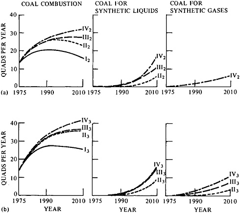
FIGURE 11–7 CONAES study scenario projections of coal consumption for combustion, synthetic liquids, and synthetic gases from 1975 to 2010 (quads), with assumed (a) 2 percent GNP growth and (b) 3 percent GNP growth.
economy (as detailed in chapter 2 under “Econometric Studies…” and “Conclusions and Recommendations”).
WORK OF THE MODELING RESOURCE GROUP
The Modeling Resource Group of the Synthesis Panel sought to compare the economic benefits and costs of various energy technologies that might be applied to meet the nation’s demand for energy over the next three decades.30 In consultation with the Risk and Impact Panel, the group found that the estimation of risks to life and health presented by various energy technologies is itself uncertain, and for some technologies, unknown. The MRG decided against attempting to reduce the estimation of these risks to a common aggregate measure (such as dollars), It reasoned that first approximations could be made for the economic costs of
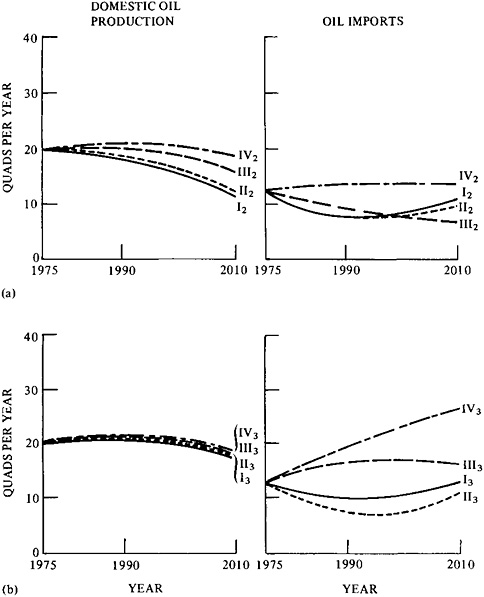
FIGURE 11–8 CONAES study scenario projections of oil consumption from domestic production and imports from 1975 to 2010 (quads), with assumed (a) 2 percent GNP growth and (b) 3 percent GNP growth.
technologies known to present some risk to human health and the environment by assuming that the use of these technologies is limited to some upper bound, and then calculating the effect on the gross national product. The loss of GNP resulting from these limitations or proscriptions represents the price of protecting the environment and human health to whatever degree is achieved with the particular assumed limits.
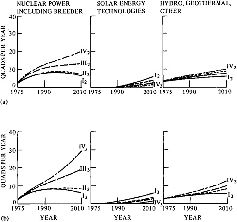
FIGURE 11–9 CONAES study scenario projections of consumption of nuclear power (including breeder); solar energy; and hydroelectric, geothermal, and other energy sources from 1975 to 2010 (quads), with assumed (a) 2 percent GNP growth and (b) 3 percent GNP growth.
Working with six large models of the domestic economy and the demand for energy, the Modeling Resource Group formalized the terms of its task as estimating the effects for outcome variables of changing certain policy variables and realization variables (as illustrated in Figure 11–10).
The realization variables selected were the following.
-
The growth rate of GNP to the year 2010 unbounded by limits or proscriptions against specific energy technologies.
-
Levels of capital cost for existing and future energy technologies.
-
The availability of oil, gas, and uranium at various costs of extraction.
-
The long-term price and income elasticities of demand for various forms of energy at the point of end-use.
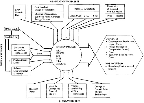
FIGURE 11–10 Compressed view of driving variables, energy models, and outcomes of the Modeling Resource Group’s work. The models vary in the detail and composition of the information inputs they require and the information outputs they produce. DRI (Data Resources, Inc., energy model) projects final demand for energy, in four principal fuels (coal, electricity, petroleum, and natural gas), and its consumption in 13 geographical regions of the United States by each of four consuming sectors (commercial, industrial, residential, and transportation). DESOM (Dynamic Energy Systems Optimization Model) assumes that demand for energy is given and determines combination of energy resources and technologies that meet this demand at least cost over time. SRI (Stanford Research Institute model) assumes that end-use demands for energy are functions of prices and simultaneously balances demands and supplies of energy for various points of an energy system (elaborated from data for 20 supply regions and 9 census regions in the United States), at particular times in a 50-yr period. PIES (Federal Energy Administration Project Independence Evaluation System), using a reference energy system, solves for the minimum-cost mix of fuels and energy technologies to meet sets of final demands. It integrates separate dynamic models of energy supply and demand to describe market equilibrium in 1980, 1985, and 1990. ETA and Nordhaus (Energy Technology Assessment model and Nordhaus simulation model) are similar to PIES, but incorporate price-sensitive energy demands, allow for consideration of a broader array of energy technologies, and project patterns of energy use further into the future. Source: Adapted from National Research Council, Supporting Paper 2: Energy Modeling for an Uncertain Future, Committee on Nuclear and Alternative Energy Systems, Synthesis Panel, Modeling Resource Group (Washington, D.C.: National Academy of Sciences, 1978), p. 9 and Appendix A.
TABLE 11–34 Energy Demand Projections by Various Studies
|
Energy Study |
Period of Projection |
Key Assumptions |
Total Energy Consumption in Final Year of Projection (quads) |
||
|
Population at End of Period (millions) |
Average Annual Rate of Growth, GNP (percent) |
Average Annual Rate of Growth, Energy Consumption (percent) |
|||
|
Ford Foundationa |
1975–2000 |
|
|
|
|
|
Historical |
|
265 |
3.02 |
3.4 |
186.7 |
|
Technical fix |
|
265 |
2.91 |
1.9 |
124.0 |
|
Zero energy growth |
|
265 |
2.92 |
1.1 |
100.0 |
|
Edison Electric Instituteb |
1975–2000 |
|
|
|
|
|
High |
|
286 |
4.2 |
3.8 |
179 |
|
Moderate |
|
265 |
3.7 |
3.2 |
155 |
|
Low |
|
251 |
2.3 |
1.6 |
105 |
|
Exxonc |
1977–1990 |
—d |
3.6 |
2.3 |
108 |
|
Bureau of Minese |
1974–2000 |
264 |
3.7 |
3.1 |
163.4 |
|
EPRIf |
1975–2000 |
|
|
|
|
|
Baselineg |
|
281 |
3.4 |
3.37 |
159 |
|
High electricityh |
|
281 |
3.4 |
4.21 |
196.1 |
|
Conservation |
|
281 |
3.4 |
2.97 |
145.6 |
|
Five times prices |
|
281 |
3.4 |
1.98 |
114.3 |
|
CONAES |
1975–2010 |
|
|
|
|
|
I2 |
|
279 |
2.0 |
–0.29 |
64 |
|
II2 |
|
279 |
2.0 |
0.45 |
83 |
|
III2 |
|
279 |
2.0 |
1.04 |
102 |
|
IV2 |
|
279 |
2.0 |
1.95 |
140 |
|
I3 |
|
279 |
3.0 |
0.52 |
85 |
|
II3 |
|
279 |
3.0 |
1.38 |
115 |
|
III3 |
|
279 |
3.0 |
1.95 |
140 |
|
IV3 |
|
279 |
3.0 |
2.82 |
188 |
|
aSource: Ford Foundation, Energy Policy Project, A Time to Choose: America’s Energy Future (Carnbridge, Mass.: Ballinger Publishing Co., 1974). bSource: Edison Electric Institute, Economic Growth in the Future, Committee on Economic Growth, Pricing and Energy Use (New York: Edison Electric Institute, 1976). cSource: Exxon Company, U.S.A., “Energy Outlook: 1978–1990,” May 1978. (Available from Public Affairs Department, P.O. Box 2180, Houston, Tex. 77001.) dNot specified. eSource: U.S. Bureau of Mines, United States Energy Through the Year 2000, rev. ed. (Washington, D.C.: U.S. Government Printing Office, 1975). fSource: Electric Power Research Institute, Demand ‘77: EPRI Annual Energy Forecasts and Consumption Model (Palo Alto, Calif.: EPRI (EA-621-SR), 1978). g With restrictions on the availability of natural gas. h With no restrictions on the availability of natural gas. |
|||||
The policy variables represent limits or proscriptions placed on the use of energy technologies.
-
A moratorium on new construction of nuclear power plants.31
-
Limits on the annual production of coal and shale oil.
In addition, the group considered “blend” variables that share the characteristics of both policy and realization variables.
-
The discount rates used to compare present values of future costs and benefits.
-
The price of oil imports, ceilings on imports, etc.
Growth Rate of Real Gross National Product
The standing of this variable as a purported measure of aggregate welfare of the population has suffered over time, and some attempts have been made to define better measures of economic welfare,32 whether by adding imputations for the services of the consumer’s capital, for the personal value of leisure, and for the value added by work done in households, or by subtracting the cost of certain negative consequences (or the cost of dealing with them), such as police services and environmental degradation.
For the MRG’s purpose of identifying a measure of aggregate economic activity that can serve as a driving variable for demand for energy, the GNP seemed as good as any other available measure of aggregate welfare, The principal question, bearing equally on all such measures, is whether the causation flows only one way, from GNP (say) to energy use, or also the other way, in the sense that direct interventions to curtail energy use would in turn have a negative effect on GNP, especially at low levels of energy availability,
Accordingly, GNP growth was classified as a realization variable, assumed to be determined over the long term by a combination of three factors largely independent of energy policy decisions: (1) population growth, (2) technological change, as reflected in labor productivity, and (3) work-force participation, The projections of GNP growth given in Table 11–35 were made by estimating potential GNP on the basis of future trends for each of these variables, assuming no more than a floor level of labor unemployment.
Over the short term, aggregate demand—not potential GNP—shapes the growth of GNP. For this reason, all estimates of GNP growth provide for higher growth over the 1975–1985 period than in subsequent periods, to account for further recovery from the recession of 1974–1975. Recessions
TABLE 11–35 Projected Growth Rate of Real Gross National Product (percent per annum)a
|
Period |
Projections |
||
|
Low |
Base Case |
High |
|
|
1975–1980 |
3.7 |
5.70 |
7.0 |
|
1980–1990 |
2.7 |
3.28 |
4.8 |
|
1990–2000 |
1.2 |
2.84 |
4.0 |
|
2000–2010 |
0.5 |
2.48 |
4.0 |
|
Beyond 2010 |
0.2 |
1.80 |
3.5 |
|
aCalculated by projecting separately three determinants of potential GNP. (Population increases by the Bureau of Census Series II projections (see Figure 11–2). Labor force participation, or ratio of actual to potential labor force (the latter equals the male and female population between 18 and 64 years of age), rises from its 1970–1975 value of 0.73 to 0.83 by 2010. Productivity. or output per worker, continues to grow from 1975 to 2000 at an average rate of 1.8 percent and grows at an average rate of 1.5 percent thereafter.) Actual GNP is assumed to complete its recovery to the level of potential GNP by 1985, and to remain equal to potential GNP after that point, at levels that ensure an average unemployment rate of 4.8 percent from 1985 through 2010. Source: Adapted from National Research Council, Supporting Paper 2: Energy Modeling for an Uncertain Future. Committee on Nuclear and Alternative Energy Systems, Synthesis Panel, Modeling Resource Group (Washington, D.C.: National Academy of Sciences, 1978), p. 13. |
|||
may, of course, recur in the future, but the Modeling Resource Group assumed GNP to remain at its potential level from 1985 on, to avoid underestimating the investments needed to meet future energy demand.
Besides the assumptions listed, the MRG’s assumption of an average annual growth rate for GNP of 3.2 percent is based on projections of public and private decisions that influence the composition of GNP, that is, allocations between investment and consumption. Should reduced energy consumption affect the amount of savings allocated to capital formation, then the growth of GNP to 2010 would follow a lower path. The MRG assumed (from empirical and conceptual considerations) that capital scarcity for investment in energy supply is unlikely.
Capital investment in the energy supply sector of the economy represented 2.64 percent of GNP in 1974. Projecting this capital investment for their various scenarios with one of the six models, the MRG noted a similar pattern. Energy-sector investment (as a percentage of GNP) drops over the near term, but returns to 1974 levels by 2010.
Feedback from Energy Use to GNP
In all MRG scenarios, GNP was treated as the principal driving variable influencing energy consumption, but not in turn influenced by it. At the same time, various scenarios considered policies that reduce energy supply, and hence consumption, directly rather than via GNP. The MRG examined the effects of policies that curtail energy supply below levels that would otherwise have prevailed—curtailments imposed for reasons of environmental protection, energy independence, or other national policy objectives. In those cases, the question naturally arose, Does the diminished use of energy also reduce GNP below what it would otherwise have been?
Virtually everyone will agree that such a reverse effect must exist. The real question is its magnitude under various circumstances. One consideration that has an important bearing on this reverse effect is discussed in chapter 2: whether the curtailment of supply is abrupt or gradual, and if abrupt, whether it is foreseen.
The models used by the Modeling Resource Group assume that the government pursues and successfully institutes a full-employment policy by maintaining aggregate demand at a level sufficient to consume whatever is produced. Thus, feedback from the contraction of energy consumption would occur only through reduction in available goods and services. If the shift to lower energy growth is a gradual one—proceeding at a rate no higher than that implicit in the normal retirement cycle of plants and equipment and in the normal turnover of labor—then capital funds and labor released from the production of energy and energy-intensive goods can find employment in other sectors.
The assumptions made about rates of capital turnover were slightly different in the six models, as detailed in the report of the MRG.33 The theoretical adjustments postulated may be inhibited by obstacles to the mobility of labor and capital. However, it appears that the adjustments necessary to accommodate long-term energy constraints or higher prices would be small compared to the adjustments required by normal technological change and differential rates of productivity growth in the economy.
Changes in energy inputs to the economy influence the pattern of capital investment over time and thus have an additional feedback effect on GNP. Reductions in energy consumption lead to changes in the rate of return on capital that alter rates of saving, investment, and the use of capital. Over time, these effects may lead to significant cumulative changes in the total capital stock, and thus in the productive capacity and output of the economy. This feedback effect can be illustrated by allowing capital to adjust to maintain a constant rate of return, rather than assuming capital and labor inputs as a constant fraction of GNP. If the elasticity of
substitution of capital for energy is 0.3, then a 50 percent reduction in energy inputs would lower GNP just 4 percent* if the capital input fraction is held constant, but would lower GNP 11 percent if capital is allowed to adjust to maintain a constant rate of return. The greater the reduction postulated, the greater the difference in effect on GNP between the two assumptions, as illustrated in Figure 11–11.34
The critical parameter that describes the quantitative effect of all energy-saving substitutions taken together, and thereby determines the feedback from energy use to GNP, is the long-term price elasticity of demand for energy. In a complete model, a matrix of price elasticities would be used to express the change in aggregate demand for each fuel in terms of the price change for each fuel. In most of the work presented here, however, this complex of effects was represented by a single price elasticity representing the ratio of the percentage change in aggregate demand for all (price-weighted) forms of primary energy to the percentage change in the average (consumption-weighted) price of primary energy. The test of the validity of this gross price elasticity would be how well the simple aggregate model, with a single primary energy, can be made to simulate the behavior of a more complex model with many fuels and many economic sectors.
Estimates of the Feedback from Energy Consumption to Real Income
Three of the models employed by the Modeling Resource Group (DESOM, ETA, and Nordhaus) minimize the discounted economic cost of meeting a set of demands for energy over a long period (subject to technological constraints and a limited range of consumer and producer behavior). In the DESOM model, the path of demand for energy is given a priori (the aggregate price elasticity of demand for primary energy is zero). In the ETA and Nordhaus models, the path of demand is obtained by maximizing the discounted sum of economic benefits to the consumer and subtracting the discounted sum of costs incurred by the producer. The optimization features of these three models enabled the MRG to estimate the economic costs (excluding those of research and development) of limiting or proscribing energy technologies in accordance with various policies. The results are displayed in Table 11–36.
Scenarios 2–6 represent alternative policies that restrict the amount of energy supplied to the economy of the United States by limiting the use of one or two energy technologies. For DESOM, the scenario entries represent the increase (over the base case) in the minimal discounted sum of year-by-
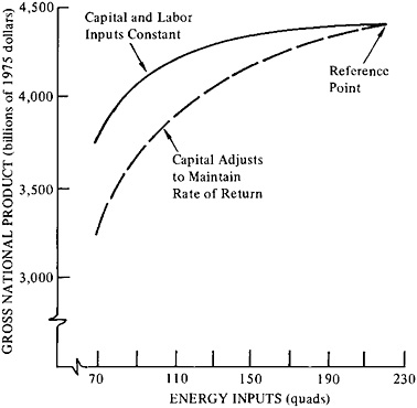
FIGURE 11–11 Effect on the economy of energy scarcity in 2010, under two alternative assumptions about capital. Source: Energy Modeling Forum, Energy and the Economy (Stanford, Calif.: Stanford University, Institute for Energy Studies, September 1977), p. 16.
year, constant-dollar costs to achieve the a priori path of demand for energy under each policy alternative. For ETA and Nordhaus, the scenario entries represent the decrease (below the base case) in the maximal discounted sum of year-by-year benefits minus costs of the paths of energy consumption in an open, competitive energy market (simulated by the same maximization). These costs (DESOM) or losses of benefits minus costs (ETA and Nordhaus) cut into the real income that might be spent for nonenergy goods and services.
The Modeling Resource Group assumed that the long-term effects of gradual and foreseeable restrictions on the supply of energy could be estimated if the percentage of total capital and labor put to work is independent of energy supply restrictions. Under that assumption. Table 11–36 can be read as discounted sums of precisely the year-by-year implications for real income of restricted energy supplies (without crediting the gains for the environment or public health). Figure 11–12 depicts the results for the ETA and Nordhaus models. The ratio set out on
TABLE 11–36 Estimated Differences in Net Economic Benefits from Six Technology Mixes and Net Economic Costs of Five Alternative Policies to Reduce Environmental Impacts (billions of 1975 dollars)
|
Policy Alternatives |
Shortfall Below Base Case of Benefits Minus Costsa |
||
|
DESOMb (Costs Only) |
ETAb |
Nordhausb |
|
|
1. Base case |
(0) |
0 |
0 |
|
2. Moratorium on all advanced converters and fast breeder reactorc |
(43) |
8 |
2 |
|
3. Moratorium on all nuclear technologies |
(105) |
46 |
136 |
|
4. Coal and shale limits |
(914) |
159 |
64 |
|
5. Moratorium on all advanced converters and fast breeder reactor, and coal and shale limits |
(1012) |
181 |
72 |
|
6. Nuclear moratorium and coal and shale limits |
(2325) |
358 |
457 |
|
aIn all policy scenarios, total benefits and costs are the sums of year-by-year benefits and costs, discounted to 1975 at 6 percent per annum. DESOM computes only discounted costs, through 2025, ETA computes discounted benefits and costs through 2050, and Nordhaus computes them through 2060. For each year, benefits estimate the value to the consumer of total amounts of energy consumed, on an incremental basis. For further explanations, see National Research Council, Supporting Paper 2: Energy Modeling for an Uncertain Future, Committee on Nuclear and Alternative Energy Systems, Synthesis Panel, Modeling Resource Group (Washington, D.C.: National Academy of Sciences, 1978), sect. III.8. bThe main features of the models used are described in the caption for Figure 11–10. cFor ETA and SRI, this policy includes a moratorium on light water reactors with plutonium recycle; for the other models it does not. |
|||
the horizontal axis is the “total energy consumption (in primary energy equivalents) for 2010 projected by scenario” to the “total energy consumption (in primary energy equivalents) for 2010 projected by the base case.” The ratio on the vertical axis is the “discounted sum of year-by-year levels of GNP minus the discounted sum of year-by-year losses in income given by scenario to the discounted sum of year-by-year levels of GNP projected by MRG.” The Modeling Resource Group concluded that the feedback effect from restrictions on energy supplies to GNP is small Apart from two points, the feedback effect is at most 2 percent of GNP, even with energy supplies restricted to 50 percent of their levels in the base case.*
There are some differences in this result among the models, and the
|
* |
See statement 11–7, by R.H.Cannon, Jr., Appendix A. |
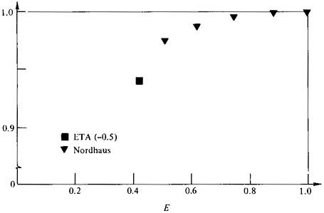
FIGURE 11–12 Estimates of the long-term feedback from aggregate energy consumption on undiscounted GNP for 2010. Nordhaus points represent policies of successive curtailments of the growth rate of energy use. Y′ on vertical axis is the ratio of undiscounted GNP in 2010 to that for the Modeling Resource Group’s base case. Source: National Research Council, Supporting Paper 2: Energy Modeling for an Uncertain Future, Committee on Nuclear and Alternative Energy Systems, Synthesis Panel, Modeling Resource Group (Washington, D.C.: National Academy of Sciences, 1978), p. 109.
Modeling Resource Group concluded that these variations could most adequately be explained by the value each assumes (explicitly or implicitly) for the price elasticity of demand (see Table 11–37).35*
Table 11–38 gives the results of assuming a “conservation tax” on energy in the ETA model that holds consumption to a constant level of 70 quads throughout the 1975–2010 period. For the Nordhaus model, as illustrated in Figure 11–12, successively more stringent limits are placed on the growth of energy consumption to achieve zero growth. Optimization determines the fuel mix at any given time in the period.
Any reduction in energy consumption that can be brought about without adding to the price reduces the conservation tax necessary to balance supply and demand, but the effects of various nonprice policies cannot be estimated from historical data. It must also be emphasized that the tax proceeds are assumed to be plowed back into the economy. If the tax were imposed, for example, by OPEC, this assumption would be violated to the extent that OPEC revenues were not offset by increased
|
* |
See statement 11–8, by R.H.Cannon, Jr., Appendix A. |
TABLE 11–37 Estimated Price and Income Elasticities of Demand for Aggregate Energy in Three Models
|
Energy Modelsa |
Elasticity of Demand for Aggregate Energy with Respect to: |
|
|
Price |
Income |
|
|
DESOM |
smallb |
0.75 |
|
ETA (price elasticity, −0.25) |
−0.25 |
1 |
|
ETA (price elasticity, −0.5) |
−0.50 |
1 |
|
Nordhaus |
0.90d |
|
|
aThe main features of the models used are described in the caption for Figure 11–10. bSince DESOM does not incorporate energy price responses by end-use consumers, its price elasticity reflects only the adjustment (small in absolute value) of the process mix between primary extraction and end use. cMade comparable to ETA price elasticities. dAverage of elasticities measured at historical 1970–1972 prices and at 2010 prices of the Nordhaus model base-case projection. Source: Adapted from National Research Council, Supporting Paper 2: Energy Modeling for an Uncertain Future, Committee on Nuclear and Alternative Energy Systems, Synthesis Panel, Modeling Resource Group (Washington, D.C.: National Academy of Sciences, 1978), p. 110. |
||
imports from the United States, and to this extent, the effect on GNP would be greater—up to the fraction of total GNP that constitutes payments for primary energy, probably not more than 5 percent
The MRG results on the size of feedback effects confirm earlier results by other investigators and add further insight into the effect of the price elasticity of demand for energy. The first feedback study based on an econometric model (to the year 2000) was made by Hudson and Jorgenson36 and was presented by the same authors37 in greater detail for the years 1980 and 1985. Using a conservation tax (referred to by the authors as a “Btu tax”), this latter effort calculated that a tax of $0.50 per million Btu in 1980, compressing total energy input by 7.8 percent, decreases GNP by only 0.42 percent, all relative to the no-tax base case.
A few differences between the assumptions underlying these estimates and those made in the applications of the ETA and Nordhaus models should be noted. The Hudson-Jorgenson (H-J) model is an equilibrium model covering the entire economy (with four nonenergy sectors and five energy sectors). This aspect of the H-J model allows a more detailed
TABLE 11–38 Estimates of the Long-Term Feedback from Aggregate Energy Consumption on Cumulative Discounted Real Gross National Producta
tracing of the effects on energy-consuming industries of a tax-induced reduction in energy use.
In comparing the conservation-tax rates of the H-J, ETA, and Nordhaus models, it should be kept in mind that in the H-J model the tax is levied on the Btu content of energy as it leaves the energy sector for use by other sectors. In the ETA and Nordhaus analyses, the tax is implicitly levied on the use of primary energy or energy equivalent. This can be read as a levy on Btu content at the point of entry into the energy-producing and energy-conversion sectors. The principal difference is that in the Modeling Resource Group’s analyses, the implicit tax on electricity is relatively much higher than in the H-J model owing to the low primary or secondary conversion efficiency of electrical generation.
In summary, the Modeling Resource Group considered only two types of policies: restricting the use of one or two energy technologies, and imposing a blanket tax on all forms of energy. It should be emphasized again that a tax on energy as such, whether on primary or ready-to-use forms, is not a suitable device for balancing the economic costs of curtailing energy use against the environmental benefits or other policy gains. Practical tax proposals to accomplish ends such as these would have to be tailored with care. The CONAES study has not investigated this issue. Qualitatively, the results would be similar to those shown for the blanket Btu or conservation tax, but would lead to a different mix of primary energy sources.
DISCUSSION
One of the puzzles emerging from the models and analyses of this study is the difference in shape of the curves projecting energy consumption over the next three decades. Those of the Demand and Conservation Panel (reflected in the curves of the study scenarios) show a considerable degree of saturation. They rise rapidly in the early part of the period 1975–2000 and level off late in the period. The curves of the Modeling Resource Group tend to be more nearly uniform over the same period.
The Demand and Conservation Panel’s results were computed from a model based on prices of net delivered energy, while those of the Modeling Resource Group were computed on the basis of the price elasticity of demand for primary energy. As the price of primary energy rises, it constitutes an increasing proportion of the price of secondary energy. A model that assumes a constant price elasticity of demand for primary energy will correspond to a model in which the price elasticity of demand for secondary energy falls as prices rise. The model of the Demand and Conservation Panel, on the other hand, corresponds to a model that assumes a constant price elasticity of demand for secondary energy. This
implies that the curves of the panel’s projections should bend more than those of the Modeling Resource Group with rising prices, and that the difference between the two will be more marked with greater assumed increases in the total price of energy.
It is difficult to make a confident choice between the two price elasticities, particularly as to which yields more realistic results.
It is important to note a factor that could make the lower-energy-growth scenarios easier to achieve than implied here. The energy conservation shown in all the scenarios is achievable by the application of known technology or of technological principles that have already been demonstrated. It does not incorporate contributions to energy efficiency from major technological innovation. Given a favorable political and economic climate for innovations in energy efficiency, substantial opportunities exist to develop and market ingenious new energy-conserving technologies. In not allowing for human ingenuity, the scenarios may understate the actual potential for moderating the consumption of energy. The ingenious use of information technologies (including microprocessors) to direct and control energy more selectively is still in its infancy and may have more potential than can now be envisaged. Such a favorable development could offset any shortfall from the conservation estimated in the scenarios, especially if energetically promoted by a combination of aggressive private marketing and highly supportive public policies.
NOTES
|
|
1. National Research Council, Supporting Paper 2: Energy Modeling for an Uncertain Future, Committee on Nuclear and Alternative Energy Systems, Synthesis Panel, Modeling Resource Group (Washington, D.C.: National Academy of Sciences, 1978). |
|
|
2. See, for example, American Gas Association, Gas Supply Review 5 (1977); National Research Council, Supporting Paper 4: Geothermal Resources and Technology in the United States, Committee on Nuclear and Alternative Energy Systems, Supply and Delivery Panel, Geothermal Resource Group (Washington, D.C.: National Academy of Sciences, 1979) and Gordon J.MacDonald, The Future of Natural Gas (McLean, Va.: Mitre Corp., 1979). |
|
|
3. See also chapter 2 of this report, and for a detailed account see National Research Council, Alternative Energy Demand Futures to 2010, Committee on Nuclear and Alternative Energy Systems, Demand and Conservation Panel (Washington, D.C.: National Academy of Sciences, 1979). |
|
|
4. Ford Foundation, Energy Policy Project, A Time to Choose: America’s Energy Future (Cambridge, Mass.: Ballinger Publishing Co., 1974). |
|
|
5. Exxon Corporation, “World Energy Outlook,” in Exxon Background Series, Public Affairs Department (New York: Exxon Corporation, April 1978), p. 7. |
|
|
6. Edison Electric Institute, Economic Growth in the Future, executive summary, Committee on Economic Growth, Pricing and Energy Use (New York: Edison Electric Institute, February 1976), p. 13. |
|
|
|
|
|
7. Institute for Energy Studies, Energy and the Economy, Energy Modeling Forum Report no. 1, vols. 1 and 2 (Stanford, Calif.: Stanford University, 1977). |
|
|
8. Demand and Conservation Panel, op. cit. |
|
|
9. Ibid., chap. 3. |
|
|
10. E.Hirst, W.Lin, and J.Cope, An Engineering-Economic Model of Residential Energy Use, (Oak Ridge, Tenn.: Oak Ridge National Laboratory (ORNL/TM-5470), July 1976); and E.Hirst et al., An Improved Engineering-Economic Model of Residential Energy Use, (Oak Ridge, Tenn.: Oak Ridge National Laboratory (ORNL/CON-8), April 1977). |
|
|
11. Demand and Conservation Panel, op. cit., chap. 3. |
|
|
12. J.R.Jackson and W.S. Johnson, Commercial Energy Use: A Disaggregation by Fuel, Building Type, and End Use (Oak Ridge, Tenn.: Oak Ridge National Laboratory (ORNL/CON-14), February 1978). |
|
|
13. J.R.Jackson, S.M.Cohn, J.Cope, and W.S.Johnson, The Commercial Demand for Energy: A Disaggregated Approach (Oak Ridge, Tenn.: Oak Ridge National Laboratory (ORNL/CON-15), April 1978). |
|
|
14. Demand and Conservation Panel, op. cit., chap. 5. |
|
|
15. For the sectoral analysis, “mass transportation” was assumed to include school buses, local and intercity buses, subways, and elevated railways. |
|
|
16. Demand and Conservation Panel, op. cit., chap. 4. |
|
|
17. Ibid., chap. 6 and app. A; see also C.W.Bullard and R.A.Herendeen, Energy Impact of Consumption Decisions (University of Illinois at Urbana: Center for Advanced Computation (CAC Document no. 135), October 1974), reprinted in Proceedings of the Institute of Electrical and Electronics Engineers 63 (March 1975):484–493. |
|
|
18. The Department of Commerce issues these data at irregular intervals. |
|
|
19. Demand and Conservation Panel, op. cit., chap. 6 and app. A. |
|
|
20. See the report of the Consumption, Location, and Occupational Patterns Resource Group of the Synthesis Panel. |
|
|
21. National Research Council, U.S. Energy Supply Prospects to 2010, Committee on Nuclear and Alternative Energy Systems, Supply and Delivery Panel (Washington, D.C.: National Academy of Sciences, 1979). |
|
|
22. Since the work of the Supply and Delivery Panel was mostly done in 1976, “existing policies” generally refer to those of that period. The effects of policy changes since that date (though not expected to be large) are generally favorable to slightly enhanced supplies. |
|
|
23. The Supply and Delivery Panel did not assess the quantitative trade-offs among supply sources implicit in this warning. |
|
|
24. National Research Council, Supporting Paper 6: Domestic Potential of Solar and Other Renewable Energy Sources, Committee on Nuclear and Alternative Energy Systems, Supply and Delivery Panel, Solar Resource Group (Washington, D.C.: National Academy of Sciences, 1979). |
|
|
25. U.S. Department of Energy, Annual Report to Congress, 1978, vol. 3, Energy Information Administration (Washington, D.C.: U.S. Department of Energy, 1979). |
|
|
26. Conservation Foundation Letter, July 1979, pp. 2–3. |
|
|
27. The study scenarios were developed by J.M.Hollander and R.Silberglitt. |
|
|
28. Edison Electric Institute, op. cit. |
|
|
29. “29th Annual Electrical Industry Forecast,” Electrical World, September 15, 1978, pp. 68–69. |
|
|
30. The Modeling Resource Group undertook two tasks. The task not described here is a systematic examination of the economic desirability of government-funded research and development of various energy technologies. See Modeling Resource Group, Supporting Paper 2, op. cit. |


