
1
High-Order, Multilevel, Adaptive Time-Domain Methods For StructuralAcoustics Simulations
J. Tinsley Oden
Andrzej Safjan
Po Geng
Leszek Demkowicz
University of Texas at Austin
|
Traditional approaches toward the computer simulation of structural acoustics phenomena have been based primarily on frequency-domain formulations of such problems, and these have dominated both the scientific literature and available analysis software in structural acoustics for many years. These classical approaches have been very successful for a limited class of problems, particularly those involving scales (wavelength) that are large relative to the characteristic dimensions of the structures. In recent times, attempts at large-scale simulations involving high ka-values have revealed limitations of many classical methods and have led to the consideration of new and alternative approaches, including time-domain techniques. This paper describes a new class of high-order methods which employ adaptive hp-version finite-element methods implemented on a special data structure designed to capture multiple-scale response. This is accomplished through the use of multilevel mesh and spectral representations, a posteriori error estimation, adaptive error control, and algorithms for treating non-reflective boundary conditions. Applications to several model problems are presented. In addition, new coupled finite-element and boundary-element methods employing frequency-domain strategies are also discussed, and comparisons with the time-domain strategies are given. |
INTRODUCTION
Much of structural acoustics is concerned with the classical problem of interaction of the motion of an elastic structure with that of a perfect inviscid fluid into which the structure is immersed. Small perturbations in the velocity or pressure fields of the fluid create waves that impinge upon the structure and scatter into the fluid-structure domain while small motions of the structure may radiate energy into
the surrounding fluid media. The radiation and scattering of waves in such fluid-structure interaction has been the subject of research for many decades.
Mathematically, the problem can be adequately modeled by a system of linear conservation laws, which, with further manipulations, can be reduced to the wave equation for the acoustical pressure coupled to the equations of elastodynamics for the structure. Traditionally, approaches for the computer simulations of structural acoustics phenomena have been primarily based on frequency-domain formulations of such problems, in which a Fourier transformation of the dynamic equations is made, and this results in a system of partial-differential equations in complex-valued field variables with frequency-dependent coefficients. The fluid may be modeled with the exterior Helmholtz equation or, as is commonly done, by an equivalent boundary-integral equation. These classical approaches have been very successful for a large and important class of problems, particularly those involving scales which are not too small in relation to characteristic dimensions of the structure. In recent times, attempts at large-scale simulations involving high ka values (k being the wave number and a the characteristic dimension) have encountered formidable computational difficulties and have exposed serious and fundamental limitations of some classical frequency-domain approaches.
In the present work, some new high-order time-domain methods are presented that have proven to be effective for simulating certain classes of problems in structural acoustics and that may have potential for overcoming many of the shortcomings of the frequency-domain methods for high ka. These techniques are built around several special ideas and algorithms:
-
the structural acoustics problem is formulated as a hyperbolic system of conservation laws and this leads to an abstract Cauchy problem in common Hilbert space settings in which the spectral theory of linear operators is applicable;
-
new, high-order, multistage Taylor-Galerkin (TG) approximations of these equations in the time-domain are constructed which deliver high-order temporal accuracy with unconditional stability;
-
spatial approximations are constructed using hp-finite element methods in which local mesh-size h and local spectral order p are varied in a way to adaptively control error, which provides multi-level approximations of the unknowns;
-
a posteriori error estimates are constructed over each element and time step to provide a running account of solution quality and to provide a basis for the adaptive control strategy;
-
applications to representative model problems reveal that the methods are robust and provide remarkably accurate results for a class of two-dimensional cases.
In addition to the time-domain methods, a brief account of a coupled boundary element/finite element method is also given. This approach also employs hp-methods and is based on a new version of the Burton-Miller integral equations for the acoustical fluid. Results obtained by using large-scale parallel computers for such problems are presented.
We also make comparisons of time-domain and frequency-domain approaches for a model class of problems. In these computations, some advantages of the time-domain approach over traditional frequency-domain approaches are observed.
A FLUID-SOLID INTERACTION PROBLEM
Statement of the Problem
Our investigation focuses on the simulation of structural acoustics phenomena using classical models of acoustics and elastic bodies characterized by systems of hyperbolic equations. The elastic structure is modeled by the classical Navier-Lamé equations of linear elasticity, and the fluid is a perfect acoustical medium modeled as a quiescent, inviscid fluid. The mathematical setting is described as follows, and is depicted in Figure 1.1.
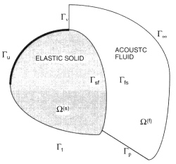
Figure 1.1 The solid-structure interaction problem.
Let ![]() be a region occupied by an elastic body and and let its boundary
be a region occupied by an elastic body and and let its boundary ![]() consist of three distinct parts,
consist of three distinct parts, ![]() where Гu and Гt are portions of
where Гu and Гt are portions of ![]() with prescribed displacements and tractions, respectively, and Гsf is the the portion of
with prescribed displacements and tractions, respectively, and Гsf is the the portion of ![]() subjected to the action of the fluid (the contact surface). Similarly, let
subjected to the action of the fluid (the contact surface). Similarly, let ![]() be a region occupied by acoustic fluid and let the boundary
be a region occupied by acoustic fluid and let the boundary ![]() consist of four distinct parts,
consist of four distinct parts, ![]() , where Гv and Гp are portions of
, where Гv and Гp are portions of ![]() with prescribed velocities and pressure, respectively,
with prescribed velocities and pressure, respectively, ![]() denotes the truncated exterior boundary, and Гfs denotes the part of the boundary which is in contact with the elastic body. We further denote Гfs = Гsf = Гc' and we use superscripts s and f to distinguish between variables having Ω(s) and Ω(f) as domains.
denotes the truncated exterior boundary, and Гfs denotes the part of the boundary which is in contact with the elastic body. We further denote Гfs = Гsf = Гc' and we use superscripts s and f to distinguish between variables having Ω(s) and Ω(f) as domains.
The fluid-solid interaction problem consists of solving:
• Equations of linear acoustics:
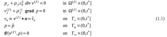
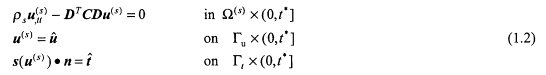
• Equations of linear elastodynamics:
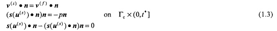
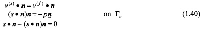
• Contact conditions:
Here:
![]() = u(s) (x,t) is the displacement vector at particle
= u(s) (x,t) is the displacement vector at particle ![]() at time t
at time t
s(u(s)) = (sij) = CDu(s) = the stress tensor evaluated at the displacement u(s)
ρs = mass density of the elastic body
C = 6 × 6 symmetric positive definite matrix of elastic constants
n = (ni) = the unit outward normal (at the interface, it is the unit outward normal to the elastic body)
p = p(x,t) is the acoustic pressure at ![]() at time t
at time t
![]() = v(f) (x,t) is the velocity in the acoustic fluid
= v(f) (x,t) is the velocity in the acoustic fluid
ρf = mass density of the acoustic fluid
c0 = small signal sound speed in the acoustic fluid
![]() = boundary operator at the truncation boundary
= boundary operator at the truncation boundary ![]()
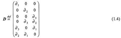
D = generalized gradient operator defined below
Problem (1.1)-(1.2) is completed by specifying initial conditions:

Here ![]() are given boundary and initial data.
are given boundary and initial data.
Equations (1.1) and (1.2) are well known, so we comment only on the interface conditions (1.3). On Гc, we have continuity of the normal component of velocity in both media, and continuity of the normal tractions. In addition, since the acoustic fluid is inviscid, we must have zero tangential traction on the elastic body on Гc.
We notice that the pressure p in (1.1) is a primitive variable which is coupled with stresses s of (1.2) through contact conditions, and the stress is not a primitive variable in (1.2). These incompatibilities prompt us to seek alternative formulations of the problem.
Velocity-Displacement Formulation
The formulation is similar to that reported in Hubert and Palencia (1989). The principal steps in the proposed methodology are as follows.
1. Introducing an auxiliary variable u(f),
and assuming the compatibility condition
equations (1.1) are transformed to the following form:
In addition, we make the usual assumption that u(f) is a potential vector field:
for some scalar field Φ.
Finally, the transition conditions (1.3) take the form
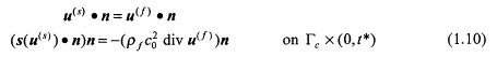
and the fluid-solid interaction problems amount to solving equations (1.2), (1.8), (1.9), (1.10).
2. Weak formulation. We now restrict attention to the case in which ![]() and
and ![]() , as indicated in Figure 1.2. Then Ω(f) and Ω(s) are assumed to be disjoint open connected sets with smooth boundaries which intersect in a C2 manifold Гc of dimension N - 1. Let u denote the displacement vector in the whole region
, as indicated in Figure 1.2. Then Ω(f) and Ω(s) are assumed to be disjoint open connected sets with smooth boundaries which intersect in a C2 manifold Гc of dimension N - 1. Let u denote the displacement vector in the whole region ![]() , and u(f) and u(s) denote, respectively, its restrictions to Ω(f) and Ω(s).
, and u(f) and u(s) denote, respectively, its restrictions to Ω(f) and Ω(s).
We start by introducing the spaces of kinematically admissible displacements

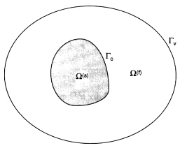
Figure 1.2 A submerged elastic structure.
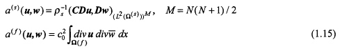
Next, we define the following Hermitian forms
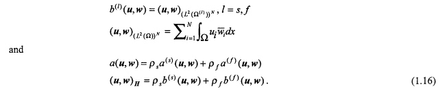
The space X, when endowed with the following inner product,
is a Hilbert space. In addition, we define space H as the completion of X with inner product (u, w)H, and, finally, we define space D(Ã) as follows

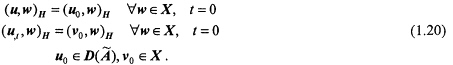
Now, we consider the following weak form of the fluid-solid interaction problem (1.2), (1.8), (1.9), (1.10):
Find ![]()
such that
and
It is easily seen that (1.19) is a classical virtual work formulation of (1.2), (1.8), (1.9), (1.10). In fact, (1.19) is valid for any test functions of appropriate regularity, not only for those of the form of gradient.
Let ![]() , where
, where ![]() denotes the space of test functions. Then (1.18) implies that (1.2) and (1.8) are satisfied in a distributional sense. Next, define a as
denotes the space of test functions. Then (1.18) implies that (1.2) and (1.8) are satisfied in a distributional sense. Next, define a as
Green's formula applied to Ω(l) and Ω(s) gives
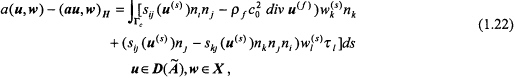
which gives transition conditions (1.10). Here n = (ni) is the unit outward normal to the elastic body and τ = (τi) is the corresponding unit outward tangent.
3. Within the above formalism, the initial boundary value problem of structural acoustics can be reinterpreted as an abstract second order Cauchy problem:
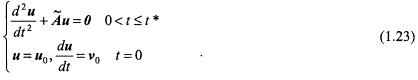
where à satisfies
u = u(t) is an H- valued function of time, and u0 and v0 are initial conditions.
To proceed further, we reinterpret (1.23) as a first-order system in time. To this end, we introduce:
• the group variable
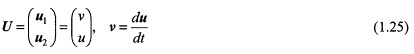
• the Hilbert space ![]()
• the operator A
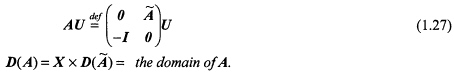
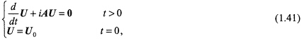
Then, (1.22) becomes:
Here U0 specifies initial conditions, ![]() .
.
To show the well-posedness of (1.28) we consider an operator ![]()
and we show that
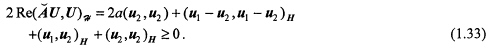
(i) ![]() is accretive, i.e.,
is accretive, i.e.,
and,
(ii) ![]() is surjective, i.e., the range of
is surjective, i.e., the range of ![]() is the whole space
is the whole space ![]()
Indeed,
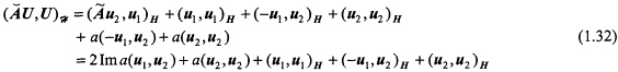
and, hence,
To prove that ![]() is surjective, we need to show that for each
is surjective, we need to show that for each ![]() there exists a solution of (A + 2I) = F, or equivalently, of the following system
there exists a solution of (A + 2I) = F, or equivalently, of the following system
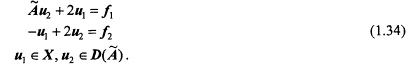
System (1.34) can be reduced to the following equation
which, by virtue of the Lax-Milgram Theorem, possesses a unique solution ![]() . This, together with (1.35) and the definition of D(Ã), implies that
. This, together with (1.35) and the definition of D(Ã), implies that ![]() . Then (1.34)2 implies that
. Then (1.34)2 implies that ![]() .
.
Summarizing, ![]() is accretive,
is accretive, ![]() is surjective, and D(A) is dense in
is surjective, and D(A) is dense in ![]() , which implies that the Cauchy problem for operator
, which implies that the Cauchy problem for operator ![]() is well posed (cf., the Lummer-Philips Theorem in Yosida, 1973). Finally, by using the ansatz
is well posed (cf., the Lummer-Philips Theorem in Yosida, 1973). Finally, by using the ansatz
we get the well posedness of (1.28). Thus, given ![]() , there exists a unique
, there exists a unique ![]() such that (1.28) is satisfied. Moreover,
such that (1.28) is satisfied. Moreover,
Problem (1.28) is to be solved numerically by using high-order Taylor-Galerkin methods and hp-adaptive finite element methods.
Velocity-Stress Formulation
The second approach consists of converting the system of equations of elastodynamics into an equivalent first-order system, and coupling it with (1.1). Thus, we solve the following first-order system. (We label it the ''velocity-stress'' formulation.)
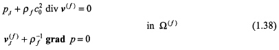
• equations of linear acoustics:
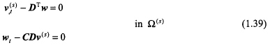
• equations of elastodynamics:
• contact conditions:
together with appropriate boundary and initial conditions. Here: ![]() , and sij are the components of the stress tensors.
, and sij are the components of the stress tensors.
As before, (1.38), (1.39), (1.40) can be cast in the form of a Cauchy problem
where U is the group variable U = (vT,wT)T, i is the imaginary unit, and A is an appropriately defined operator. Again, (1.41) is solved numerically by using high-order Taylor-Galerkin methods and hp-adaptive finite element methods.
HIGH-ORDER TAYLOR-GALERKIN (TG) METHODS
The Taylor-Galerkin (TG) schemes represent Galerkin approximations of temporal Taylor expansions of the solution. The first TG scheme was presented by Oden (1974) in connection with a Lax-Wendroff approximation of nonlinear waves by finite element methods. The TG schemes were made popular by a series of important papers by Donea and collaborators (Donea, 1984; Selmin et al., 1985), but were not applied to schemes of higher "order" than three. By a scheme of "order s" we shall understand that the one-step truncation error measured in L2 -norm is bounded by CΔts+1, where At is a time-step size and C is a constant independent of Δt. The idea of developing multi-stage high-order TG schemes was presented in the dissertation by Safjan (1993) and in subsequent papers by Safjan and Oden (1993, 1994, 1995a,b). A brief summary of the algorithm is presented below.
Let H be a Hilbert space with inner product (·,·) and corresponding norm ![]() , and
, and ![]() be a self-adjoint operator in H. Being self-adjoint, A admits the spectral decomposition of the form (Yosida, 1973)
be a self-adjoint operator in H. Being self-adjoint, A admits the spectral decomposition of the form (Yosida, 1973)
where Eλ is a uniquely defined spectral family. In this section we introduce TG schemes for solving abstract Cauchy problems of the form
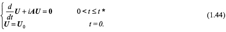
Any approximation to (1.44) must involve discretization both in space and time variables. We will adopt the assumption here that the final approximation is obtained by using finite differences in time and
finite elements in space variables. Then, two different approaches are possible. In the classical method of lines, an approximation in space variables converts the original initial-boundary-value problem into a system of ordinary differential equations (ODEs), which next is discretized in time using one of many time integration schemes for ODE.
The TG schemes belong to a different class of methods, known as themethod of discretization in time, which consists of the same two steps but done in the reverse order. By discretizing in time first, the initial-boundary-value problem (1.4) is converted into a sequence of boundary-value problems (1.45)
which, in turn, give a basis for a spatial approximation and, consequently, a fully discretized scheme,
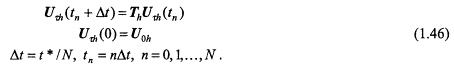
Here Uτ and Uτh are the solutions of the semi-discrete problem (1.45) and the fully discrete problem (1.46), respectively, T is an appropriate transient operator, Th denotes its finite-dimensional realization, and U0h is a suitable approximation of U0.
Approximation in Time
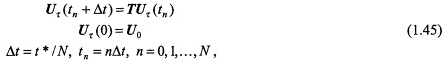
Let N be a positive integer. We define a partition in time as Δt= t */N, tn = nΔt, n = 0, 1,..., N and consider a typical time-step ![]() . Given the solution Uτ (tn), we seek the next time step solution Uτ(tn + Δt) through an s-stage scheme of the following form
. Given the solution Uτ (tn), we seek the next time step solution Uτ(tn + Δt) through an s-stage scheme of the following form
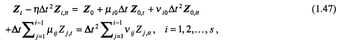
where
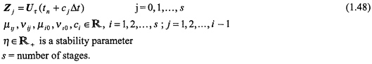
Coefficients µij, vij, µi0, vio, ci, are to be chosen so as to obtain the highest possible order of accuracy, subject to stability or other constraints. A free parameter η is to be chosen from stability considerations.
It is convenient to rewrite (1.47) in the following compact form:
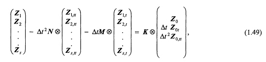
where
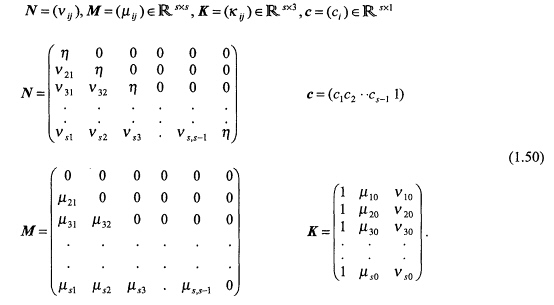
Matrices N,M, and K together with vector c completely characterize the difference scheme (1.49).
A distinct feature of (1.49) is that coefficient matrices N and M are lower triangular which makes the resulting scheme semi-implicit (i.e., to compute Zi it is necessary to know Zi-1,Zi-2,...,Z1, but it is not necessary to know Zi+1 ). Moreover, all diagonal elements of N are equal (vii = η, i = 1, 2,..., s) and so are those of M (μii = 0, i = 1, 2,..., s). This makes the operator defining the left-hand side of each stage of (1.46) identical for linear (or linearized) problems, and, hence, significantly reduces the cost of applying the method. A particular choice of zero diagonal elements of M is made with an eye on well-posedness of a typical one-stage problem and a possible splitting of the operator defining the left-hand side of each stage.
To make the i-th stage solution Zim-th order accurate, it is necessary to satisfy the order conditions for Zi and to make the previous stage solutions Zi-1,Zi-2,...,Z1, at least of the order m-1, (otherwise, some coefficients have to be set to 0; e.g., if Zi-1 is of the order m-2, then, necessarily μi,ι-1 = 0 ). The order conditions for Zi are obtained by expanding it in Taylor series about Z0:
Introducing this expression into the left-hand side of the i-th stage equation,
and equating coefficients of like powers of At to zero, leads to the following system of nonlinear algebraic equations:
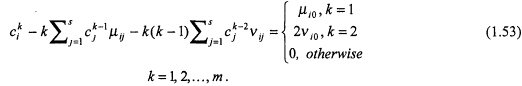
Equations (1.53) are referred to herein as the order conditions.
It is important to realize that the particular forms of the coefficient matrices M and N limit the attainable order of (direct) TG schemes. For example, it is not possible to attain order 6 in 3 stages. To remedy this situation, a more general class of transformed Taylor-Galerkin schemes has been introduced in Safjan and Oden (1994, 1995a).
Approximation in Space
First, using the original equations (1.44), we calculate the time derivatives in terms of spatial derivatives as follows:
Next, replacing the time derivatives in (1.49) by formulas (1.54) and (1.55), we arrive at the following system of equations,
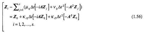
where the indices i and j are used to denote a particular stage. Finally, multiplying (1.56) by a vector-valued test function W, integrating over Ω and integrating by parts, we arrive at a variational formulation of the form:
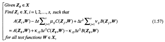
where X = D(A), and the bilinear (sesquilinear) forms A, B, and C are defined by
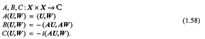
Weak form (1.57) is the basis for finite element approximations.
The properties of TG schemes are summarized as follows:
-
the TG methods lead to a series of well-posed problems that can be solved using hp-adaptive finite element methods with very high accuracy and high rates of convergence,
-
the TG methods have excellent accuracy; some of them possess a built-in temporal error estimate,
-
with a proper choice of parameters, TG methods can be unconditionally stable for certain classes of problems,
-
the TG methods can be classified as semi-implicit schemes, so that they are generally more efficient than fully implicit schemes, and provide a natural splitting of the operator that preserves accuracy, and
-
in most cases, the resulting system of linear algebraic equations is symmetric and positive definite, which is a comfortable setting for most iterative solvers.
For more details on TG schemes, we refer to Safjan and Oden (1993, 1994, 1995a,b).
HIGHLY ABSORBING BOUNDARY CONDITIONS
In many situations, we wish to solve a transient problem in an infinite domain. However, any computational domain is necessarily bounded, so it is essential to introduce appropriate boundary conditions at the boundaries. In particular, we are interested in radiating boundary conditions that have the following features:
-
the boundary conditions substantially reduce the (unphysical) reflections from the artificial boundaries,
-
the boundary conditions are local,
-
the boundary conditions together with governing differential equation result in a well-posedproblem,
-
the boundary conditions fit into the framework of our Taylor-Galerkin schemes.
We first develop radiating boundary conditions for the scalar wave equation and then deduce boundary conditions suitable for the equivalent 1st-order hyperbolic system. Our development follows Enquist and Majda (1977, 1979).
Model Problem
Let p denote the acoustical pressure and let us consider the following initial boundary-value problem for the wave equation
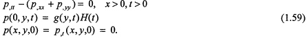
Here g(y, t) is an arbitrary square-integrable source function and H(t) is the Heaviside step function. Let δ be an acceptable error and suppose that we are interested in the solution of (1.59) in the strip ![]() , rather than in the whole right half-plane. Our objective is to find a boundary operator,
, rather than in the whole right half-plane. Our objective is to find a boundary operator, ![]() , on the wall x = a with
, on the wall x = a with ![]() , but as close to a* as possible, so that if
, but as close to a* as possible, so that if ![]() is the solution of
is the solution of
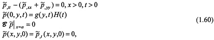
then
where time T is so large that M reflections from the artificial boundary at x = a might have occurred.
A Family of Highly Absorbing Boundary Conditions
We first derive a theoretically exact nonreflecting boundary condition. By taking the Fourier transform with respect to y and the Laplace transform with respect to t, we arrive at the following solution of (1.59):
where
ξ and ω to are dual variables to y and t, respectively, and ^ denotes the Fourier transform. We notice the correspondences ![]() and
and ![]() .
.
Let us introduce the operator ![]() which is non-local in space and time, defined by
which is non-local in space and time, defined by
Then, a simple computation reveals that the solution p satisfies the following non-local theoretical radiation condition at x = a:
By taking the Fourier transform on (1.65) we arrive at
Introducing the approximation,
(1.66) reads
By taking the inverse Fourier transform on (1.68), we get the first radiating boundary condition ![]() :
:
Using the next approximation to (1 - ξ2 / ω2)1/2:
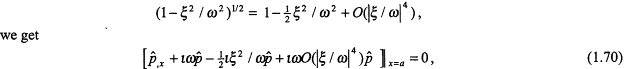
which, after taking the inverse Fourier transform, yields the boundary operator ![]() :
:
To get stable boundary operators of arbitrary order, we consider the Padé approximation to (1 - ξ2 / ω2 )1/2 of the form
Here PN (z) are recursively defined by
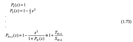
and TN+1 and SN+1 are even polynomials in z, satisfying the following relations:
Introducing (1.72) into (1.66) we get
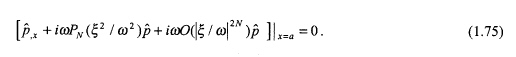
By clearing the denominator we obtain
and, observing from (1.74) that deg  and deg , we get
Using identities (1.74), it may be verified that satisfies
Finally, defining ![]() via the correspondence
via the correspondence ![]() and
and ![]() , we get
, we get
or
We now record the following fundamental result (Enquist and Majda, 1977).
-
Every
 is a local strongly well-posed boundary condition for the wave equation.
 -
Given δ, an acceptable error, a* > 0, an integer M, and an arbitrary source function satisfying
there is an ![]() and N so that if
and N so that if ![]() solves the boundary value problem in (1.60) with
solves the boundary value problem in (1.60) with ![]() then
then
for any time T with ![]() .
.
Remarks:
-
Operator
 is exact for a single space dimension and can easily be derived from physical considerations.
 -
The distance a dictating the size of computational domain, and the order of approximation N are critical parameters in practical computations.
-
Using a Taylor expansion of (1 - ξ2 / ω2 )1/2 rather than Padé approximations may result in strongly unstable boundary conditions (Enquist and Majda, 1979).
Operators and
and for Taylor-Galerkin Schemes
We first notice that wave equation (1.59) can be derived from the 1st-order system
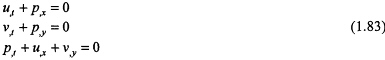
and vice versa. Here u and v denote the x- and the y-component of velocity vector, respectively, and we notice that (1.83) is nothing but the system of equations of linear acoustics in appropriately defined nondimensional variables. Then the boundary operator ![]() ,
,
can be written as
Next, assuming that the acoustic field is quiescent in the vicinity of the artificial boundary at time t = 0,
we integrate (1.85) with respect to time and obtain the following boundary condition:
Similarly, boundary operator ![]() for system (1.83) reads
for system (1.83) reads
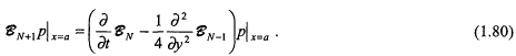
Finally, we notice that boundary operator ![]() is not easily implementable. Indeed, using recurrence relation (1.80) we compue
is not easily implementable. Indeed, using recurrence relation (1.80) we compue ![]() as
as
Next, introducing (1.83) into (1.89) and integrating with respect to time we get
Since (1.90) contains spatial derivatives of order 2, it is not acceptable for a second order operator. A new class of split boundary operators circumvents this difficulty (Safjan and Oden, 1995b).
ADAPTIVITY
In this section we give a brief outline of the hp-finite element schemes used in construction of approximation spaces ![]() .
.
First, we introduce a partition of ![]() into NELEM subdomains (elements) with disjoint interiors
into NELEM subdomains (elements) with disjoint interiors
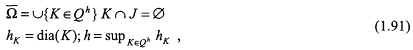
and each element K is the image of a master element ![]() under an invertible map FK,
under an invertible map FK,
On ![]() we define the following three categories of shape functions:
we define the following three categories of shape functions:
• Node functions. These are bilinear:
• Edge functions. Defining nodes at the midpoints of each side of ![]() we define the edge functions
we define the edge functions
Here ![]() is associated with side
is associated with side ![]() of
of ![]() , Δ = 1, 2, 3, 4and Φk are integrated Legendre polynomials; e.g.,
, Δ = 1, 2, 3, 4and Φk are integrated Legendre polynomials; e.g.,
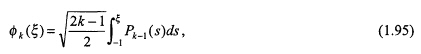
Pk-1 (s) = the Legendre polynomial of degree k - 1. Thus, polynomials of differing degree kΔ can be assigned to each edge ![]() .
.
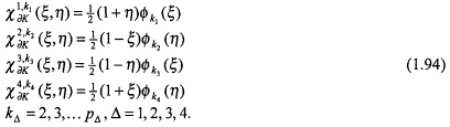
• Bubble functions. On the interior of ![]() , at its centroid, we assign the shape functions,
, at its centroid, we assign the shape functions,
Again, different orders can be assigned to different directions at (0, 0).
The master element shape functions define a space,
which, together with (1.92), define PK, a space of local shape functions for element K:
We now define Xh,p, a global finite element approximation space:
The space Xh,p possesses standard interpolation properties of hp-finite element methods (see, e.g., Babuška and Suri, 1987). In particular, for element K which is affine equivalent to a master element ![]() (i.e., TK is an affine map), if hK = dia (K) and pK is the highest degree of the complete polynomials contained in the span of shape functions associated with this element, then, for any function
(i.e., TK is an affine map), if hK = dia (K) and pK is the highest degree of the complete polynomials contained in the span of shape functions associated with this element, then, for any function ![]() , an interpolant
, an interpolant ![]() exists, such that
exists, such that
where PpK(K)= space of polynomials of degree ![]() defined on K, constant C is independent of u, pk or hk, and
defined on K, constant C is independent of u, pk or hk, and ![]() denotes the usual Sobolev norm. Then, globally, for uniform h and p, and for
denotes the usual Sobolev norm. Then, globally, for uniform h and p, and for ![]() , there exists an interpolant
, there exists an interpolant ![]() , such that
, such that
where, again, C is independent of u, p or h.
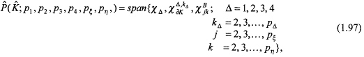
Finally, we define ![]() as
as
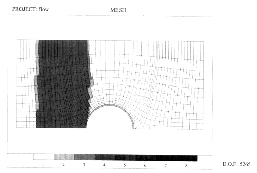
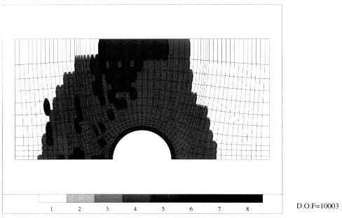
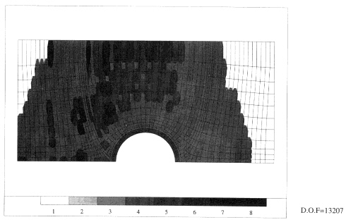
As mentioned above, (1.94) and (1.95) allow us to use shape functions of different orders for different edges (and different directions), and, hence, to construct a global mesh with a non-uniform distribution of spectral orders p. In addition, we treat mesh size h as a parameter by using h-adaptive techniques for bisecting elements and imposing hp-constraints to maintain continuity across element edges. In particular, we employ unstructured, anisotropic, 1-irregular meshes. For ![]() the mesh is composed of quadrilateral elements which are refined by dividing appropriate elements into two siblings, as opposed to four, in such a way that only one constrained node exists between any two active vertices. This provides for directional refinement whenever refinement in one direction is needed but none is called for in an orthogonal direction. An h-refined mesh of this type is depicted in Figure 1.3.
the mesh is composed of quadrilateral elements which are refined by dividing appropriate elements into two siblings, as opposed to four, in such a way that only one constrained node exists between any two active vertices. This provides for directional refinement whenever refinement in one direction is needed but none is called for in an orthogonal direction. An h-refined mesh of this type is depicted in Figure 1.3.
Continuity of global basis functions is maintained by imposing constraints at the interface of elements supporting edge functions of different order. Thus, for example, one encounters cases of the type illustrated in Figure 1.4 where an isotropic h-refinement has resulted in two small elements interfacing a large element with p-shape functions of differing order assigned to the edge (and interior) nodes. In the figure, open circles denote active vertex nodes which support bilinear shape functions, open rectangles denote edge and interior nodes which support various high-order shape functions, and darkened circles and rectangles denote constrained nodes. Thus, along the interface, values of the order of p at the p-nodes of the smaller elements (in this example) are constrained to exactly fit the shape function of the larger element to produce full continuity across this interface. For details on hp-constraints, see Demkowicz et al. (1989, 1991 a,b).
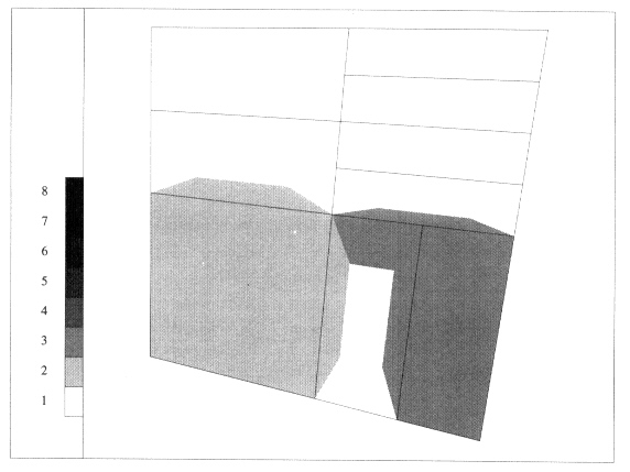
Figure 1.3 Unstructured, 1-irregular mesh of quadrilateral elements with anisotropic h-refinements. Different shadings correspond to different element spectral orders p.
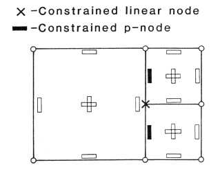
Figure 1.4 Mesh topology in two dimensions showing constrained h- and p-nodes.
A FREQUENCY-DOMAIN APPROACH
For completeness, we briefly summarize parallel work we have done on the analysis of structural acoustic problems using new coupled boundary-element and finite-element approaches in which the problem is formulated in the frequency domain.
Frequency-domain formulations are obtained by Fourier transformations of the time-domain equations and variables. For a function ![]() , its Fourier transform in time is a function û(x,ω) defined by
, its Fourier transform in time is a function û(x,ω) defined by
where ω is the frequency. We recover u(x, t) from û(x, t) by the inverse transform
Denoting the transformed displacement and pressure fields (amplitudes at the frequency co) in (1.38) and (1.39) by u(x) and p(x), respectively, we observe that a frequency-domain formulation of dynamical problem (1.27) is of the form
and
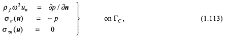
Also, the following boundary conditions must be enforced:
where k = ω / c is the wave number, Гc is the interface boundary between the interior domain Ω(s) and the exterior domain Г(f), and σn,στ, and pinc represent amplitudes of normal stress, tangential stress, and incident wave pressure at the frequency ω, respectively.
A major advantage of solving problems in the frequency-domain is that the Helmholtz equation on the exterior domain Ω(f) can be converted into an integral equation on the boundary Гc, i.e.,
In this way, the dimensionality of the problem on Ω(f) can be reduced by 1 and the infinite boundary condition (1.108) is satisfied automatically. In (1.107), Φ represents the fundamental solution of the Helmholtz equation and is of the form
and
where ![]() is the Hankel function of the first kind of 0 order and
is the Hankel function of the first kind of 0 order and ![]() .
.
As is well known, a major problem in using integral forms of the Helmholtz equation on exterior domains is that its solutions are nonunique at certain frequencies (forbidden frequencies). The CHIEF (Combined Helmholtz Integral Equation Formulation) method, proposed by Schenck (1967), is one of the earliest and simplest methods to overcome the nonuniqueness problem. In this method, the system of linear equations is combined with a few additional equations generated from the Helmholtz integral equation with the source points in the interior of the closed boundary. However, the CHIEF method is not reliable or effective in problems with complicated boundary geometry and frequencies in the higher range.
Burton and Miller (1971) proved that a complex linear combination of (1.109) and a so-called hypersingular integral equation,
is equivalent to the original differential equation. Replacing (1.106) and (1.108) by the Burton-Miller formulation leads to the following problem
Find amplitudeu = u(x)and p = p(x) such that
and
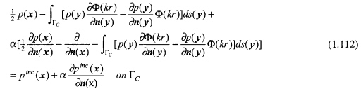
where α is a complex constant whose imaginary part cannot be 0.
Equations (1.111) through (1.113) define the mathematical model which we use to solve the acoustic scattering problem at a given frequency ω. It can be proven that the problem defined in (1.111-1.113) is strongly elliptic on the space of ![]() , and at non-resonant frequency the problem is well defined.
, and at non-resonant frequency the problem is well defined.
The Galerkin-Burton-Miller Formulation
A special problem that arises in the implementation of the Burton-Miller formulation is that the integral
in (1.112) cannot be evaluated easily in a meaningful way. Symbolically, it is customary to write (1.114) in the form
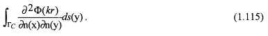
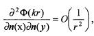
The integral kernel ![]() contains a hypersingular term and it easily verifies that as
contains a hypersingular term and it easily verifies that as ![]() in 2 dimensions
in 2 dimensions
and in 3 dimensions
Although the hypersingular integrals can be computed numerically in the sense of the finite part integral (see Kutt, 1975 and Demkowicz et al., 1991a for details), the implementation for such procedures is complicated and the accuracy of its result is usually very poor.
The method used in this study to avoid hypersingular integral kernels associated with (1.115) was proposed in Karafiat et al. (1993) and Demkowicz et al. (1992). The method requires that the problem be formulated in a weak (Galerkin) approach and is based on the transformation
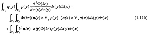
and, in 2 dimensions, this reduces to
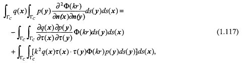
where q(x) is the test function and t(·) is the positive tangential direction at the corresponding position of x and y.
With (1.116) or (1.117), the variational formulation of (1.116)-(1.118) can be written as:
Find![]() such that for any ,
such that for any , ![]()
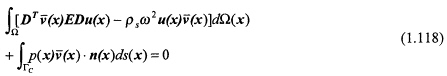
and
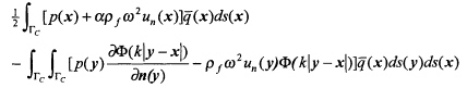
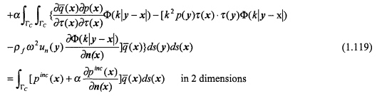
or
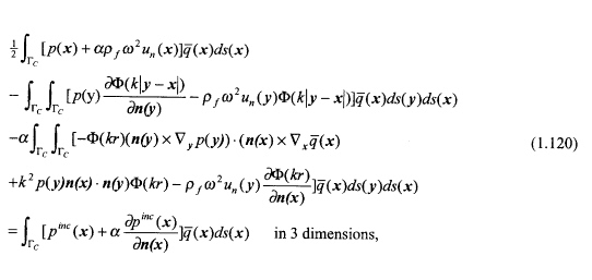
where ![]() .
.
Equations (1.119) and (1.120) contain only weak singular and regular items, which can be treated easily in numerical implementations; and the whole problem can be solved by the coupled finite element and boundary element methods.
The coupled boundary element and finite element codes in this research are developed in a special hp-hierarchical data structure proposed in Demkowicz et al. (1991b), and, as mentioned, this data structure allows the mesh size and order of polynomial interpolation to be varied over the mesh and provides a good basis for the development of an adaptive method. Comparisons with our time-domain approach are given in the next section for the elastic and rigid-scattering problems, respectively.
NUMERICAL EXAMPLES
Example 1:Diffraction of a Plane Wave from an Elastic CylindricalShell (2D)
We consider the problem of diffraction of a plane wave consisting of a short train of pulses, by an elastic shell, see Figure 1.5. The problem was solved for the following data:
Acoustic Fluid
-
Small signal sound speed, c0 = 1500 m / s
-
Ambient mass density, Pf = 7700 kg / m3
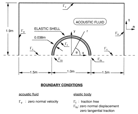
Figure 1.5 Plane progressive wave impinging on a cylindrical elastic shell. Problem definition.
Elastic Cylinder
-
Young modulus, E = 19.5 × 10¹⁰Pa,
-
Poisson's ratio, v = 0.28,
-
Mass density, Ps = 7700 kg / m3
The initial condition function:
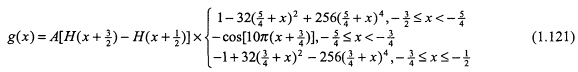
where ![]() , and A = 0.005.
, and A = 0.005.
The problem was treated as a 1st-order system, and was solved by a 2-stage 4th-order Taylor-Galerkin method with stability parameter η = 0.471 and constant time step Δt = 0.01. The solution algorithm described by Safjan and Oden (1993) was used. As the solution of the problem is fairly smooth, we chose to use p-enrichments/unenrichments only. The only exception from this rule was made in elements with contribution to the global error exceeding 50 percent; those elements were first h-refined. In addition, only p- or anisotropic h-refinements were allowed at the interface.
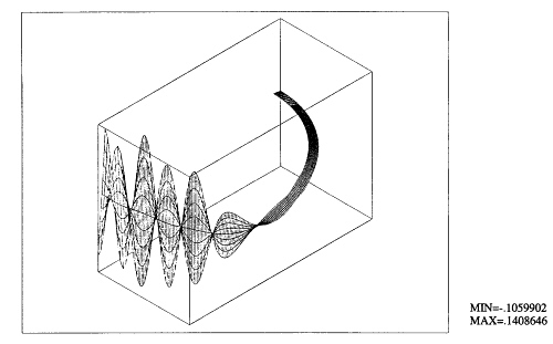
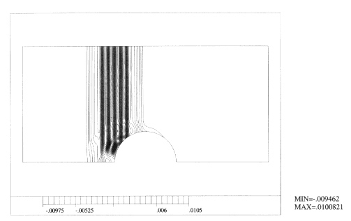
Figures 1.6 through 1.16 show the computed spatial waveforms of various acoustical and elastic variables in nondimensional form. Figure 1.6 shows the initial finite element mesh and Figure 1.7 shows the initial condition function in the form of contour maps. Figures 1.8, 1.9, and 1.10 show pressure
distribution at time t = 0.5, 1.0, and 1.5, respectively. A forward radiation from the shell can be observed, as the wave propagation speed in the shell is approximately 4 times greater than that in acoustic fluid. Figures 1.11-1.13 show the propagation of θ - θ (bending) stress waves in the elastic shell. Finally, Figures 1.14-1.16 show the evolution of finite element meshes.
Example 2:The Vibrating Cylinder Problem
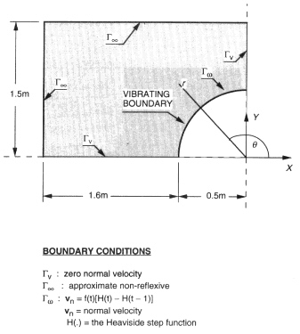
The problem is defined as follows (see Figure 1.17):
-
Governing equations of linear acoustics are to be solved in the domain

-
Boundary condition at r = a,

where A = -0.005, ω = 2π, T = 1 and H(•) is the Heaviside step function.
-
Sommerfeld radiation condition at

-
Initial condition

-
Unit material constants: c0 = 1 and Pf = 1.
For computations we accept as the computational domain ![]() and we use the second highly absorbing boundary condition
and we use the second highly absorbing boundary condition ![]() , on truncation boundary
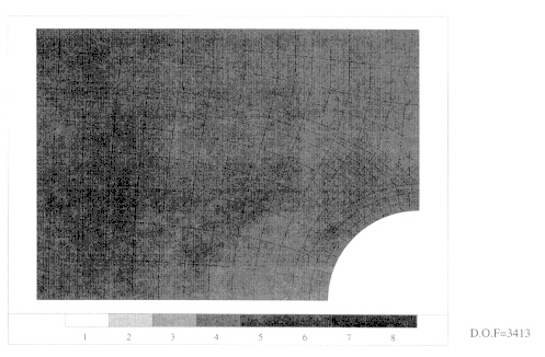
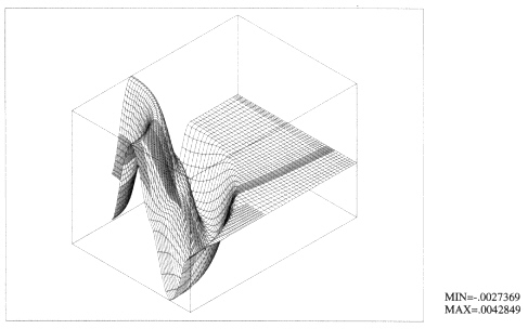
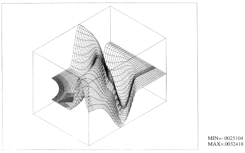
, on truncation boundary ![]() . The problem was solved using a 2-stage 4th-order Taylor-Galerkin method with stability parameter η = 0.471, constant time step Δt = 0.01, and a fixed finite element mesh. Figure 1.18 shows the finite element mesh, and the consecutive Figures 1.19, 1.20, 1.21, and 1.22 present the computed pressure distributions at time stages t = 1, 1.5, 2.0, and 2.5, respectively. As can be seen, the wave is leaving cleanly the computational domain. For comparison, the same experiment is performed except that the first highly absorbing boundary condition
. The problem was solved using a 2-stage 4th-order Taylor-Galerkin method with stability parameter η = 0.471, constant time step Δt = 0.01, and a fixed finite element mesh. Figure 1.18 shows the finite element mesh, and the consecutive Figures 1.19, 1.20, 1.21, and 1.22 present the computed pressure distributions at time stages t = 1, 1.5, 2.0, and 2.5, respectively. As can be seen, the wave is leaving cleanly the computational domain. For comparison, the same experiment is performed except that the first highly absorbing boundary condition ![]() is used on truncation boundary
is used on truncation boundary ![]() . Figure 1.23 presents the computed pressure distribution at time t = 2.5. From a comparison of the performance of
. Figure 1.23 presents the computed pressure distribution at time t = 2.5. From a comparison of the performance of ![]() with that of
with that of ![]() , it may be inferred that
, it may be inferred that ![]() represents a significant improvement over
represents a significant improvement over ![]() .
.
Example 3:The Coupled FE/BE Methods versus the Time-Domain Method
The Galerkin-Burton-Miller formulation developed here is intended to be used to solve problems at very high frequencies. To verify this, we consider an example of a harmonic plane incident wave
impinging on a cylinder with a boundary condition ![]() on the surface of the cylinder (as shown in Figure 1.24). The analytic solution is available in the case of β being a constant (Demkowicz et al., 1991b). Clearly, for β = 0, we have the problem of acoustical wave scattering on a rigid body. Figure 1.25 compares the numerical solution and corresponding analytic solution for the pressure distribution around the surface of the cylinder with ka = 400 and
on the surface of the cylinder (as shown in Figure 1.24). The analytic solution is available in the case of β being a constant (Demkowicz et al., 1991b). Clearly, for β = 0, we have the problem of acoustical wave scattering on a rigid body. Figure 1.25 compares the numerical solution and corresponding analytic solution for the pressure distribution around the surface of the cylinder with ka = 400 and ![]() . With a uniform mesh of 1,024 quadratic elements and 2,048 degrees of freedom, the result illustrated in Figure 1.25 shows a good correlation between the numerical solutions and analytic solution and the L2 -norm of relative error, computed by
. With a uniform mesh of 1,024 quadratic elements and 2,048 degrees of freedom, the result illustrated in Figure 1.25 shows a good correlation between the numerical solutions and analytic solution and the L2 -norm of relative error, computed by
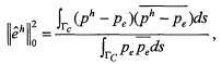
is around 2 percent in this example where Pe represents the exact solution and ph is the numerical solution.
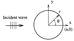
Figure 1.24 The test problem: a plane harmonic wave impinging on a cylinder.
Equations (1.105)-(1.108) define a problem of an elastic structure surrounded by an inviscid fluid field. Because of the absence of damping, the problem is not uniquely solvable at certain frequencies (resonant frequencies) and the stiffness matrix becomes singular or ill-conditioned when the frequency ω is at or close to one of these resonant frequencies.
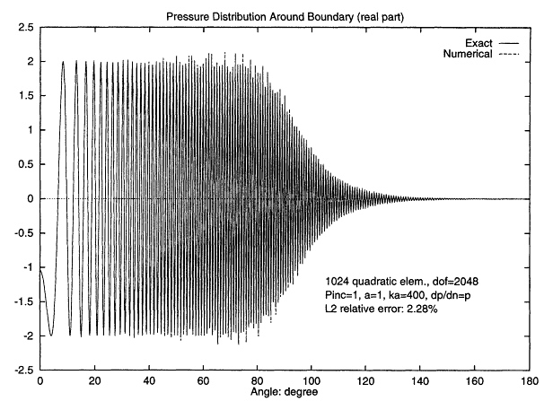
Figure 1.25 The comparison between numerical solution and analytic solution around the cylindrical boundary with ka = 400 and ![]() . Because of symmetry, only the solution from 0° to 180° around the cylindrical boundary is plotted.
. Because of symmetry, only the solution from 0° to 180° around the cylindrical boundary is plotted.
To verify this, the coupled elastic cylinder and fluid model given in Example 1 is solved for the same incident wave given in (1.125) and the wave number here varies from k = 0.02 to 14 with Δk = 0.02. A uniform mesh of 256 quadratic finite elements and 128 quadratic boundary elements is used in the computation. Figure 1.26 plots the relationship between the amplitude of total pressure at a far field point (1,0) and wave number k. The experimental results show that the test problem possesses several resonant frequencies in the range of ![]() . As a comparison, the analytic solution based on elastic thin shell theory (see Junger and Feit, 1972) is also given in Figure 1.26, and for the small wave number, the elastic solution and thin shell solution are close to each other.
. As a comparison, the analytic solution based on elastic thin shell theory (see Junger and Feit, 1972) is also given in Figure 1.26, and for the small wave number, the elastic solution and thin shell solution are close to each other.
To understand the influence of resonant frequencies on the numerical solution, the test problem given in Example 1 is solved again by the frequency-domain approach. The following incident wave is used
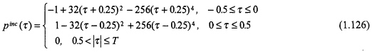
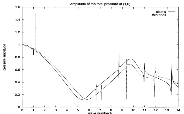
Figure 1.26 The resonant frequencies of the coupled elastic cylinder and fluid model. The plain harmonic incident wave is used and the problem is solved from k = 0.02 to k = 14 with Δk = 0.02.
where τ = x - ct and the time unit is 1/c. As shown in (1.126), the incident wave pulse must be supposed as a periodical function and T here must be large enough so that the solution at the time period in question is not affected by the solution wave from other periods. In this example, we are interested in the solution in the time period ![]() and T = 5.2 is selected. Then, the incident wave in (1.126) is decomposed into the sum of a series of sine functions, i.e.,
and T = 5.2 is selected. Then, the incident wave in (1.126) is decomposed into the sum of a series of sine functions, i.e.,
and N = 2,048. At most frequencies, pi is in fact almost zero; here, we solve the problem only at a frequency when its corresponding amplitude satisfies
Then, instead of 2,048 different frequencies, we need to solve the problem only in 124 different frequencies.
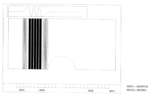
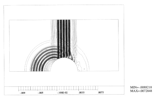
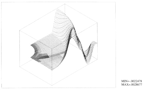
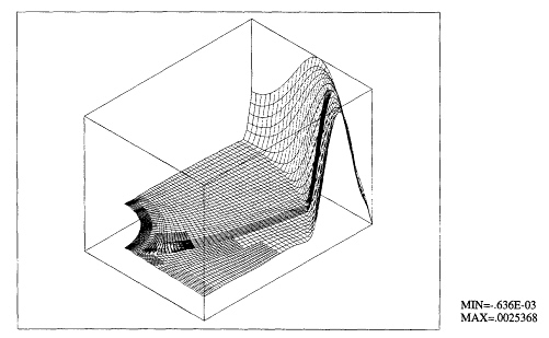
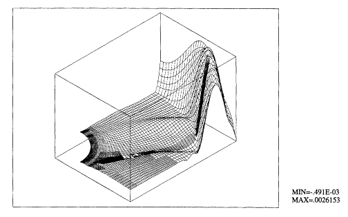
Figures 1.27 and 1.28 present the results at t = 0 and t = 2/c for the rigid scattering (![]() , upper half part) and elastic scattering (lower half part), respectively. For the rigid scattering, because the
, upper half part) and elastic scattering (lower half part), respectively. For the rigid scattering, because the
Helmholtz equation with Neumann boundary condition is well defined on the exterior domain (no resonant frequencies), the frequency-domain method produces essentially the same result obtained by the time-domain method. However, the frequency-domain method does not provide a satisfactory result for elastic scattering, because the method falls at the frequencies close to the resonant frequencies of the coupled solid-fluid system. Figure 1.27 shows spurious scattering waves produced by aliasing in the frequency-domain approach. These nonexistent waves are produced ahead of the plane wave that actually excites the structure. It is likely that these types of erroneous excitations could be controlled, if viscous and material damping effects were added to the model.
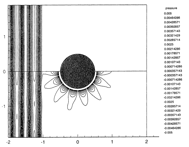
Figure 1.27 The acoustic pressure contours for the rigid scattering (upper half) and elastic scattering (lower half) at t = 0. The frequency-domain approach is used and the problem is solved in 124 different frequencies. The elastic cylinder produces spurious waves before the incident plane wave excites it.
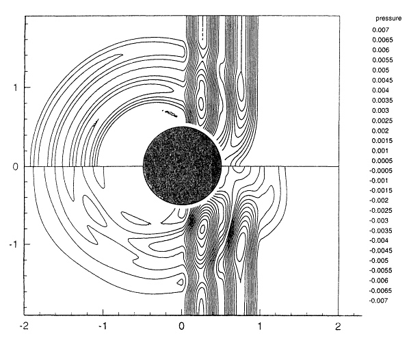
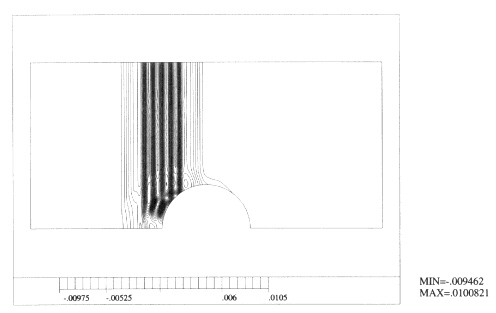
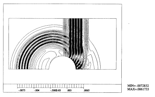
Figure 1.28 The acoustic pressure contours for the rigid scattering (upper half) and elastic scattering (lower half) at t = 2. The frequency-domain approach is used and the problem is solved in 124 different frequencies.
ACKNOWLEDGMENT
Support of this work by the Office of Naval Research (ONR) under #N00014-89-J-1451 is gratefully acknowledged.
REFERENCES
Babuška, I., and M. Suri, 1987, ''The hp version of the finite element method with quasiuniform meshes,''RAIRO Math. Model. Numer. Anal.21, 199-238.
Burton, A.J., and G.F. Miller, 1971, "The application of integral equation methods to the numerical solution of some exterior boundary-value problems,"Proc. R. Soc. London Ser.A 323,201-210.
Demkowicz, L., J.T. Oden, W. Rachowicz, and O. Hardy, 1989, "Toward a universal hp adaptive finite element strategy. part 1: constrained approximation and data structure,"Comput. Meth. Appl. Mech. Eng.77, 79-112.
Demkowicz, L., J.T. Oden, M. Ainsworth, and P. Geng,1991 a, "Solution of elastic scattering problems in linear acoustics using hp boundary element methods,"J. Comput. Appl. Math.36, 29-63.
Demkowicz, L., J.T. Oden, W. Rachowicz, and O. Hardy,1991b, "An hp Taylor-Galerkin finite method for compressible Euler equations,"Comput. Meth. Appl. Mech. Eng.88, 363-396.
Demkowicz, L., A. Karafiat, and J.T. Oden,1992, "Solution of elastic scattering problems in linear acoustics using hp boundary element method,"Comput. Meth. Appl. Mech. Eng.101, 251-282.
Donea, J., 1984, "A Taylor-Galerkin method for convective transport problems,"Int. J. Numer. Meth. Eng.88, 101-120.
Enquist, B., and A. Majda,1977, "Radiation boundary conditions for the numerical simulation of waves,"Math. Comp.31, 629-651.
Enquist, B., and A. Majda, 1979, "Radiation boundary conditions for acoustic and elastic wave calculations,"Commun. Pure Appl. Math.32, 313-357.
Hubert, J.H., and E.S. Palencia, 1989, Vibration and Coupling ofContinuous Systems, Berlin, Heidelberg, New York: Springer-Verlag.
Junger, M.C., and D. Feit,1972, Sound, Structures, and Their Interaction , Cambridge, Mass.: MIT Press.
Karafiat, A., J.T. Oden, and P. Geng, 1993, "Variational formulations and hp-boundary element approximation of hypersingular integral equations for Helmholtz-exterior boundary-value problems in two dimensions,"Int. J. Eng. Sci.31, 649-672.
Kutt, H.R., 1975, "On the numerical evaluation of finite part integrals involving an algebraic singularity,"Report WISK 179, Pretoria: The National Research Institute for Mathematical Sciences.
Oden, J.T., 1974, "Formulation and application of certain primal and mixed finite element models of finite deformations of elastic bodies." In: Computing Methods in Applied Sciences and Engineering , R. Glowinski and J.L. Lions (eds.), Berlin, Heidelberg, New York: Springer-Verlag.
Safjan, A., 1993, "High-order Taylor-Galerkin and adaptive hp methods for hyperbolic systems with application to structural acoustics,"Ph.D. Dissertation, University of Texas at Austin.
Safjan, A., and J.T. Oden, 1993, "High-order Taylor-Galerkin and adaptive hp methods for second-order hyperbolic systems: application to elastodynamics,"Comput. Meth. Appl. Mech. Eng.103, 187-230.
Safjan, A., and J.T. Oden, 1994, "High-order Taylor-Galerkin and adaptive hp methods for first-order hyperbolic systems,"TICAM Report.
Safjan, A., and J.T. Oden, 1995a, "High-order Taylor-Galerkin and adaptive hp methods for hyperbolic systems," submitted to J. Comput.Phys.
Safjan, A., and J.T. Oden, 1995b, "Highly accurate nonreflecting boundary conditions for wave propagation problems," to be submitted.
Schenck, A.H., 1967, "Improved integral formation for acoustic radiation problems,"J. Acoust. Soc. Am.44(1), 41-58.
Selmin, V., J. Donea, and L. Quartapelle, 1985, "Finite element methods for nonlinear advection,"Comput. Meth. Appl. Mech. Eng.52, 817-845.
Yosida, K., 1973, Functional Analysis, Fourth edition, Berlin, Heidelberg, New York: Springer-Verlag.


