
3
Acoustic, Elastodynamic, and Electromagnetic Wavefield Computation—AStructured Approach Based on Reciprocity
Adrianus T. de Hoop
Delft University of Technology Delft, The Netherlands
Maarten V. de Hoop
Schlumberger Cambridge Research Cambridge, England
|
The reciprocity theorems for acoustic, elastodynamic, and electromagnetic Wave fields in linear, time-invariant configurations show a common structure that can serve as a guideline for the development of computational methods for these wavefields. To this end, the wave field reciprocity theorems are taken as points of departure. They are considered to describe the "interaction" between (a discretized version of) the actual wavefield in the configuration and a suitably chosen "computational state." The choice of the computational state determines which type of computational method results from the analysis. It is shown that finite-difference/finite-element methods and integral-equation/method-of-moment methods then do arise in a natural fashion. Time-domain methods are taken as a point of departure; the relationship with complex frequency-domain methods is indicated. In the total matrix of possibilities some schemes seem as yet to be underexplored. |
INTRODUCTION
Acoustic, elastodynamic, and electromagnetic wavefields share a number of common features in their mathematical description. Their local, pointwise behavior in space-time is governed by a hyperbolic system of first-order partial differential equations that are representative for the physical phenomena involved on a local scale. When supplemented with initial conditions that relate the wave solution to its excitation mechanism and boundary conditions across interfaces where the coefficients in the system jump by finite amounts, the problem has a unique solution. The computational handling of the problem, however, often starts from a "weak" formulation, where the pointwise, or "strong," satisfaction of the equality signs in the equations is replaced by requirements on the equality of integrated or weighted
versions of the differential equations. The resulting expressions have a counterpart in physics that is found in the pertaining reciprocity theorems of the Rayleigh (acoustic waves in fluids), Betti-Rayleigh (elastic waves in solids), or H.A. Lorentz (electromagnetic waves) types. This observation has led to the approach presented in the present paper, where the relevant reciprocity theorems are taken as points of departure. Through them, a computational scheme is conceptually taken to describe the interaction between the actual wavefield state to be computed and a suitably chosen "computational state" that is representative for the method at hand, just as in physics the reciprocity theorems describe the interaction between observing state and observed state, or quantify the reciprocity between transmitting and receiving properties of any device or system (transducer in acoustics and elastodynamics, antenna in electromagnetics, electromagnetic compatibility of interfering electromagnetic systems or devices). It is also believed that through this point of view one is guided to developing computational algorithms for each of the three types of wave fields in a manner that expresses the structures common to all of them. Background literature on reciprocity can be found in some papers by A.T. de Hoop (1987, 1988, 1989, 1990, 1991, 1992) and in a forthcoming book (de Hoop, 1995).
THE BASIC FIELD EQUATIONS
We consider linear acoustic, elastic, or electromagnetic wave motion in some subdomain ![]() of three-dimensional Euclidean space
of three-dimensional Euclidean space ![]() . The configuration in which the wave motion is considered to be present is assumed to be time invariant and linear in its physical behavior. The wave quantities involved are found to satisfy certain reciprocity properties which will be taken as the point of departure for our further considerations. Now, for the indicated type of configuration, there prove to be two kinds of reciprocity theorem: one of the time-convolution type, the other of the time-correlation type. Several operations on the wave quantities will occur throughout the paper. First, we shall introduce their notation.
. The configuration in which the wave motion is considered to be present is assumed to be time invariant and linear in its physical behavior. The wave quantities involved are found to satisfy certain reciprocity properties which will be taken as the point of departure for our further considerations. Now, for the indicated type of configuration, there prove to be two kinds of reciprocity theorem: one of the time-convolution type, the other of the time-correlation type. Several operations on the wave quantities will occur throughout the paper. First, we shall introduce their notation.
Notation
Cartesian coordinates x={x1,x2,x3} are used to specify position; t is the time coordinate. Differentiation with respect to xp is denoted by ![]() is a reserved symbol for differentiation with respect to t. The subscript notation for the vectorial and tensorial quantities occurring in the wave motion will be used whenever appropriate; the subscripts are to be assigned the values 1, 2, and 3.
is a reserved symbol for differentiation with respect to t. The subscript notation for the vectorial and tensorial quantities occurring in the wave motion will be used whenever appropriate; the subscripts are to be assigned the values 1, 2, and 3.
The characteristic function of the domain ![]() is denoted by χD and is given by
is denoted by χD and is given by
where ![]() is the boundary of
is the boundary of ![]() , and
, and ![]() is the complement of
is the complement of ![]() in
in ![]()
Let F = F(x,t) denote any space-time function. Then, the time reversal operator T is defined by
It has the property
Let Q(x,t) denote another space-time function, then the time convolution Ct(F,Q) of F and Q is defined as
It has the properties
The time correlation Rt (F, Q) of F and Q is defined as
It has the properties
The First-order System of Wave Equations
Let the one-dimensional field matrix Fp = Fp(x,t) of the wave motion be composed of the components of the two wavefield quantities whose inner product represents the area density of power flow (Poynting vector). Then, Fp satisfies a system of linear, first-order, partial differential equations of the general form
where uppercase Latin subscripts are used to denote the pertaining matrix elements and the summation convention for repeated subscripts applies. In (3.12), DI,P is a symmetrical, block off-diagonal spatialdifferentiation operator matrix that contains the operator ![]() in a homogeneous linear fashion that is specific for each type of wave motion under consideration, MI,P = MI,P (x) is the medium matrix that is representative for the physical properties of the (arbitrarily inhomogeneous, anisotropic) medium in which the waves propagate, and QI = QI (x,t) is the volume source density matrix that is representative for the action of the volume sources that generate the wavefield.
in a homogeneous linear fashion that is specific for each type of wave motion under consideration, MI,P = MI,P (x) is the medium matrix that is representative for the physical properties of the (arbitrarily inhomogeneous, anisotropic) medium in which the waves propagate, and QI = QI (x,t) is the volume source density matrix that is representative for the action of the volume sources that generate the wavefield.
The medium parameters are assumed to be piecewise continuous functions of position. Across a surface of discontinuity in medium properties, the parameters may jump by finite amounts. On the assumption that the interface is passive (i.e., free from surface sources) and that the wavefield quantities
must remain bounded on either side of the interface, the wavefield must satisfy the boundary condition of the continuity type
where NI,P is the unit normal operator at the interface that arises from replacing ![]() in DI,P by np where np is the unit vector along the normal to the interface.
in DI,P by np where np is the unit vector along the normal to the interface.
For acoustic waves in fluids,
where p = acoustic pressure and vr = particle velocity, and
where q = volume source density of injection rate and fk = volume source density of force. For elastic waves in solids,
where vr = particle velocity and τp,q = dynamic stress, and
where fk = volume source density of force and hi,j = volume source density of deformation rate. For electromagnetic waves,
where Er = electric field strength and Hp = magnetic field strength, and
where Jk = volume source density of electric current and Kj = volume source density of magnetic current. The structures of DI,P and MI,P for the three types of wave fields are given in Appendix 3A.
The Reciprocity Concatenation Matrices
In the reciprocity theorems to be discussed below, two diagonal matrices ![]() and
and ![]() occur that concatenate, out of the wavefields pertaining to two admissible states, their interaction. For acoustic waves in fluids the diagonal matrix
occur that concatenate, out of the wavefields pertaining to two admissible states, their interaction. For acoustic waves in fluids the diagonal matrix ![]() is given by
is given by
for elastic waves in solids by
and for electromagnetic waves by
The diagonal matrix ![]() is just the unit matrix:
is just the unit matrix:
For the reciprocity theorem of the time-convolution type to hold, a necessary and sufficient condition proves to be
This condition requires that the block-diagonal part of DI,P be anti-symmetric and that its block off-diagonal part be symmetric. For the reciprocity theorem of the time-correlation type to hold, a necessary and sufficient condition proves to be
This condition requires that DI,P be symmetric. The two conditions are independent, but if they are satisfied simultaneously, DI,P is a symmetric, block off-diagonal matrix operator. For the three types of wave motion considered in this paper, this is indeed the case. It is therefore conjectured that the indicated structure of the spatial differential matrix operator could prove to be fundamental in order that a system of first-order partial differential equations be representative for a physical wave motion.
It is noted that the medium matrix MI,P is not subjected to any restriction of this kind.
Point-source Solutions; Green's Tensors
In view of the linearity of the wave motion, the principle of superposition ensures that the wave field Fp that is generated by the volume source distribution QI can be written as the superposition of point-source contributions through the use of a Green's tensor. The latter is a solution of the system of differential equations
where ![]() is the unit matrix and δ(x-x',t-t') is four-dimensional Dirac delta distribution operative at {x,t}= {x',t'}. In view of the time invariance of the medium, the Green's tensor depends on t and t' only through the difference t - t', i.e., GP,I' = GP,I'(x,x',t,t') = GP,I'(x,x',t - t'). The Green's tensor plays an important role in the embedding formulations of the wave field problem.
is the unit matrix and δ(x-x',t-t') is four-dimensional Dirac delta distribution operative at {x,t}= {x',t'}. In view of the time invariance of the medium, the Green's tensor depends on t and t' only through the difference t - t', i.e., GP,I' = GP,I'(x,x',t,t') = GP,I'(x,x',t - t'). The Green's tensor plays an important role in the embedding formulations of the wave field problem.
THE RECIPROCITY THEOREMS
In the wavefield reciprocity theorems certain interaction quantities are considered that are representative for the interaction between two admissible states of the pertaining wavefield in a given (proper or improper) subdomain D of ![]() . Each of the two states applies to its own medium and has its own volume source distribution. Let the superscripts A and Z indicate the two states, then the wavefields in the two states are related to their respective sources via
. Each of the two states applies to its own medium and has its own volume source distribution. Let the superscripts A and Z indicate the two states, then the wavefields in the two states are related to their respective sources via
Further, for each of the two states the boundary condition of the continuity type
holds.
The Reciprocity Theorem of the Time-convolution Type
The local interaction quantity to be considered in the reciprocity theorem of the time-convolution type is ![]() , where the property of (3.14) has been used. With the aid of (3.17) and (3.18) this expression is rewritten as
, where the property of (3.14) has been used. With the aid of (3.17) and (3.18) this expression is rewritten as
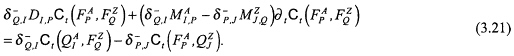
Equation (3.21) is the local form of the reciprocity theorem of the time-convolution type. The global form, for the domain ![]() , of this theorem follows upon integrating (3.21) over the domain
, of this theorem follows upon integrating (3.21) over the domain ![]() and applying Gauss' integral theorem to the first term on the left-handed side over each subdomain of
and applying Gauss' integral theorem to the first term on the left-handed side over each subdomain of ![]() where the field quantities are continuously differentiable. Adding the contributions from these subdomains, the contributions from sourcefree interfaces of discontinuity in medium properties in the interior of
where the field quantities are continuously differentiable. Adding the contributions from these subdomains, the contributions from sourcefree interfaces of discontinuity in medium properties in the interior of ![]() cancel in view of the boundary conditions given in (3.19) and (3.20) and only a surface integral over the boundary
cancel in view of the boundary conditions given in (3.19) and (3.20) and only a surface integral over the boundary ![]() of
of ![]() remains. The result is
remains. The result is
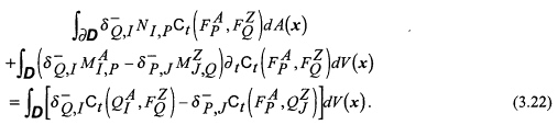
Equation (3.22) is the global form, for the domain ![]() , of the reciprocity theorem of the time-convolution type.
, of the reciprocity theorem of the time-convolution type.
The terms in (3.21) and (3.22) containing the medium matrices define the contrast-in-medium contributions to the time-convolution interaction of the two states. They vanish at those positions where ![]() . If this condition holds, the media in the two states are denoted as each other's adjoints. If the condition holds for one and the same medium, such a medium is denoted as self-adjoint. An isotropic medium is always self-adjoint. The terms containing the volume source densities yield the contribution from the volume sources to the interaction of the two states. They vanish at sourcefree positions.
. If this condition holds, the media in the two states are denoted as each other's adjoints. If the condition holds for one and the same medium, such a medium is denoted as self-adjoint. An isotropic medium is always self-adjoint. The terms containing the volume source densities yield the contribution from the volume sources to the interaction of the two states. They vanish at sourcefree positions.
In a number of applications (3.22) will be applied to the entire ![]() . Then, outside some sphere S(O, Δ0) with radius Δ0 and center at the origin O of the chosen reference frame, the media in the two states will be assumed to be the same and homogenous as well as isotropic. For such a medium, the tensor Green's function is known analytically and in particular the causal and anti-causal source-type integral representations are known analytically. For the application of (3.22) to the entire
. Then, outside some sphere S(O, Δ0) with radius Δ0 and center at the origin O of the chosen reference frame, the media in the two states will be assumed to be the same and homogenous as well as isotropic. For such a medium, the tensor Green's function is known analytically and in particular the causal and anti-causal source-type integral representations are known analytically. For the application of (3.22) to the entire ![]() , the theorem will be first applied to a sphere S(O, Δ) of radius Δ and center at the origin O of the chosen reference frame and the limit
, the theorem will be first applied to a sphere S(O, Δ) of radius Δ and center at the origin O of the chosen reference frame and the limit ![]() will be taken. If, now, in both states the wavefields are causally related to the action of their volume source distributions (assumed to have bounded supports), the integral over S(O, Δ) vanishes as
will be taken. If, now, in both states the wavefields are causally related to the action of their volume source distributions (assumed to have bounded supports), the integral over S(O, Δ) vanishes as ![]() . However, if one of the two states is causally related to the action of its volume sources and the other anti-causally, the integral over S(O,Δ) does not vanish as
. However, if one of the two states is causally related to the action of its volume sources and the other anti-causally, the integral over S(O,Δ) does not vanish as ![]() , but has a constant value for sufficiently large values of Δ.
, but has a constant value for sufficiently large values of Δ.
The Reciprocity Theorem of the Time-correlation Type
The local interaction quantity to be considered in the reciprocity theorem of the time-correlation type is ![]() , where the property of (3.15) has been used. With the aid of (3.11), (3.17), and (3.18) this expression is rewritten as
, where the property of (3.15) has been used. With the aid of (3.11), (3.17), and (3.18) this expression is rewritten as
Equation (3.23) is the local form of the reciprocity theorem of the time-correlation type. The global form, for the domain ![]() , of this theorem follows upon integrating (3.23) over the domain
, of this theorem follows upon integrating (3.23) over the domain ![]() and applying Gauss' integral theorem to the first term on the left-hand side over each subdomain of
and applying Gauss' integral theorem to the first term on the left-hand side over each subdomain of ![]() where the field quantities are continuously differentiable. Adding the contributions from these subdomains, the contributions from interfaces of discontinuity in medium properties in the interior of
where the field quantities are continuously differentiable. Adding the contributions from these subdomains, the contributions from interfaces of discontinuity in medium properties in the interior of ![]() cancel in view of the boundary conditions given in (3.19) and (3.20) and only a surface integral over the boundary
cancel in view of the boundary conditions given in (3.19) and (3.20) and only a surface integral over the boundary ![]() of
of ![]() remains. The result is
remains. The result is
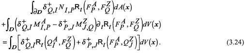
Equation (3.24) is the global form, for the domain ![]() , of the reciprocity theorem of the time-correlation type.
, of the reciprocity theorem of the time-correlation type.
The terms in (3.23) and (3.24) containing the medium matrices define the contrast-in-medium contributions to the time-correlation interaction of the two states. They vanish at those positions where ![]() . If this condition holds, the media in the two states are denoted as each other's time reverse adjoints. (The ''time-reverse'' is reminiscent of the fact that "adjoint" applies to the reciprocity theorem of the time-convolution type and that correlation can be considered as a compound operation consisting of convolution and time reversal.) If the condition holds for one and the same medium, such a medium is denoted as time-reverse self-adjoint. For an isotropic medium, the medium matrix is diagonal; an instantaneously reacting isotropic medium is therefore always time-reverse self-adjoint. The terms containing the volume source densities yield the contribution from the volume sources to the interaction of the two states. They vanish at source-free positions.
. If this condition holds, the media in the two states are denoted as each other's time reverse adjoints. (The ''time-reverse'' is reminiscent of the fact that "adjoint" applies to the reciprocity theorem of the time-convolution type and that correlation can be considered as a compound operation consisting of convolution and time reversal.) If the condition holds for one and the same medium, such a medium is denoted as time-reverse self-adjoint. For an isotropic medium, the medium matrix is diagonal; an instantaneously reacting isotropic medium is therefore always time-reverse self-adjoint. The terms containing the volume source densities yield the contribution from the volume sources to the interaction of the two states. They vanish at source-free positions.
In a number of applications (3.24) will be applied to the entire ![]() . Then, outside some sphere S(O,Δ0) with radius Δ0 and center at the origin O of the chosen reference frame, the media in the two states will be assumed to be the same and homogenous as well as isotropic. For such a medium, the tensor Green's function is known analytically and in particular the causal and anti-causal source-type integral representations are known analytically. For the application of (3.24) to the entire
. Then, outside some sphere S(O,Δ0) with radius Δ0 and center at the origin O of the chosen reference frame, the media in the two states will be assumed to be the same and homogenous as well as isotropic. For such a medium, the tensor Green's function is known analytically and in particular the causal and anti-causal source-type integral representations are known analytically. For the application of (3.24) to the entire ![]() , the theorem will be first applied to a sphere S(O, Δ) of radius Δ and center at the origin O of the chosen
, the theorem will be first applied to a sphere S(O, Δ) of radius Δ and center at the origin O of the chosen
reference frame and the limit ![]() will be taken. If, now, in State A the wave field is causally related to the action of its volume source distributions, and in State Z the wavefield is anti-causally related to the action of its volume source distributions (the volume source distributions being assumed to have bounded supports), the integral over S(O,Δ) vanishes as
will be taken. If, now, in State A the wave field is causally related to the action of its volume source distributions, and in State Z the wavefield is anti-causally related to the action of its volume source distributions (the volume source distributions being assumed to have bounded supports), the integral over S(O,Δ) vanishes as ![]() . However, if both states are causally related to the action of their volume sources, the integral over S(O,Δ) does not vanish as
. However, if both states are causally related to the action of their volume sources, the integral over S(O,Δ) does not vanish as ![]() , but has a constant value for sufficiently large values of Δ.
, but has a constant value for sufficiently large values of Δ.
For the choice State A = State Z and zero correlation time shift (i.e., t = 0), (3.23) reduces to the local energy balance for the wavefield and (3.24) to the global energy balance for the domain ![]() , provided that MQ.P = MP,Q. This implies that for the energy considerations pertaining to a physical wavefield to hold, the medium matrix must be symmetric. In that case, also the quantity (1/2)MP.QFPFQ (whose time derivative occurs in equations (3.23) and (3.24)) should represent the volume density of stored energy. For the latter, the symmetric medium matrix should, in addition, on physical grounds be positive definite.
, provided that MQ.P = MP,Q. This implies that for the energy considerations pertaining to a physical wavefield to hold, the medium matrix must be symmetric. In that case, also the quantity (1/2)MP.QFPFQ (whose time derivative occurs in equations (3.23) and (3.24)) should represent the volume density of stored energy. For the latter, the symmetric medium matrix should, in addition, on physical grounds be positive definite.
Reciprocity Property of the Causal Green's Tensor
Equation (3.22) leads to a reciprocity property of the Green's tensor. Let ![]() be the causal wavefield in Medium A generated by the point source
be the causal wavefield in Medium A generated by the point source ![]() operative at {x,t} = {x',0}. Then (cf. (3.16))
operative at {x,t} = {x',0}. Then (cf. (3.16)) ![]() . Let, similarly,
. Let, similarly, ![]() be the causal wavefield in Medium Z generated by the point source
be the causal wavefield in Medium Z generated by the point source ![]() operative at {x,t} = {x",0}. Then
operative at {x,t} = {x",0}. Then ![]() . Take the media in the two states as each other's adjoints, i.e.,
. Take the media in the two states as each other's adjoints, i.e., ![]() , and apply (3.22) to the entire
, and apply (3.22) to the entire ![]() . In this application, the contrast-in-media term and the contribution from the "sphere at infinity" vanish. The result is
. In this application, the contrast-in-media term and the contribution from the "sphere at infinity" vanish. The result is
Since (3.25) has to hold for arbitrary values of ![]() and
and ![]() we end up with
we end up with
Equation (3.26) is the reciprocity relation for the causal Green's tensor.
EMBEDDING PROCEDURE, CONTRAST-PROPERTIES FORMULATION
On many occasions the wavefield computation in an entire configuration is beyond the capabilities because of the storage capacity required and the computation time involved. In that case, it is standard practice to select a target region ![]() of bounded support in which a detailed computation is to be
of bounded support in which a detailed computation is to be
carried out, while the medium in the remaining part of the configuration (the embedding) is chosen to be so simple that the wave motion in it can be determined with the aid of analytical methods. In particular, this applies to scattering problems and to geophysical modeling, where the support of the model configuration is often taken to be the entire ![]() . Examples of such simple embeddings are a homogeneous, isotropic medium (chosen for most scattering configurations) and a medium consisting of parallel layers of homogeneous, isotropic material (chosen in most geophysical applications). In these cases, time Laplace and spatial Fourier transform techniques provide the analytical tools to determine the wave motion or, in fact, the relevant Green's tensor. Once the embedding has been chosen, the problem of computing the wavefield in
. Examples of such simple embeddings are a homogeneous, isotropic medium (chosen for most scattering configurations) and a medium consisting of parallel layers of homogeneous, isotropic material (chosen in most geophysical applications). In these cases, time Laplace and spatial Fourier transform techniques provide the analytical tools to determine the wave motion or, in fact, the relevant Green's tensor. Once the embedding has been chosen, the problem of computing the wavefield in ![]() can be formulated as a contrast problem . For this, we proceed as follows.
can be formulated as a contrast problem . For this, we proceed as follows.
The State A is introduced consisting of the Actual wavefield ![]() , the actual sources
, the actual sources ![]() that excite it, and the actual medium
that excite it, and the actual medium ![]() in which the propagation takes place. Next, we introduce a State B consisting of the wavefield
in which the propagation takes place. Next, we introduce a State B consisting of the wavefield ![]() that the actual sources
that the actual sources ![]() would generate in the medium
would generate in the medium ![]() of the emBedding. Denoting the Green's tensor of the embedding by
of the emBedding. Denoting the Green's tensor of the embedding by ![]() the latter wavefield is expressible as
the latter wavefield is expressible as
where ![]() is the support of the sources that generate the wavefield in the actual configuration. From the corresponding wavefield equations it then follows that
is the support of the sources that generate the wavefield in the actual configuration. From the corresponding wavefield equations it then follows that
This equation can be rewritten in two ways as a wavefield equation for the Contrast state, to be denoted by the superscript C, in which the contrast wave field is
In one of them, the medium properties in the wave operator on the left-hand side are taken to be the ones of the actual medium; this is typically done in the combination of the embedding technique with finite-element or finite-difference modeling. In the other, the medium properties in the wave operator on the left-hand side are taken to be the ones of the embedding; this is typically done in the integral-equation or method-of-moments modeling. Both ways lead to a contrast-source formulation. The expressions for the two cases are given below.
Contrast Formulation for Finite-element/Finite-difference Modeling
For the contrast formulation for finite-element or finite-difference modeling, (3.28) is, in combination with (3.29), rewritten as
with
and
Note that in this contrast formulation, the contrast source density ![]() is known.
is known.
Contrast Formulation for Integral-equation/Method-of-Moments Modeling
For the contrast formulation for integral-equation or methods-of-moments modeling, (3.28) is, in combination with (3.29), rewritten as
with
and
Note that in this contrast formulation, the contrast source density ![]() is unknown, since
is unknown, since ![]() is unknown.
is unknown.
In the two sections following, it will be indicated how these different states are used in the reciprocity theorems of the previous section to lead to computational schemes for the evaluation of the wavefields.
FINITE-ELEMENT/FINITE-DIFFERENCE MODELING
In finite-element/finite-difference modeling over an entire configuration occupying the bounded domain ![]() , the wavefield to be computed is the total wavefield. The latter is approximated by an expansion of the type
, the wavefield to be computed is the total wavefield. The latter is approximated by an expansion of the type
where ![]() is an appropriate sequence of known, linearly independent expansion functions with
is an appropriate sequence of known, linearly independent expansion functions with ![]() as their supports, and
as their supports, and ![]() is the sequence of expansion coefficients to be computed. In typical finite-element/finite-difference modeling the support of each expansion function is an elementary subdomain of the (discretized) version of
is the sequence of expansion coefficients to be computed. In typical finite-element/finite-difference modeling the support of each expansion function is an elementary subdomain of the (discretized) version of ![]() (usually a simplex or a complex). Further, boundary conditions as needed for the uniqueness of the solution in
(usually a simplex or a complex). Further, boundary conditions as needed for the uniqueness of the solution in ![]() are prescribed on
are prescribed on ![]() . Next, a sequence of "computational" states, denoted by the superscript Z, is selected, for which
. Next, a sequence of "computational" states, denoted by the superscript Z, is selected, for which
where the right-hand side is a sequence of known, linearly independent weighting functions with ![]() as their supports. Finally, we take
as their supports. Finally, we take
and hence
Application of the earlier reciprocity theorems to the State A and the sequence of States Z leads to a system of linear algebraic equations in the expansion coefficients.
Embedding Procedure
In case an embedding procedure is applied, the wavefield to be computed is the contrast wavefield. The latter is approximated by an expansion of the type
where ![]() is an appropriate sequence of known, linearly independent expansion functions with
is an appropriate sequence of known, linearly independent expansion functions with ![]() as their supports and
as their supports and ![]() is now the sequence of expansion coefficients to be computed. In typical finite-element/finite-difference modeling the support of each expansion function is an elementary subdomain of the (discretized) version of
is now the sequence of expansion coefficients to be computed. In typical finite-element/finite-difference modeling the support of each expansion function is an elementary subdomain of the (discretized) version of ![]() (usually a simplex or a complex). Further, "absorbing boundary conditions" as needed for the uniqueness of the solution in
(usually a simplex or a complex). Further, "absorbing boundary conditions" as needed for the uniqueness of the solution in ![]() are prescribed on
are prescribed on ![]() . These should model the radiation of the contrast wavefield into the passive embedding. Next, a sequence of "computational" states, denoted by the superscript Z, is selected, for which
. These should model the radiation of the contrast wavefield into the passive embedding. Next, a sequence of "computational" states, denoted by the superscript Z, is selected, for which
where the right-hand side is a sequence of known, linearly independent weighting functions with ![]() as their supports. Finally, we take
as their supports. Finally, we take
and hence
Application of the reciprocity theorems to the State A and the sequence of States Z again leads to a system of linear algebraic equations in the expansion coefficients.
In finite-element/finite-difference modeling, the expansion and weighting functions are standardly taken to be polynomials in the time variable and the spatial variables. Their vector and tensor components in space can be organized such that the continuity conditions across an interface between two different media are taken into account automatically, while leaving those components that are not necessarily continuous free to jump by finite amounts. Such a procedure can be carried out consistently if the simplex is taken as the elementary subdomain of the discretized configuration and a consistent linear approximation within each simplex is used. Thus, the notions of "face element" and "edge element" for arbitrary vectors and tensors have been introduced. For literature on the subject, see Mur and de Hoop (1985) and Mur (1990, 1991, 1993) for the application to electromagnetic fields and Stam and de Hoop (1988, 1989, 1990) for the application to elastodynamic wavefields.
METHOD-OF-MOMENTS MODELING
The integral-equation or method-of-moments modeling is invariably based on an embedding procedure. As a consequence of this, the wavefield to be computed is the contrast wavefield. The latter is approximated by
where ![]() is an appropriate sequence of known, linearly independent expansion functions with
is an appropriate sequence of known, linearly independent expansion functions with ![]() as their supports, and
as their supports, and ![]() is the sequence of expansion coefficients to be computed. The contrast source density is written as
is the sequence of expansion coefficients to be computed. The contrast source density is written as
in which the first term on the right-hand side is known and the second term on the fight-hand side is unknown. Next, a "computational" state, denoted by the superscript Z, is selected, for which
and
Substitution in the earlier reciprocity theorems then leads to a system of linear, algebraic equations in the expansions coefficients.
COMPLEX FREQUENCY-DOMAIN MODELING OF WAVE PROBLEMS
Although the real, physical wave phenomena take place in space-time, it can under certain circumstances be advantageous to parametrize the problem in the coordinates in which shift invariance in the configuration occurs. Since we have assumed that our configurations are, apart from linear, time-invariant in their physical behavior, such a procedure certainly applies to the time coordinate. Moreover, in this coordinate the principle of causality applies. In view of these two aspects, the time Laplace transformation performs the appropriate parametrization in the time coordinate. For any causal, bounded function QI = QI(x,t) with temporal support ![]() this transformation is
this transformation is
Here, s is the time Laplace transform parameter or complex frequency. The time Laplace transformation has the following properties:
In view of Lerch's theorem (Widder, 1946), the correspondence between ![]() and QI(x,t) for t>t0 is unique. Using these properties, the space-time wave motion can be recovered after having solved a sequence of space problems with appropriate values of the time Laplace transform parameter. For recent results in this direction, see Lee et al. (1994).
and QI(x,t) for t>t0 is unique. Using these properties, the space-time wave motion can be recovered after having solved a sequence of space problems with appropriate values of the time Laplace transform parameter. For recent results in this direction, see Lee et al. (1994).
CONCLUDING REMARKS
In the preceding two sections it has been indicated how finite-difference/finite-element methods and integral-equation/method-of-moments methods for the computation of wavefields can be envisaged to arise from the time-convolution and time-correlation type reciprocity theorems pertaining to these wavefields. This does not mean that all possibilities in this respect have found application as yet. Apart from the different choices that can still be made in the selection of the sequences of expansion and weighting functions, it also happens that, for example, the application of the reciprocity theorem of the time-correlation type to the integral-equation modeling of forward wave scatttering problems has, as far as the present authors are aware, not been pursued yet. This is the more remarkable since this theorem finds prime application in the modeling of inverse scattering problems and has been extensively used in this realm. Whether or not the missing applications in a total matrix of possibilities might lead to better algorithms remains to be investigated.
ACKNOWLEDGMENT
The first author (A.T. de Hoop) acknowledges with gratitude the financial support from the Stichting Fund for Science, Technology, and Research (a companion organization to the Schlumberger Foundation in the United States) for carrying out the research presented in this paper.
REFERENCES
de Hoop, A.T., 1987, "Time-domain reciprocity theorems for electromagnetic fields in dispersive media,"Radio Science22(7), 1171-1178.
de Hoop, A.T., 1988, "Time-domain reciprocity theorems for acoustic wave fields in fluids with relaxation,"The Journal of the AcousticalSociety of America84(5), 1877-1882.
de Hoop, A.T., 1989, "Reciprocity theorems for acoustic wave fields in fluid/solid configurations,"The Journal of the Acoustical Societyof America87(5), 1932-1937.
de Hoop, A.T., 1990, "Reciprocity, discretization, and the numerical solution of elastodynamic propagation and scattering problems." In: Elastic Waves and Ultrasonic Nondestructive Evaluation, S.K. Datta, J.D. Achenbach, and Y.S. Rajapakse (eds.), Amsterdam: Elsevier Science Publishers, 87-92.
de Hoop, A.T, 1991, "Reciprocity, discretization, and the numerical solution of direct and inverse electromagnetic radiation and scattering problems,"Proceedings of the IEEE79(10), 1421-1430.
de Hoop, A.T., 1992, "Reciprocity, causality, and Huygens' principle in electromagnetic wave theory." In: Huygens' Principle 1690-1990:Theory and Applications, H. Blok, H.A. Ferwerda, and H.K. Kulken (eds.), Amsterdam: Elsevier Science Publishers, 171-192.
de Hoop, A.T., 1995, Handbook of Radiation and Scattering of Waves , London: Academic Press.
Lee, K.H., G.Q. Xie, T.M. Habashy, and C. Torres-Verdin, 1994, "Wavefield transform of electromagnetic fields,"Society of Exploration GeophysicistsInternational Exposition and 64th Annual Meeting, Los Angeles, October 23-28, 1994, Expanded Abstracts, pp. 633-635.
Mur, G., 1990, "A mixed finite-element method for computing three-dimensional time-domain electromagnetic fields in strongly inhomogeneous media,"IEEE Transactions on MagneticsMAG-26(2), 674-677.
Mur, G., 1991, "Finite-element modeling of three-dimensional electromagnetic fields in inhomogeneous media,"Radio Science26(1), 275-280.
Mur, G., 1993, "The finite-element modeling of three-dimensional electromagnetic fields using edge and nodal elements,"IEEE Transactionson Antennas and PropagationAP-41(7), 948-953.
Mur, G., and A.T. de Hoop, 1985, "A finite-element method for computing three-dimensional electromagnetic fields in inhomogeneous media,"IEEE Transactions on MagneticsMAG-21(6), 2188-2191.
Stam, H.J., and A.T. de Hoop, 1988, "Time-domain reciprocity theorems for elastodynamic wave fields in solids with relaxation and their application to inverse problems,"Wave Motion10, 479-489.
Stam, H.J., and A.T. de Hoop, 1989, "A space-time finite-element method for the computation of three-dimensional elastodynamic wave fields (theory)." In: Elastic Wave Propagation, M.F. McCarthy and M.A. Hayes (eds.), Amsterdam: Elsevier Science Publishers, 483-488.
Stam, H.J., and A.T. de Hoop, 1990, "Theoretical considerations on a finite-element method for the computation of three-dimensional space-time elastodynamic wave fields,"Wave Motion12, 67-80.
Widder, D.V., 1946, The Laplace Transform, Princeton, N.J.: Princeton University Press, 63-65.
APPENDIX 3A. STRUCTURE OF THE SPATIAL DIFFERENTIAL OPERATOR
In this appendix the structures of the spatial differential operator and the medium matrix in the system of (3.12) for acoustic waves in fluids, elastic waves in solids, and electromagnetic waves are given.
Acoustic Waves in Fluids
For acoustic waves in fluids, the spatial differential operator in the system of (3.12) has the following form:
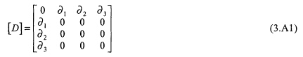
The medium matrix is given by
where k is the compressibility and ρk,r is the volume density of (inertial) mass.
Elastic Waves in Solids
For elastic waves in solids, the spatial differential operator in the system of (3.12) has the following form:
in which
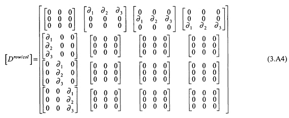
and
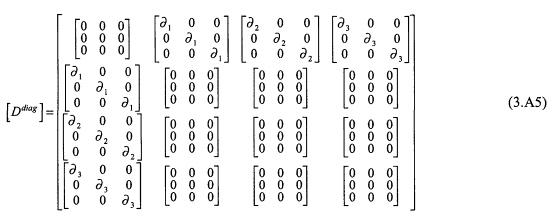
The medium matrix is given by
where ρk,r is the volume density of (inertial) mass and St,j,p,q is the compliance.
Electromagnetic Waves
For electromagnetic waves the spatial differential operator in the system of (3.12) is given by
The medium matrix is found to be
where εk,r is the permittivity and μJ,P is the permeability.


