
Page 89
4
Population Genetics
Much of the controversy about the forensic use of DNA has involved population genetics. In this chapter, we first explain the principles that are generally applicable. We then consider the special problem that arises because the population of the United States includes different population groups and subgroups with different allele frequencies. We develop and illustrate procedures for taking substructure into account in calculating match probabilities. We then show how those procedures can be applied to VNTRs and PCR-based systems. Consider the comparison of DNA from a crime-scene specimen and from a
suspect. (Actually, the evidence DNA need not come from the crime scene, nor the second sample from a suspect, but we use this vocabulary for convenience.) Under current procedures, if the DNA profile from the crime-scene sample reportedly matches that of the suspect, there are two possibilities (aside from error): The DNA at the crime scene came from the suspect or the DNA at the crime scene came from someone else who had the same profile as the suspect. If the DNA profile in question is common in the population, the crime-scene DNA might well have come from someone other than the suspect. If it is rare, the matching of the two DNA profiles is unlikely to be a mere coincidence; the rarer the profile, the less likely it is that the two DNA samples came from different persons.
To assess the probability that DNA from a randomly selected person has the same profile as the evidence DNA, we need to know the frequency of that profile in the population. That frequency is usually determined by comparison with some reference data set. A very small proportion of the trillions of possible profiles are found in any database, so it is necessary to use the frequencies of
Page 90
individual alleles to estimate the frequency of a given profile. That approach necessitates some assumptions about the mating structure of the population, and that is where population genetics comes in.1
Allele and Genotype Proportions
It is conventional in genetics to designate each gene or marker locus with a letter and each allele at that locus with a subscript numeral. So, A10 designates the tenth allele at locus A, B5 the fifth allele at locus B, and so on. When we want a statement to apply to any of the alleles of a given locus, we use a literal subscript, such as i or j. We designate the frequencies (it is customary to use the word frequency for relative frequency, meaning proportion) of alleles with the letter p and a corresponding subscript. Thus, the frequency of allele A3 is p3 and of allele Ai is pi. The sum of all the pi values is 1 because it includes all the possibilities. Symbolically, if S stands for summation, Spi = 1.
At the DQA locus, discussed in Chapter 2, six alleles are customarily used in forensic analysis (Table 4.1). For example, allele D1.1 (designated as 1.1 in the table), has a proportion of 0.150, or 15.0%, in the black population; this was computed from the proportions in the right-hand portion of the table. The first six genotypes include the 1.1 allele (the top one has two copies) and adding their frequencies—0.036 + (0.076 + 0.009 + 0.036 + 0.027 + 0.080)/2—yields 0.150. The division by 2 is because in heterozygotes only half the alleles are D1.1·
Random Mating and Hardy-Weinberg Proportions
In the simplest population structure, mates are chosen at random. Clearly, the population of the United States does not mate at random; a person from Oregon is more likely to mate with another from Oregon than with one from Florida. Furthermore, people often choose mates according to physical and behavioral attributes, such as height and personality. But they do not choose each other according to the markers used for forensic studies, such as VNTRs and STRs. Rather, the proportion of matings between people with two marker genotypes is determined by their frequencies in the mating population. If the allele frequencies in Oregon and Florida are the same as those in the nation as a whole, then the proportions of genotypes in the two states will be the same as those for the United States, even though the population of the whole country clearly does not mate at random.
We use random mating to refer to choice of mates independently of genotype at the relevant loci and independently of ancestry. The expected proportions with
1An elementary exposition of population genetics is found in Hartl and Clark (1989). A more advanced text, with discussion of many of the formulae used here, is Nei (1987). Practical details of estimation and analysis are given by Weir (1990). See also Weir (1995a).
Page 91
| TABLE 4.1 Observed and Expected Frequencies of DQA Genotypes Based on 224 Blacks and 413 Whitesa | |||||
| ALLELES | GENOTYPES | ||||
| Allele Frequency % | Observed (Expected) Frequency % | ||||
| Allele | Black | White | Genotype | Black | White |
| 1.1 | 15.0 | 13.7 | 1.1/1.1 | 3.6(2.3) | 2.2 (1.9) |
| 1.2 | 26.3 | 19.7 | 1.1/1.2 | 7.6 (7.9) | 3.6 (54) |
| 1.3 | 4.5 | 8.5 | 1.1/1.3 | 0.9 (1.4) | 2.9 (2.3) |
| 2 | 12.1 | 10.9 | 1.1/2 | 3.6 (3.6) | 1.9 (3.0) |
| 3 | 11.8 | 20.1 | 1.1/3 | 2.7 (3.5) | 5.3 (5.5) |
| 4 | 30.3 | 27.1 | 1.1/4 | 8.0 (9.1) | 9.2(7.4) |
| 1.2/1.2 | 8.5 (6.9) | 4.6(3.9) | |||
| 1.2/1.3 | 2.2 (2.4) | 3.4 (3.4) | |||
| 1.2/2 | 4.0 (6.4) | 4.6 (4.3) | |||
| 1.2/3 | 7.1 (6.2) | 8.2 (7.9) | |||
| 1.2/4 | 14.7 (16.0) | 10.4 (10.7) | |||
| 1.3/1.3 | 0.0 (0.2) | 1.2 (0.7) | |||
| 1.3/2 | 2.2 (1.1) | 1.5 (1.9) | |||
| 1.3/3 | 1.3 (1.1) | 1.7 (3.4) | |||
| 1.3/4 | 2.2 (2.7) | 5.1 (4.6) | |||
| 2/2 | 2.2 (1.5) | 2.2 (1.2) | |||
| 2/3 | 1.3 (2.9) | 4.8 (4.4) | |||
| 2/4 | 8.5 (7.4) | 4.6 (5.9) | |||
| 3/3 | 0.9 (1.4) | 4.4 (4.0) | |||
| 3/4 | 9.4 (7.2) | 11.4 (10.9) | |||
| 4/4 | 8.9 (9.2) | 6.8 (7.3) | |||
| Homozygotes | 24.1 (21.5) | 21.4 (19.0) | |||
| Heterozygotes | 75.7 (78.9) | 78.6 (81.0) | |||
| aHomozygous genotypes in boldface. Data from Maryland State Crime Laboratory (Helmuth, Fildes, et al. 1990). | |||||
random mating are called the Hardy-Weinberg (HW) proportions, after GH Hardy, a British mathematician, and Wilhelm Weinberg, a German physician. For example, suppose that the proportions of alleles A1, A2, and A3 are p1, P2, and p3, respectively. The proportions of the three alleles among the sperm are given along the top of Table 4.2, and among the eggs, along the left margin. (It is intuitively reasonable and easily demonstrated that random mating is equivalent to combining gametes at random.) The genotypes and their frequencies are given in the interior of the table. The proportion, or frequency, of A1A1 homozygotes is thus p12, and the proportion of A2A3 (we do not distinguish between A2A3 and A3A2) heterozygotes is p2p3 + p3p2 = 2p2p3.
According to Table 4.1, the proportions of alleles D2 and D4 in the white population are 0.109 and 0.271. If we assume HW and treat the sample allele frequencies as if they were the true population frequencies, then the proportion
Page 92
| TABLE 4.2 Hardy-Weinberg Proportions for a Locus with Three Alleles | |||
| Alleles | Alleles (and Frequencies) in Sperm | ||
| A1 (p1) | A2 (p2) | A3 (p3) | |
| A1 (p1) | A1A1 (plpl) | A1A2 (p1p2) | A1A3 (p1p3) |
| A2 (p2) | A2A1 (p2p1) | A2A2 (p2P2) | A2A3 (p2p3) |
| A3 (p3) | A3A1 (p3p1) | A3A2 (p3p2) | A3A3 (p3p3) |
of genotype D2D2 would be (0.109)2 = 0.012, or 1.2%; as Table 4.1 shows, the observed fraction in this sample is 2.2%. The proportion of genotype D2D4 would be 2(0.109)(0.271) = 0.059, or 5.9%; the observed value is 4.6%. Neither of those differences is statistically significant. (Note that genotype D1.3D1.3 was not found in the black database of 224 persons. With multiple alleles and four or five loci, as with VNTRs, most genotypes are not found in any given database.)
The HW relationship is easily stated symbolically. Using letter subscripts for generality, we let pi and pj be the population proportions of two alleles Ai and Aj. If capital letters designate the genotypic proportions, the HW expectations are
![]() (4. 1a)
(4. 1a)![]() (4. 1b)
(4. 1b)
In words, the simple rule is: The proportion of persons with two copies of the same allele is the square of that allele's frequency, and the proportion of persons with two different alleles is twice the product of the two frequencies.
If for some reason a population does not exhibit HW proportions, as will be the case if mating in the previous generation(s) has not been random, only a single generation of random mating is needed to produce HW proportions. This is clear from Table 4.2, which shows that the proportions of gametes that unite to produce individuals in the next generation depend only on the allele frequencies, not the parental genotypes of the current generation. That property adds greatly to the usefulness of Equations 4.1, because it increases the probability that they are accurate. Populations from different parts of the world with different allele frequencies can be homogenized in a single generation, provided that mating is random. Of course, exactly random mating is very unlikely, but the equations are accurate enough for many practical purposes. In Chapter 5 we give estimates of the degree of uncertainty caused by departures from random mating proportions.
Table 4.1 shows how close actual populations come to HW proportions for DQA. The deviations from HW expectations are not great. In the white population, there is a small but statistically significant excess of homozygotes (P » .03);
Page 93
there is an excess in the black population also, but it is not statistically significant.2 It is not unusual to find a slightly higher proportion of homozygotes than predicted. We consider reasons for that later in the chapter.
In forensic applications, we are often interested in the magnitude of a difference, not just its statistical significance.3 In the example above, the deficiency in the observed frequency of heterozygotes is greater in the black population than in the white, but only in the latter is it statistically significant. This is because statistical significance depends strongly on sample size: In large samples, quite small differences can be statistically significant but may not be biologically meaningful.
HW Proportions in a Large Sample
The data in Table 4.1 show approximate agreement with HW expectations, but there is some discrepancy. In the black population, the deficiency of heterozygotes is about 4%, and in the white population, it is about 3%. Most of this discrepancy comes from uncertainty introduced because of the sizes of the databases (224 and 413 persons). With larger samples, we would expect the agreement to be better.
2 The usual x2procedure is weak as a test for departure from HW proportions. The following test has considerably more power to detect departures from equilibrium of particular interest in population genetics (Robertson and Hill 1984). In a database of size N, let Xij denote the number of persons of genotype AiAj. We assume the model
![]()
We want to test the hypothesis that ![]() (i.e., HW proportions; see section on subpopulation theory for a discussion of
(i.e., HW proportions; see section on subpopulation theory for a discussion of ![]() ). It can be shown that a score test, which can be expected to be particularly powerful in detecting small values of
). It can be shown that a score test, which can be expected to be particularly powerful in detecting small values of ![]() , is based on the statistic
, is based on the statistic
![]()
where K is the number of alleles and Qi is the maximum likelihood estimate of pi if ![]() = 0: in this case, Qi is the observed proportion of Ai alleles.
= 0: in this case, Qi is the observed proportion of Ai alleles.
An excess of homozygotes will lead to a positive value of T. Provided that N is large enough, the statistic T has approximately a standard normal distribution if ![]() .
.
In this case, for the white population in Table 4.1, the Xii values are 413(0.022), 413(0.046), . . . : the values of pi are 0.137, 0.197, . . ; N = 413; and K = 6. Substituting those values into the equation gives T = 1.88, which from a table of the normal probability integral gives P » 0.03. For the black population, T = 0.77, giving P » 0.22, where P refers to the probability.
3 The homozygote excess in this data set is larger than is usually found for this locus in more extensive recent studies (such as Rivas et al. 1995). The data in Table 4.1 come from a variety of sources. The data on the black population come mainly from disease-screening programs in California. The data on whites come from a forensic laboratory and from the CEPH (Centre d'Etude du Polymorphisme Humain) collection of family data, stored in France and used for genetic linkage studies.
Page 94
To examine a much larger sample, we consider data on the M-N blood group locus in the New York City white population for six periods between 1931 and 1969. At this locus, there are two alleles, M and N, and therefore three genotypes, MM, MN, and NN. The data include 6,001 persons (12,002 genes). We chose this locus for three reasons. First, there are only two alleles, and all three genotypes are identified. Second, the allele frequencies are close to 1/2, maximizing the power to detect departures from HW ratios. Finally, the observations are highly reliable technically. They are from A. S. Wiener, the leading blood-group expert of the time. New York City is certainly not a homogeneous population. The persistence of two alleles at intermediate frequencies in many populations suggests that these blood groups are subject to natural selection, but the selection is probably weak, and there are only minor allele-frequency differences among various European countries (Mourant et al. 1976, p 251-260).
These blood-group data (Table 4.3) show that, even in a population as heterogeneous as that of New York City, HW ratios are very closely approximated for traits that are not factors in mate selection. The overall heterozygote frequency is within about 1% of its HW expectation. Agreement with HW expectations should be at least as close for loci, such as most of those used in forensics, that are thought to be selectively neutral.
In the United States, bin frequencies within a racial group are usually similar in different regions. The top two graphs in Figure 4.1 show the similar distribution in white populations in Illinois and Georgia. Comparison of the black and the white populations illustrates a point often made by population geneticists—namely, that differences among individuals within a race are much larger than the differences between races. Nevertheless, the intergroup differences are large
| TABLE 4.3 M-N Blood Group Genotypes in New York City Whites a | |||||||
| Sample | Total | MM | MN | NN | PM | PN | Relative Error |
| 1 | 236 | 71 | 116 | 49 | 0.5466 | 0.4534 | 0.0083 |
| 2 | 461 | 132 | 232 | 97 | 0.5380 | 0.4620 | - 0.0123 |
| 3 | 582 | 166 | 289 | 127 | 0.5335 | 0.4665 | 0.0024 |
| 4 | 3,268 | 1,037 | 1,623 | 608 | 0.5656 | 0.4344 | -0.0107 |
| 5 | 954 | 287 | 481 | 186 | 0.5529 | 0.4471 | -0.0198 |
| 6 | 500 | 158 | 249 | 93 | 0.5650 | 0.4350 | -0.0131 |
| Total | 6,001 | 1,851 | 2,990 | 1,160 | 0.5576 | 0.4424 | - 0.0099 |
| aThe columns show the total number, numbers of the three genotypes, the allele frequencies, and the relative error, computed as follows: The expected number of heterozygotes is 2PMPN X Total. For sample I this is 2(0.5466)(0.4534)(236) = 116.975; relative error = (116.975 - 116.0)/1 16.975 = 0.0083, or 0.83%. The sources of the six convenience samples are (1) parents, (2) mothers, (3) patients and hospital staff, (4) donors and paternity cases, (5) professional donors, (6) paternity cases. Data from Mourant et al. (1976), p 274. | |||||||
Page 95
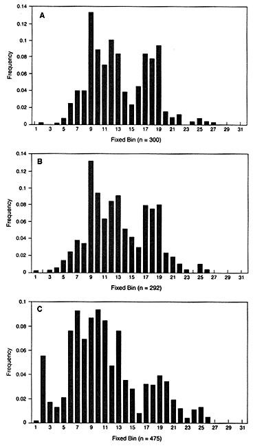
Figure 4.1
Fixed VNTR bins with frequencies of each bin in the United States. The
locus is D2S44 with the enzyme HAE III: (A) Illinois white population, (B)
Georgia white population, (C) US black population. From FBI (1993b),
p 52, 51, 185.
Page 96
enough that the FBI and other forensic laboratories keep separate databases for whites and blacks, and two separate databases for Hispanics, one for those from the eastern United States and another for those from the West.
Exclusion Power of a Locus
The data in Table 4.1 can be used for another purpose. As mentioned in Chapter 2, DQA data can distinguish samples from different individuals 93% of the time, clearing many innocent suspects. The overall probability that two independent persons will have the same DQA genotype is the sum of the squares of the genotype frequencies, as illustrated in Box 4.1.4
| Box 4.1. Calculating the Exclusion Power of a Locus We can illustrate the 93% average exclusion power of DQA by reference to the data in Table 4.1. The probability that two randomly chosen persons have a particular genotype is the square of its frequency in the population. The probability that two randomly chosen persons have the same unspecified genotype is the sum of the squares of the frequencies of all the genotypes. Summing the squares of the expected genotype frequencies (in parentheses) for the black population yields 0.0232 + 0.0792 + . . . + 0.0922 = 0.078. We used expected rather than observed genotype frequencies to obtain greater statistic precision. For the white population, the value is 0.063. The average is about 0.07. The exclusion power is the probability that the two persons do not have the same genotype, or 1 -0.07 = 0.93. If there are n loci, and the sum of squares of the genotype frequencies at locus i is Pi, then the exclusion power is 1-(P1P2. . .Pn). Five loci with the power of DQA would give an exclusion power of 1-(0.07)5 = 0.999998. |
4 The concept of exclusion power was initially described by Fisher (1951). The calculation of the exclusion power can be simplified, especially if the number of alleles is large, by noting that in HW proportions the unconditional probability of identical genotypes is
![]()
Each sum on the right has n terms, where n is the number of alleles, rather than n(n + 1)/2, the number of genotypes. Note that the sum in parentheses on the right-hand side is the homozygosity, fs.
An approximation to the probability of identical genotypes, due to Wong et al. (1987; see also Brenner and Morris 1990), is 2fs2- fs3. This gives the maximum value and is quite accurate for small fs or when the allele frequencies are roughly equal.
Page 97
Table 4.4 shows the frequency of bins (the VNTR equivalent of alleles— See Chapter 2) for two VNTR loci. D2S44 has an exclusion power of about 99%. The exclusion power of D17S79 is smaller because it has fewer alleles and more varied bin frequencies; its exclusion power is about 93%.
Departures from HW Proportions
Clearly, the HW assumption is hardly ever exactly correct. The issue in forensic DNA analysis is whether the departures are large enough to be important. The earlier report (NRC 1992) recommended that databases be tested for agreement with HW expectations and that loci that exhibit statistically significant differences from the expectation be discarded. In our view, that places too much emphasis on formal statistical significance. In practice, statistically significant
| TABLE 4.4 Bin (Allele) Frequencies at Two VNTR Loci (D2S44 and D17S79) in US White Populationa | |||||||
| D2S44 | D17S79 | ||||||
| Bin | Size Range | N | Prop. | Bin | Size Range | N | Prop. |
| 3 | 0- 871 | 8 | 0.005 | 1 | 0- 639 | 16 | 0.010 |
| 4 | 872- 963 | 5 | 0.003 | 2 | 640- 772 | 5 | 0.003 |
| 5 | 964-1,077 | 24 | 0.015 | 3 | 773- 871 | 11 | 0.007 |
| 6 | 1,078-1,196 | 38 | 0.024 | 4 | 872-1.077 | 6 | 0.004 |
| 7 | 1,197-1.352 | 73 | 0.046 | 6 | 1,078-1,196 | 23 | 0.015 |
| 8 | 1,353-1,507 | 55 | 0.035 | 7 | 1,197-1,352 | 348 | 0.224 |
| 9 | 1,508-1,637 | 197 | 0.124 | 8 | 1,353-1,507 | 307 | 0.198 |
| 10 | 1,638-1,788 | 170 | 0.107 | 9 | 1,508-1,637 | 408 | 0.263 |
| 11 | 1,789-1,924 | 131 | 0.083 | 10 | 1,638-1,788 | 309 | 0.199 |
| 12 | 1,925-2,088 | 79 | 0.050 | 11 | 1,789-1,924 | 44 | 0.028 |
| 13 | 2,089-2,351 | 131 | 0.083 | 12 | 1,925-2,088 | 50 | 0.032 |
| 14 | 2,352-2,522 | 60 | 0.038 | 13 | 2,089-2,351 | 16 | 0.010 |
| 15 | 2,523-2,692 | 65 | 0.041 | 14 | 2,352- | 9 | 0.006 |
| 16 | 2,693-2,862 | 63 | 0.040 | 1,552 | 0.999 | ||
| 17 | 2,863-3,033 | 136 | 0.086 | ||||
| 18 | 3,034-3,329 | 141 | 0.089 | ||||
| 19 | 3,330-3,674 | 119 | 0.075 | ||||
| 20 | 3,675-3,979 | 36 | 0.023 | ||||
| 21 | 3,980-4,323 | 27 | 0.017 | ||||
| 22 | 4,324-5,685 | 13 | 0.008 | ||||
| 25 | 5,686- | 13 | 0.008 | ||||
| 1,584 | 1.000 | ||||||
| aD2 and D17 indicate that these are on chromosomes 2 and 17. N is the number of genes (twice the number of persons). Each bin includes a range of sizes (in base pairs) grouped so that no bin has fewer than five genes in the data set; this accounts for nonconsecutive bin numbers. Data from FBI (1993b), p 439, 530; see Budowle, Monson, et al. (1991). | |||||||
Page 98
departures are more likely to be found in large databases because the larger the sample size, the more likely it is that a small (and perhaps unimportant) deviation will be detected; in a small database, even a large departure might not be statistically significant (see Table 4.1 for an example). If the approach recommended in 1992 is followed, the loci with the largest databases, which are the most reliable, would often not be used. As stated earlier, our approach is different. We explicitly assume that departures from HW proportions exist and use a theory that takes them into account. But, as can be seen from the MN data in Table 4.3, we expect the deviations to be small.
Departures from HW proportions in populations can occur for three principal reasons. First, parents might be related, leading to inbreeding. Inbreeding decreases the proportion of heterozygotes, with a compensatory increase in homozygotes.
Second, the population can be subdivided, as in the United States. There are major racial groups (black, Hispanic, American Indian, East Asian, white). Allele frequencies are often sufficiently different between racial groups that it is desirable to have separate databases. Within a race, there is likely to be subdivision. The blending in the melting pot is far from complete, and in the white population, for example, some groups of people reflect to a greater or lesser extent their European origins. A consequence of population subdivision is that mates might have a common origin. Translated into genetic terms, that means that they share some common ancestry—that they are related. Thus, the consequences of population structure are qualitatively the same as those of inbreeding: a decrease of heterozygotes and an increase of homozygotes.5
Third, persons with different genotypes might survive and reproduce at different rates. That is called selection. We shall not consider this possibility, however, because the VNTR and other loci traditionally used in forensic analysis are chosen specifically because they are thought to be selectively neutral or nearly so. Some, such as DQA, are associated with functional loci that are thought to be selected but show no important departures from HW expectations.
Inbreeding and Kinship
Inbreeding means mating of two persons who are more closely related than if they were chosen at random. The theory of inbreeding was worked out 75 years ago by Sewall Wright, who defined the inbreeding coefficient, F (explained in Wright 1951). He gave a simple algorithm for computing F for any degree of
5 There is a theoretical possibility of an increase in heterozygosity. It can happen in a population of first-generation children of different ancestral populations. But such populations are usually mixed with second-generation children, in whom heterozygosity is reduced, and there are other matings. So the effect of population subdivision is to increase homozygosity in the overwhelming majority, if not all, cases.
Page 99
relationship of parents. The kinship coefficient, also designated by F and used to measure degree of relationship between two persons, is the same as the inbreeding coefficient of a (perhaps hypothetical) child.6 For parent and child, F = 1/4; for sibs, 1/4; for half sibs, 1/8; for uncle (or aunt) and nephew (or niece), 1/8; for first cousins, 1/16; and for second cousins, 1/64.
With inbreeding, the expected proportion of heterozygotes is reduced by a fraction F; that of homozygotes is correspondingly increased. Thus, with inbreeding,
![]() (4.2a)
(4.2a)![]() (4.2b)
(4.2b)
Because F for first cousins is 1/16, a population in which everybody had married a first cousin in the previous generation would be 1/16 less heterozygous than if marriages occurred without regard to family relationships.
Population Subgroups
The white population of the United States is a mixture of people of various origins, mostly European. The black and Hispanic populations also have multiple origins. Matings tend to occur between persons who are likely to share some common ancestry and thus to be somewhat related. Therefore, homozygotes are somewhat more common and heterozygotes less common than if mating were random.
The related problem of greatest concern in forensic applications is that profile frequencies are computed (under the assumption of HW proportions) from the population-average allele frequencies. If there is subdivision, that practice will always lead to an underestimate of homozygous genotype frequencies and usually to an overestimate of heterozygote frequencies.
To understand that, consider a population divided into subpopulations, each in HW proportions. Let pi denote the frequency of the allele Ai in the entire population. If that entire population mated at random, the frequencies of the genotypes AiAi and AiAj (i ¹ j) would be pi2 and 2pipj, respectively. The relationship between those hypothetical genotype frequencies and the actual frequencies of homozygotes, Pii, and heterozygotes, Pij, in the entire population is given by
6 Wright's algorithm is given in standard textbooks (Hartl and Clark 1989, p 238ff; see also Wright 1951). One definition of the inbreeding coefficient is the probability that the two homologous genes in a person are descended from the same gene in a common ancestor. The kinship coefficient of two persons is the corresponding probability of identity by descent of two genes, randomly chosen, one from each person. From those definitions, Wright's algorithm can readily be derived. The algorithm is easily modified for genes on the X-chromosome, but since they constitute such a small fraction of the genome, this is an unnecessary refinement for our purposes.
Page 100
Wahlund's principle and its extension to multiple alleles and covariances (Nei 1965). That is,
![]() (4.3a)
(4.3a)![]() (4.3b)
(4.3b)
where Vi designates the variance of the frequency of Ai and Cj the covariance of the frequencies of Ai and Aj among the subpopulations.7
The variance, being the sum of squared quantities, is always positive. The average covariance is negative, because the sum of the variances and covariances over all the alleles must equal zero (because the left-hand terms and first terms on the right, when summed over alleles, must each add to 1). Covariances for specific pairs of alleles, however, might be either positive or negative. In particular, if the allele frequencies are very low and the population is small, they might become positive. If the population is strongly subdivided, the likelihood of positive covariances decreases, because the average value is negative and large.
Thus, to repeat, computing the frequency of a genotype from the population-average allele frequencies, rather than using the average of the actual subpopulation genotype frequencies, will always underestimate the frequency of homozygotes and usually overestimate the frequency of heterozygotes.
As an illustrative example, consider the data in Table 4.5. They come from four white populations—three European and one Canadian. The homozygosities are given in the next-to-bottom line. The weighted average homozygosity for the four populations,8 with weights proportional to the sizes of the databases, is 0.0759. For the pooled populations, assuming that the total pool mated at random, the homozygosity is 0.0745. As the Wahlund principle states, the average homozy-
7Suppose that the proportion of persons in subpopulation k is wk and the frequency of Ai in that subpopulation is p,. Let the random variable pi, denote the frequency of Ai in each subpopulation. Thus. pi = pi,k with probability wk, and the average value of pi is
![]()
Then
![]()
![]()
where
![]()
![]()
8The weighted average homozygosity of the subpopulations, assuming random mating within subpopulations, is Si,k wk pi,k2, where wk is the proportion of persons in the k-th subpopulation and pi,k is the frequency of allele Ai in the k-th subpopulation. The expected homozygosity if the entirepopulation mated at random is Sipi2, where pi = Skwkpi,k·
Page 101
| TABLE 4.5 Bin (Allele) Frequencies and Proportions in Four Populations and Their Weighted Averages a | |||||||||||||
| Canadian | Swiss | French | Spanish | Total | |||||||||
| Bin | ni | pi | ni | pi | ni | pi | ni | pi | n1 | pi | |||
| 1 | 0 | 0.000 | 0 | 0.000 | 0 | 0.000 | 0 | 0.000 | 0 | 0.000 | |||
| 2 | 1 | 0.001 | 0 | 0.000 | 1 | 0.002 | 1 | 0.002 | 3 | 0.001 | |||
| 3 | 1 | 0.001 | 1 | 0.001 | 0 | 0.000 | 3 | 0.005 | 5 | 0.002 | |||
| 4 | 5 | 0.005 | 1 | 0.001 | 3 | 0.005 | 2 | 0.004 | 11 | 0.004 | |||
| 5 | 8 | 0.009 | 13 | 0.016 | 3 | 0.005 | 6 | 0.004 | 30 | 0.011 | |||
| 6 | 21 | 0.023 | 16 | 0.020 | 10 | 0.016 | 7 | 0.014 | 54 | 0.019 | |||
| 7 | 35 | 0.038 | 48 | 0.060 | 26 | 0.042 | 23 | 0.045 | 132 | 0.046 | |||
| 8 | 41 | 0.045 | 30 | 0.037 | 24 | 0.039 | 17 | 0.033 | 112 | 0.039 | |||
| 9 | 130 | 0.142 | 100 | 0.124 | 68 | 0.110 | 52 | 0.102 | 350 | 0.123 | |||
| 10 | 78 | 0.085 | 73 | 0.091 | 67 | 0.109 | 43 | 0.085 | 261 | 0.092 | |||
| 11 | 72 | 0.079 | 67 | 0.083 | 35 | 0.057 | 48 | 0.094 | 222 | 0.078 | |||
| 12 | 81 | 0.088 | 60 | 0.075 | 43 | 0.070 | 24 | 0.047 | 208 | 0.073 | |||
| 13 | 81 | 0.088 | 59 | 0.073 | 56 | 0.091 | 50 | 0.098 | 246 | 0.086 | |||
| 14 | 23 | 0.025 | 24 | 0.030 | 29 | 0.047 | 18 | 0.035 | 94 | 0.033 | |||
| 15 | 19 | 0.021 | 38 | 0.047 | 14 | 0.023 | 19 | 0.037 | 90 | 0.032 | |||
| 16 | 44 | 0.048 | 40 | 0.050 | 27 | 0.044 | 22 | 0.043 | 133 | 0.047 | |||
| 17 | 98 | 0.107 | 71 | 0.088 | 72 | 0.117 | 61 | 0.120 | 302 | 0.106 | |||
| 18 | 69 | 0.075 | 64 | 0.080 | 53 | 0.086 | 36 | 0.071 | 222 | 0.078 | |||
| 19 | 64 | 0.070 | 61 | 0.076 | 48 | 0.078 | 36 | 0.071 | 209 | 0.073 | |||
| 20 | 18 | 0.020 | 12 | 0.015 | 10 | 0.016 | 18 | 0.035 | 58 | 0.020 | |||
| 21 | 11 | 0.012 | 11 | 0.014 | 11 | 0.018 | 13 | 0.026 | 46 | 0.016 | |||
| 22 | 5 | 0.005 | 7 | 0.009 | 8 | 0.013 | 3 | 0.006 | 23 | 0.008 | |||
| 23 | 0 | 0.000 | 2 | 0.002 | 0 | 0.000 | 0 | 0.000 | 2 | 0.001 | |||
| 24 | 1 | 0.001 | 2 | 0.002 | 0 | 0.000 | 3 | 0.006 | 6 | 0.002 | |||
| 25 | 7 | 0.008 | 2 | 0.002 | 5 | 0.008 | 0 | 0.000 | 14 | 0.005 | |||
| 26 | 3 | 0.003 | 2 | 0.002 | 3 | 0.005 | 2 | 0.004 | 10 | 0.004 | |||
| 27 | 0 | 0.000 | 0 | 0.000 | 0 | 0.000 | 0 | 0.000 | 0 | 0.000 | |||
| 28 | 0 | 0.000 | 0 | 0.000 | 0 | 0.000 | 1 | 0.002 | 1 | 0.000 | |||
| Total (2N) | 916 | 0.999 | 804 | 0.998 | 616 | 1.001 | 508 | 0.998 | 2,844 | 0.999 | |||
| Hom. = Spi2 | 0.079 | 0.073 | 0.077 | 0.073 | 0.074 | ||||||||
| fs = 0.0759 | fT= 0.0745 |
| |||||||||||
| aThe bins are numbered (see Table 4.3). The number at the bottom is the total number of genes (twice the number of persons). The locus is D2S44, and the enzyme is Hae III. Data from FBI (1993b), p 461, 464-468. Three French populations were pooled. | |||||||||||||
gosity of the subpopulations is greater and the heterozygosity less than those of the pooled population.
The striking feature of the table is not the greater heterozygosity of the pooled population, which is expected, but the smallness of the difference. The four populations and the composite all differ from HW proportions only very slightly. The data on M-N blood groups (Table 4.3) suggest that this is not surprising.
Page 102
Subpopulation Theory
We can deal with a structured population by using a theory that is very similar to that of inbreeding. We shall reserve the symbol F for inbreeding caused by a specified degree of relationship of the parents, such as cousins. The symbol ![]() is sometimes used in forensic science, so we employ it to designate the effects of population subdivision. The following formulae, which are analogous to those for inbreeding, define a parameter
is sometimes used in forensic science, so we employ it to designate the effects of population subdivision. The following formulae, which are analogous to those for inbreeding, define a parameter ![]() ij for each genotype AiAj. These formulae do not require that the subpopulations mate at random or even that they be distinct.
ij for each genotype AiAj. These formulae do not require that the subpopulations mate at random or even that they be distinct.
![]() (4.4a)
(4.4a)![]() (4.4b)
(4.4b)
In general, the parameters ![]() may be positive or negative. However, substituting the inequalities Pii £ pi and Pij £ 1 into equations 4.4a and 4.4b, respectively, demonstrates that
may be positive or negative. However, substituting the inequalities Pii £ pi and Pij £ 1 into equations 4.4a and 4.4b, respectively, demonstrates that ![]() for every i and j.
for every i and j.
Let f0 denote the actual homozygosity in the entire population, and let h0 = 1 - f0 denote the corresponding heterozygosity. If the population were divided into distinct subpopulations and mating were random within each subpopulation, we would designate fs and hs by fs and hs, respectively. If mating were random within the entire population, these quantities would become fT and hT, respectively.
The average of the parameters ![]() ij over all genotypes is precisely Wright's (1951) fixation index FIT:
ij over all genotypes is precisely Wright's (1951) fixation index FIT:
![]() (4.5)
(4.5)
For an elementary explanation of Equation 4.5 for equal subpopulation numbers, see Hartl and Clark (1989, p 293); Nei (1987, p 162) presents a more detailed treatment. We also provide an alternative and more general derivation (Appendix 4A).
It is clear that ![]() is a composite quantity, averaged over all genotypes, whereas Equations 4.4 involve
is a composite quantity, averaged over all genotypes, whereas Equations 4.4 involve ![]() and
and ![]() for individual genotypes. In general,
for individual genotypes. In general, ![]() may be positive or negative, but
may be positive or negative, but ![]() . However, if the local populations are mating at random or if there is local inbreeding, then the true value of
. However, if the local populations are mating at random or if there is local inbreeding, then the true value of ![]() is positive. In empirical data, if statistical uncertainties are taken into account,
is positive. In empirical data, if statistical uncertainties are taken into account, ![]() is almost always positive or very small. For selectively neutral loci, population values of
is almost always positive or very small. For selectively neutral loci, population values of ![]() for particular genotypes may be negative only temporarily, except in highly unusual situations. Of course, point estimates from samples, which are quite inaccurate, may be negative even when the true value is positive (Weir and Cockerham 1984; Nei 1987; Chakraborty and Danker-Hopfe 1991).
for particular genotypes may be negative only temporarily, except in highly unusual situations. Of course, point estimates from samples, which are quite inaccurate, may be negative even when the true value is positive (Weir and Cockerham 1984; Nei 1987; Chakraborty and Danker-Hopfe 1991).
Most of the forensic literature posits distinct subpopulations in HW proportions. In that case, comparison of Equations 4.4 with Equations 4.3 shows that ![]() ij and
ij and ![]() ij are given by
ij are given by
![]() (4.6a)
(4.6a)
Page 103
![]() (4.6b)
(4.6b)
Because variances are always greater than or equal to zero, we now have ![]() ii ³ 0. However,
ii ³ 0. However, ![]() can be either positive or negative, although its average value is positive, because the average value of the covariance is negative.
can be either positive or negative, although its average value is positive, because the average value of the covariance is negative.
Now ![]() becomes
becomes
![]() (4.7)
(4.7)
which must be nonnegative. The symbols FST (Wright 1951), GST (Nei 1973, 1977), and ![]() (Cockerham 1969, 1973; Weir 1990) have very similar meanings and for our purposes can be regarded as interchangeable (Chakraborty and Danker-Hopfe 1991). According to Equation 4.7, if the subpopulations are distinct and in HW proportions, then
(Cockerham 1969, 1973; Weir 1990) have very similar meanings and for our purposes can be regarded as interchangeable (Chakraborty and Danker-Hopfe 1991). According to Equation 4.7, if the subpopulations are distinct and in HW proportions, then ![]() .
.
Table 4.5 shows that the frequencies in the four populations are quite similar. Furthermore, the values agree well with those from the United States in Table 4.4. The value of ![]() is about 0.0015, as shown in Box 4.2.
is about 0.0015, as shown in Box 4.2.
We chose European populations in the example because they are likely to differ more than the US subpopulations descended from those European countries. The original differences are diminished in the United States by mixing with other groups, so we would expect ![]() calculated for white populations in the United States to be smaller than
calculated for white populations in the United States to be smaller than ![]() calculated for European and Canadian populations.
calculated for European and Canadian populations.
We can use Tables 4.4 and 4.5 for another comparison. Treating the composite European and Canadian populations as one randomly mating subpopulation and the US population as the other, ![]() turns out to be 0.0004. These are, of course. estimates for particular databases, and the estimate is subject to random fluctuation.
turns out to be 0.0004. These are, of course. estimates for particular databases, and the estimate is subject to random fluctuation.
If mating is random in each subpopulation, then ![]() in Equation 4.7 depends only on the allelic (rather than the genotypic) frequencies. In that case,
in Equation 4.7 depends only on the allelic (rather than the genotypic) frequencies. In that case, ![]() can be
can be
| Box 4.2. Calculating From Equation 4.7, we have A glance at Equation 4.7 tells us that |
Page 104
estimated more accurately, because allele frequencies are subject to smaller sampling fluctuations than are genotype frequencies. There are several statistical methods for estimating ![]() from sample allele frequencies. They vary with the assumptions made and the accuracy desired, but the estimates are very close to one another (Weir and Cockerham 1984; Nei 1987; Chakraborty and Danker-Hopfe 1991).
from sample allele frequencies. They vary with the assumptions made and the accuracy desired, but the estimates are very close to one another (Weir and Cockerham 1984; Nei 1987; Chakraborty and Danker-Hopfe 1991).
Taking Population Structure into Account
In the early days of DNA population analysis, there appeared to be a clear excess of homozygotes and a deficiency of heterozygotes (Lander 1989; Cohen 1990). The excess was so large as to suggest a high degree of population stratification; Lander described it as ''spectacular deviations from Hardy-Weinberg equilibrium." The large deviations, however, turned out to be an artifact, a limitation of the laboratory method (Devlin et al. 1990). As discussed in Chapter 2, a single VNTR band does not necessarily indicate a homozygous person. It might arise because a second band is obscured for some reason. When that was taken into account, the excess homozygosity disappeared, and a number of studies have since confirmed that the database populations are very close to HW proportions (e.g., Chakraborty 1991; Chakraborty et al. 1992; Devlin et al. 1992; Risch and Devlin 1992; Weir 1992b,c). It is also illustrated by our numerical examples. Yet, the US population is not exactly in HW proportions. In a large-enough sample, the departure from HW could surely be demonstrated. As emphasized before (NRC 1992), the power of standard methods to detect a statistically significant deviation is very small; very large samples are required. But there are stronger methods that test the level of heterozygosity per se, and we have used one earlier (See Footnote 2).
To restate: Our approach is not to assume HW proportions, but to use procedures that take deviations from HW into account. To do that, we return to discussions of population structure as measured by ![]() .
.
If we assume the population to be subdivided, there are two options. One is to use ![]() empirically. The second is to estimate neither
empirically. The second is to estimate neither ![]() nor the individual values of
nor the individual values of ![]() j, but to take advantage of the fact that for practical purposes they can be assumed to be positive.
j, but to take advantage of the fact that for practical purposes they can be assumed to be positive.
The first option is to measure ![]() empirically and substitute it for
empirically and substitute it for ![]() in Equations 4.4. For US white, black, and Hispanic populations in the FBI databases, the value of
in Equations 4.4. For US white, black, and Hispanic populations in the FBI databases, the value of ![]() is usually less than 0.01—often considerably less (Weir 1994). We illustrated that for D2S44 earlier in this chapter. In particular, the value for whites is estimated (from data obtained from Lifecodes, a commercial DNA laboratory) as 0.002, for blacks 0.007, and for Hispanics 0.009 (Roeder et al. 1995). So deviations of individual subpopulations from HW are likely to be minor.
is usually less than 0.01—often considerably less (Weir 1994). We illustrated that for D2S44 earlier in this chapter. In particular, the value for whites is estimated (from data obtained from Lifecodes, a commercial DNA laboratory) as 0.002, for blacks 0.007, and for Hispanics 0.009 (Roeder et al. 1995). So deviations of individual subpopulations from HW are likely to be minor.
However, for VNTRs we recommend that instead of estimating ![]() ij and applying Equations 4.4, no adjustment be made for heterozygotes and that the
ij and applying Equations 4.4, no adjustment be made for heterozygotes and that the
Page 105
more conservative "2p rule" be used for homozygotes. This rule is explained and justified as follows.
We assume only that ![]() ij is positive for all pairs of alleles. We know that for heterozygotes the HW calculation is generally an overestimate, because from Equation 4.4b the true value includes
ij is positive for all pairs of alleles. We know that for heterozygotes the HW calculation is generally an overestimate, because from Equation 4.4b the true value includes ![]() . The assumption of HW proportions always gives overestimates of heterozygotes when
. The assumption of HW proportions always gives overestimates of heterozygotes when ![]() . Therefore, even if we do not know the actual value of each
. Therefore, even if we do not know the actual value of each ![]() , we can obtain conservative estimates of match probabilities for all heterozygotes by assuming HW proportions. Negative estimates of
, we can obtain conservative estimates of match probabilities for all heterozygotes by assuming HW proportions. Negative estimates of ![]() ij are observed for some data, but these are usually very close to zero and are almost certainly the consequence of sampling errors. In any case, they are usually so small (and thus
ij are observed for some data, but these are usually very close to zero and are almost certainly the consequence of sampling errors. In any case, they are usually so small (and thus ![]() is so close to one) as to have little effect on the calculations.
is so close to one) as to have little effect on the calculations.
That is not the case with homozygotes, as is clear from Equation 4.4a, because with small allele frequencies, a small value of ![]() can introduce a large change in the genotype frequency. However, we can obtain conservative estimates of match probabilities for homozygotes by using the 2p rule. Single bands can be from either homozygotes or heterozygotes in which the second allele has been missed. It has been suggested that a single band at allele Ai be assigned a frequency of 2pi (Budowle, Giusti, et al. 1991; Chakraborty et al. 1992; NRC 1992). That has been criticized for being too conservative because it includes in the frequency estimate several heterozygotes that can usually be ruled out. But an exact correction is not feasible in most cases, because the nature of the missing band is uncertain.
can introduce a large change in the genotype frequency. However, we can obtain conservative estimates of match probabilities for homozygotes by using the 2p rule. Single bands can be from either homozygotes or heterozygotes in which the second allele has been missed. It has been suggested that a single band at allele Ai be assigned a frequency of 2pi (Budowle, Giusti, et al. 1991; Chakraborty et al. 1992; NRC 1992). That has been criticized for being too conservative because it includes in the frequency estimate several heterozygotes that can usually be ruled out. But an exact correction is not feasible in most cases, because the nature of the missing band is uncertain.
We can make a virtue of the suggested procedure. It can be shown9 that if 2pi is assigned to the frequency of a single band at the position of allele Ai, then this simple formula gives an estimate that is necessarily larger than the true frequency. The upper bound always holds, but it is necessary only if some single bands represent heterozygotes. We emphasize that the 2p rule is intended only for loci, such as VNTRs, in which alleles are rare and single bands may be ambiguous.
9 Let X and Y stand for the maternal and paternal alleles at the A locus. A single band at the position of allele Ai can be either an AiAi, homozygote or a heterozygote with one of the alleles being Ai. Thus, we want the probability that at least one allele is Ai:
![]()
For an alternative proof, using standard population genetics methods, note that the probability on the left-hand side of the first equation is equal to
![]()
as above. Clearly, the rule is very conservative because the summation includes a large number of heterozygotes that would be detected as double bands.
Page 106
We arrive at a simple procedure for obtaining a conservative estimate, that is, one that generally underestimates the weight of the evidence against a defendant: Assign the frequency 2pi to each single band and 2pipj to each double band. In arriving at this important conclusion we have made only one assumption: that ![]() is positive. Then the HW rule is conservative, because in a structured population, heterozygote frequencies are overestimated and, with this adjustment, so are homozygote frequencies.
is positive. Then the HW rule is conservative, because in a structured population, heterozygote frequencies are overestimated and, with this adjustment, so are homozygote frequencies.
Empirical data show that with VNTRs departures from HW proportions are small enough for the HW assumption to be sufficiently accurate for forensic purposes. For example, a ![]() -value of 0.01, larger than most estimates, would lead to an error in genotype estimates of about 1%. Nevertheless, to be conservative, we recommend that the HW principle, with the value 2pi, for a single band at allele Ai, be used.
-value of 0.01, larger than most estimates, would lead to an error in genotype estimates of about 1%. Nevertheless, to be conservative, we recommend that the HW principle, with the value 2pi, for a single band at allele Ai, be used.
Multiple Loci and Linkage Equilibrium
With random mating (and in the absence of selection), the population approaches a state in which the frequency of a multilocus genotype is the product of the genotype frequencies at the separate loci. When the population has arrived at such a state, it is said to be in linkage equilibrium (LE). That is a misnomer, in that the principle applies also to loci that are unlinked, as on nonhomologous chromosomes, but we shall adhere to this time-honored convention.
There is, however, an important difference between HW proportions and LE. Whereas, as mentioned earlier, HW proportions are attained in a single generation of random mating, LE is attained only gradually. For pairs of unlinked loci, the departure from LE is halved each generation. Thus, the departure from LE is reduced to 1/2, 1/4, 1/8, . . . of its original value in successive generations. For sets of three or more unlinked loci, the asymptotic rate of approach to LE is still 50% per generation (Nagylaki 1993, p 634 and references therein), so a few generations of random mating bring the population very close to LE, but it does not happen in a single generation.
Loci need not be on nonhomologous chromosomes to attain LE, although loci on the same chromosome approach LE more slowly than those on different chromosomes. For a pair of loci, the departure from LE is reduced to (1-r), (1 -r)2, (l-r)3, . . . of its initial value in successive generations, where r is the rate of recombination between the two loci. For example, DIS80 and D1S7 are both in the same chromosome arm, yet they do not exhibit a statistically significant departure from LE between them (Budowle, Baechtel, et al. 1995). Most forensic applications, however, use loci that are on nonhomologous chromosomes (for which r = 0.5).
The consequence of the gradual approach to equilibrium is that allele combinations that were together in an ancestral population might carry over into contemporary descendants. The mixing process that takes place because of migration
Page 107
and intermarriage generally reduces deviations from linkage equilibrium more slowly than it does deviations from HW proportions.10
Another important difference between HW and LE is that whereas a population broken into subgroups has a systematic bias in favor of homozygosity, departures from LE increase some associations and decrease others in about equal degrees. Although there might be linkage disequilibrium, we would expect some canceling of opposite effects.11 The important point, however, is not the canceling but the small amount of linkage disequilibrium (see below). In this case, multiplying together the frequencies at the several loci will yield roughly the correct answer. An estimated frequency of a composite genotype based on the product of conservative estimates at the several loci is expected to be conservative for the multilocus genotypes.
How Much Departure from LE is Expected?
The main cause of linkage disequilibrium for forensic markers is incomplete mixing of different ancestral populations. We can get an idea of the extent of this in the US white population by asking what would happen in a mixed population derived from two different European countries. There are abundant VNTR data from Switzerland and Spain, so we shall use them for illustration (FBI 1993b).
We shall illustrate this with a particular pair of alleles, one at each of two loci. In each European population, let Pl6 stand for the frequency of bin 16 at locus D10S28, q13 for that of bin 13 at locus D2S44, and P for that of the 16-13 gamete. In each European population, under the assumption of LE, the proportion of gametes with alleles 16 and 13 is p16q13 = P. In the first-generation mixed population, under the assumption of an equal number of migrants from each parent population, the values of p16, q13, and P will be the average of the corresponding parental values, ![]() and
and ![]() . The linkage disequilibrium, the difference between
. The linkage disequilibrium, the difference between ![]() and
and ![]() , is halved each generation, and finally
, is halved each generation, and finally ![]() . Although P changes each generation,
. Although P changes each generation, ![]() does not, since the allele frequencies remain constant. The numerical values are shown in Table 4.6.
does not, since the allele frequencies remain constant. The numerical values are shown in Table 4.6.
The initial linkage disequilibrium is such that P is about 4% greater than its value at LE, but this is reduced to less than 1% by the third generation. These alleles are typical of those in the data set. A more extreme difference is found between bin 25 in D10S38 and Bin 20 in D2S44. In this case, the initial value of ![]() is about 25% less than expected, and the difference is reduced to about 3%
is about 25% less than expected, and the difference is reduced to about 3%
10 With partial mixing, the rate of approach to HW depends on the rate of mixing; for LE. it depends on both the mixing and crossover rates (Nei and Li 1973). For loose linkage, the two rates might be about the same.
11 With two or more loci and linkage, multiple homozygotes might be slightly increased in frequency (Haldane 1949). However, the increase is very slight.
Page 108
| TABLE 4.6 The Approach to LE in a Mixed Populationa | |||||
| pl6 | q13 | p16q13 | P | Difference b | |
| Swiss | 0.030 | 0.073 | 0.00219 | 0.00219 | 0 |
| Spanish | 0.051 | 0.098 | 0.00500 | 0.00500 | 0 |
| Generation |
|
|
|
| Difference |
| 1 | 0.0405 | 0.0855 | 0.00346 | 0.00360 | 0.000140 |
| 2 | . | . | . | 0.00353 | 0.000070 |
| 3 | . | . | . | 0.00350 | 0.000035 |
| 4 | . | . | . | 0.00348 | 0.000018 |
| 5 | . | . | . | 0.00347 | 0.000009 |
| Equilibrium | 0.0405 | 0.0855 | 0.00346 | 0.00346 | 0 |
| aThe population starts with an equal mixture of persons from Spain and Switzerland and mates at random thereafter. The fraction p16 is the frequency of bin 16 at locus D10S28 and q13 is that of bin 13 at locus D2S44. Data from FBI (1993b, p 467, 468, 526, 527). | |||||
| bDifference = P - p16q13· | |||||
by the fourth generation. Four is probably not far from the average number of generations since ancestral migration from Europe.
Many more examples could be chosen, but the general conclusion is that departures from LE are not likely to be large, a few percent at most. The cause of uncertainty in using population averages as a substitute for local data is mainly allele-frequency differences between subpopulations, not departures from HW and LE in each subpopulation.
What Do the VNTR Data Show?
Several authors report agreement with LE or only slight departures from it (Chakraborty and Kidd 1991; Weir 1992a,b, 1993b; Chakraborty 1993). An early study of multiple loci (Risch and Devlin 1992) made use of databases from the FBI and Lifecodes. Risch and Devlin calculated the expected proportion of two-locus matches as the product of the match probabilities at the component loci. From 2,701,834 pairs of profiles in the FBI data involving blacks, whites, eastern Hispanics, and western Hispanics, they calculated an expected total of 95.3 two-locus matches, whereas 104 were observed—not a statistically significant difference.12 Only one three-locus match was found among 7,628,360 pairs of
12 The number 2,701,834 was obtained as follows. In the black database, there were 342 persons in whom alleles at the D1 and D2 loci were recorded; the number of pairs is (342)(341)/2 = 58.31 . There were 350 in whom D1 and D4 were recorded, yielding (350)(349)/2 = 61,075. Continuing through five loci within each of the four groups, the totals are 2,701,834 and 104 two-locus matches, for a rate of 3.8 x 10 5. When persons from different groups were chosen, there were 7,064,26
(footnote continued on next page)
Page 109
profiles; curiously, it was between a white and an eastern Hispanic. There were no four- or five-locus matches (see also Herrin 1993).
If there is no important departure from independence for two loci, it is unlikely that there will be any for larger numbers of loci, but let us nonetheless look at it empirically. To test beyond two loci, it is necessary to use a system in which matches are much more frequent. Lifecodes uses a different enzyme (Pst I) that produces larger fragments, which leads to higher allele frequencies. That made possible a test of three-locus matches in the white population. Whereas 404 were expected, 416 were observed (Risch and Devlin 1992). We conclude that in the large databases of the major races, the populations are quite close to HW and LE.13
That assertion has been questioned by some geneticists. The questions have often not been accompanied by data, but in one exception, a paper that has been frequently quoted in the literature and in court cases, Krane et al. (1992) reported a statistically significant difference in allele frequency between persons of Finnish and Italian ancestry. Subsequent analysis has removed much, but not all, of the discrepancy.14
Geisser and Johnson (1992, 1993) analyzed their data in a way that is different from the usual one, dividing the alleles into quantiles of equal frequency. Their analysis showed statistically significant departures from random proportions. Others fail to find this from comparable data sets (Devlin and Risch 1992; Weir 1993b). The cause of this difference might be the identification of single bands
(footnote continued from previous page)
pairs and 176 matches, for a rate of 2.5 x 10⁻⁵. As expected, the matching frequency is higher within groups, but it is not much higher; the allele frequencies do not differ greatly, even between groups. As has often been emphasized by population geneticists, most of the variability is between persons within groups, not between groups.
13 It has been suggested more than once (e.g., Sullivan 1992) that the FBI sample has been edited and that five-locus matches have been removed. The explanation lies in the inadvertent inclusion of the same person in more than one sample. Almost all such cases were accounted for either by examination of the record or by testing additional loci. Furthermore, the fact that there was only one three-locus match and no four-locus match argues against the reality of any seeming five-locus matches. In a larger study of the TWGDAM database (see below), there were no five-locus matches and only two four-locus matches when six loci were compared. Another example that has been mentioned as evidence of multilocus matches is a highly inbred group, the Karitiana, in the Amazon. See Kidd et al. (1993) for a discussion of the lack of relevance of this example to populations in the United States.
14 Part of the difference lay in simple errors in transcribing data, and another part is attributable to resampling the same persons from small populations (Devlin, Krontiris, et al. 1993). Krane et al. (1992) also emphasized a greater frequency of three-locus matches than that given by the FBI data. But that is to be expected, as it was in the Lifecodes data set; so, although there remains evidence of substructure, the amount is considerably smaller than originally reported. A later study of Finnish and Italian populations showed no such differences (Budowle, Monson, and Giusti 1994), and agreed with data from other populations in various parts of the world (Herrin 1993). But we should note that there are differences among subgroups that would be statistically significant in large samples, but which might be too small to be important.
Page 110
with homozygotes, and we are persuaded by the careful analyses of large data sets by others that the departures are not large enough to invalidate the product rule (with the 2p rule—see below). It has also been argued that there should be a separate database for each region of the United States. The failure to find important departures make that less important than it would have seemed before the large amounts of data were acquired. Unless local variability is much larger than the data indicate, the loss of information from statistical uncertainties in small samples is likely to outweigh any gain from having local databases.
Regardless of whether the population is exactly in LE, the rarity of multilocus matches is evident even in large data bases. As mentioned earlier, Risch and Devlin (1992) found no four- or five-locus matches among 7,628,360 pairs of profiles. The much larger composite database recorded by TWGDAM (Chakraborty, personal communication) comprises 7,201 whites, 4,378 blacks, and 1,243 Hispanics. Among 58 million pairwise comparisons with four, five, or six loci within racial groups, two matches were found for four loci and none for five or six. The matching pairs did not match for the other two loci tested, so this is not a case of DNA from the same person appearing twice in the database. These pairs were necessarily run on different gels, so the precision may have been less than if they had been run on the same gel, and there might have been close relatives in the databases. Nevertheless, the general conclusion is that four-locus matches are extremely rare and five- and six-locus matches have not been seen in these very large databases.
Finally, we can examine conformity to LE in this very large data set accumulated by TWGDAM (Chakraborty, personal communication). The numbers, especially in the white population, are large enough to provide a sensitive test for departure from LE. The data are shown in Table 4.7. The expected number of two- and three-locus matches were calculated from the observed proportion of single-locus matches, assuming LE. As can be seen, when the numbers are large enough for statistical errors to be small, the departures are very small.
| TABLE 4.7 Observed and Expected Numbers of 2-and 3-Locus Matches in the TWGDAM Data Set.a | ||||
| Two Loci | Three Loci | |||
| Expected | Observed | Expected | Observed | |
| White | 33,013 | 33,131 | 321 | 291 |
| Black | 5,137 | 5,246 | 35 | 39 |
| Hispanic | 1,568 | 1,609 | 18 | 25 |
| Indian | 1,964 | 2,320 | 32 | 66 |
| East Asian | 830 | 864 | 6 | 13 |
| aThe calculations were made from data supplied by R. Chakraborty. | ||||
Page 111
The deviation from expected is 0.4% in whites and 2.1% in blacks. These results reinforce the conclusions of Risch and Devlin that VNTR loci are very close to LE. Only in the American Indian population is there an appreciable departure from randomness. That is expected because of the heterogeneous tribal structure.
With LE, we can proceed as follows. If the proportions of alleles Ai and Aj at the A locus are pi and pj and the proportions of Bh and Bk at the B locus are qh and qk, the proportion of the composite genotype AiAj BhBk is (2pipj)(2qhqk) and of AiAj BkBk is(2pipj)(qk2), or (2pipj)(2qk) with the 2p rule, and so on for more than two loci.
Table 4.4 gives examples of VNTR allele (bin) frequencies (Budowle et al. 1991). If A stands for locus D2S44 and B for D17S79 and subscripted bin numbers designate alleles, the probability of genotype A7A11 B7B12 is [2(0.046)(0.083)][2(0.224)(0.032)] = 0.00011, or 1/9,135. If the A locus had a single band at A7, the probability would be calculated conservatively with the 2p rule as [2(0.046)][2(0.224)(0.032)] = 0.00132, or 1/758. It is not surprising that, even with the 2p rule, the calculated probabilities become very small when four or five loci are tested.
Recently, more VNTR loci have been added. The FBI now has a total of seven and some states use eight. If, at each locus, every allele frequency in the profile equaled 0.1 and eight loci were heterozygous, the probability of the profile would be [2(0.1)(0.1)]8 = 2.6 X 10⁻¹⁴, about equal to the reciprocal of 7,700 times the world population. If the population consisted of cousins, with F = 1/16, the probability (see Equation 4.8b) would be 6.6 x 10⁻¹², about the reciprocal of 30 times the world population.
Calculations like those, assuming HW within each locus and LE between loci, illustrate what is called the product rule (NRC 1992). As just stated, when the 2p rule is used for a single band at locus Ai and 2pipj for a double band at alleles Ai and Aj, the calculation is conservative (that is, it generally overestimates the true probability) within loci. Because there is no systematic effect of population structure on the direction of departure from LE and the empirical data show only small departures, we believe it reasonable to regard the product rule with the 2p rule as conservative.
Here is an illustration. Consider the white population frequencies in Table 4.8. Suppose that we have an evidence genotype A6 - B8B14C10C13 D9D16, the dash indicating a single band at allele A6. The calculation is
[2(0.035)][2(0.029)(0.068)][2(0.072)(0.131)][2(0.047)(0.065)] = 3.182 x 10⁻⁸ 1/31 million.
With four or more loci, match probabilities for VNTR loci are usually quite small, as this example illustrates.
How much do racial groups differ? Table 4.8 gives bin frequencies for white, black, and Hispanic populations in the United States for four VNTR loci. Suppose that we have an evidence genotype as above. The probability that a randomly
Page 112
| TABLE 4.8 Bin (Allele) Frequencies of Two VNTR Alleles for Four Loci in Three US Populationsa | ||||
| Locus | Bin | White | Black | Hispanic |
| A. D2S44 | 6 | 0.035 | 0.092 | 0.105 |
| 11 | 0.083 | 0.047 | 0.018 | |
| Number (2N) | 1,584 | 950 | 600 | |
| B. D1S7 | 8 | 0.029 | 0.035 | 0.031 |
| 14 | 0.068 | 0.063 | 0.056 | |
| Number (2N) | 1,190 | 718 | 610 | |
| C. D4S139 | 10 | 0.072 | 0.066 | 0.106 |
| 13 | 0.131 | 0.103 | 0.101 | |
| Number (2N) | 1,188 | 896 | 622 | |
| D. D10S28 | 9 | 0.047 | 0.076 | 0.046 |
| 16 | 0.065 | 0.036 | 0.059 | |
| Number (2N) | 858 | 576 | 460 | |
| a The bins are designated by number (see Table 4.3). N is the number of persons, and 2N is the number of genes in the database. Data from Budowle et al. (1991). The Hispanic sample is from the southeastern United States. | ||||
chosen person from the white population matches this genotype is one in 31 million, in the black population one in 17 million, and in the Hispanic population one in 12 million. The three estimates are within about a factor of 3. Of course, other examples might differ more or less than this one.
We emphasize that, although the product rule with the 2p rule provides a good, if conservative, average estimate, there is uncertainty about individual calculations. That can arise from uncertainties about allele frequencies in the database and from the inappropriateness of the product rule in individual cases. We need some estimate of how far off the calculations in a given case might be. Although small amounts of linkage disequilibrium do not introduce an important systematic bias, they can increase the variability, and therefore the uncertainty, of the estimate. More importantly, however, allele frequencies can differ among subpopulations; although these largely cancel out in the average, the calculations might be inaccurate for a particular person who belongs to a subgroup with frequencies differing from the population average.
Our approach to dealing with such uncertainty is to look at empirical data, as we do in Chapter 5. But, to anticipate the results of the analysis in Chapter 5, the profile frequencies calculated from adequate databases (at least several hundred persons) by our procedures are, we believe, correct within a factor of about 10-fold in either direction.
Page 113
Relatives
It is possible that one or more near-relatives of a suspect are included in the pool of possible perpetrators. That has been discussed by several writers (Lempert 1991, 1993; Evett 1992; Balding and Donnelly 1994a; Balding, Donnelly, and Nichols 1994). The most likely possibility of a relative unknown to the suspect is a paternal half-sibling—a person with the same father and a different mother. Because one or a few relatives in a large population will have only a very slight effect on match probability, we believe that the importance of unknown relatives has been exaggerated. However, there might be other, good reasons to suspect a relative, known or unknown.
If there is evidence against one or more relatives of a suspect, the DNA profiles of such relatives should be obtained whenever feasible. Furthermore. when the pool of possible suspects includes known relatives, determining their profiles might well eliminate them from consideration.
If a suspected relative cannot be profiled, we would want to know the conditional probability that the relative has a particular genotype, given that the suspect is of this type (Weir and Hill 1993). For noninbred unilineal relatives (relatives who have at most one gene identical by descent at a locus), the formulae can be expressed in terms of the kinship coefficient, F. They are as follows:
|
For parent and offspring, F = 1/4; for half-siblings, 1/8; for uncle and nephew, 1/8; for first cousins, 1/16. Other values are easily calculated from Wright's (1951) algorithm.
Full siblings, being bilineal rather than unilineal, require different formulae:
![]() (4.9a)
(4.9a)![]() (4.9b)
(4.9b)
A few other bilineal relatives occur, such as double first cousins, but they are not common. Equations 4.8 and 4.9 depend on the assumption that the population is in HW proportions.
Since VNTR and other forensic loci are unlinked and appear to be close to LE, the conditional probability of a multilocus genotype in a relative is the product of the pertinent single-locus conditional probabilities.
Persons from the Same Subpopulation
In the great majority of cases, very little is known about the person who left the DNA evidence, and the procedures so far discussed are appropriate. It might
Page 114
be known that the DNA came from a white person, in which case the white database is appropriate. If the race is not known or if the population is of racially mixed ancestry, the calculations can be made with each of the appropriate databases and these presented to the court. Alternatively, if a single number is preferred, one might present the calculations for the major racial group that gives the largest probability of a match. Similar procedures can be used for persons of mixed ancestry.
If it is known that the contributor of the evidence DNA and the suspect are from the same subpopulation and there are data for that subpopulation, this is clearly the set of frequencies to use to obtain the most accurate estimate of the genotype frequency in the set of possible perpetrators of the crime. Of course, the database should be large enough to be statistically reliable (at least several hundred persons), and rare alleles should be rebinned (see Chapter 5) so that no allele has a frequency less than five. The product rule is appropriate, in that departures from random mating within a subgroup are not likely to be important (and, as mentioned above, this is supported empirically). The use of the 2p rule makes the product rule conservative.
Some have argued that even if there is no direct evidence, it should be assumed for calculation purposes that the person contributing the evidence and the suspect are from the same subgroup (Balding and Nichols 1994). Even though it is not known to which subpopulation both persons belong, Balding and Nichols assume that the two are likely to be more similar than if they were chosen randomly from the population at large. In our view, that is unnecessarily conservative, and we prefer to make this assumption only when there is good reason to think it appropriate—for example, if the suspect and all the possible perpetrators are from the same small, isolated town. Most of the time, we believe, the subgroup of the suspect is irrelevant.
To continue with the assumption that the person contributing the evidence and the suspect are from the same subgroup, an appropriate procedure is to write the conditional probability of the suspect genotype, given that of the perpetrator. As before, we measure the degree of population subdivision by ![]() , although a single parameter
, although a single parameter ![]() is not sufficient to describe the situation exactly. A number of formulae have been proposed to deal with this (Morton 1992; Crow and Denniston 1993; Balding and Nichols 1994, 1995; Roeder 1994; Weir 1994). They depend on different assumptions and methods of derivation but agree very closely for realistic values of
is not sufficient to describe the situation exactly. A number of formulae have been proposed to deal with this (Morton 1992; Crow and Denniston 1993; Balding and Nichols 1994, 1995; Roeder 1994; Weir 1994). They depend on different assumptions and methods of derivation but agree very closely for realistic values of ![]() and p.15 The simplest of the more accurate formulae is due to Balding and Nichols (1994, 1995):
and p.15 The simplest of the more accurate formulae is due to Balding and Nichols (1994, 1995):
![]() (4.10 a)
(4.10 a)
15 Deriving a formula for these conditional probabilities requires some assumption about the population structure. Some models that have been used are a pure random-drift model, a mutation-drift, infinite-allele model, or a mathematically identical migration-drift infinite-allele model; or
(footnote continued on next page)
Page 115
![]() ( 4.10b)
( 4.10b)
Nothing in population-genetics theory tells us that ![]() should be independent of genotype. In fact, there is likely to be a different
should be independent of genotype. In fact, there is likely to be a different ![]() for each pair of alleles Ai and Aj. Since individual genotypes are usually rare, these values are inaccurately measured and ordinarily unknown. The best procedure is to use a conservative value of
for each pair of alleles Ai and Aj. Since individual genotypes are usually rare, these values are inaccurately measured and ordinarily unknown. The best procedure is to use a conservative value of ![]() in Equations 4.10, knowing that the true individual values are likely to be smaller. Balding and Nichols (1994) extend Equations 4.10 to account for undetected bands. They also give an upper limit for homozygotes, analogous to the 2p rule. Their upper bound on the conditional probability is
in Equations 4.10, knowing that the true individual values are likely to be smaller. Balding and Nichols (1994) extend Equations 4.10 to account for undetected bands. They also give an upper limit for homozygotes, analogous to the 2p rule. Their upper bound on the conditional probability is ![]() . We believe, however, that because Equation 4.10a is already conservative, this rule is usually unnecessary.
. We believe, however, that because Equation 4.10a is already conservative, this rule is usually unnecessary.
The value of ![]() has been estimated for several populations. As mentioned above, typical values for white and black populations are less than 0.01, usually about 0.002. Values for Hispanics are slightly higher, as expected because of the greater heterogeneity of this group, defined as it is mainly by linguistic criteria.
has been estimated for several populations. As mentioned above, typical values for white and black populations are less than 0.01, usually about 0.002. Values for Hispanics are slightly higher, as expected because of the greater heterogeneity of this group, defined as it is mainly by linguistic criteria.
Table 4.9 gives numerical examples of calculations for three racial groups. using the data of Table 4.8. Two alternative assumptions are made: that the evidence profile is heterozygous (there are two clear bands) at all four loci, and that locus A has a single band at allele A6. In this example, the three racial groups are very similar; if all are heterozygous or if the 2p rule is used for homozygotes, they are within a factor of 3. That will not always be true. If one locus is single-banded, the 2p rule makes a substantial difference in the calculation. With four multiallelic loci, such as VNTRs, most four-locus profiles will be heterozygous at all loci. (For example, if the heterozygosity per locus is 0.93, as it is for D2S44, the probability that all four loci will be heterozygous is about 0.75.)
If all loci are heterozygous, then assuming that the evidence DNA and the DNA from the suspect came from the same subpopulation, using Equations 4.10 has a fairly small effect on the calculations when ![]() . However, using a value of
. However, using a value of ![]() decreases the likelihood ratio (increases the match probability—see Chapter 5) by a factor of 10. If the A locus is homozygous, then Equation 4.1 a with the 2p rule is more conservative than Equation 4.10a with
decreases the likelihood ratio (increases the match probability—see Chapter 5) by a factor of 10. If the A locus is homozygous, then Equation 4.1 a with the 2p rule is more conservative than Equation 4.10a with ![]() and very close to Formula 4.10a with
and very close to Formula 4.10a with ![]() .
.
(footnote continued from previous page)
various statistical assumptions concerning the distribution of allele frequencies among the subpopulations. A more appropriate model would be a stepwise-mutation theory because VNTR lengths tend to change by small steps, but that has not been worked out. Even that would not be completely satisfactory unless one also takes migration, which may be more important than mutation, into account. When ![]() is small (< 0.02), the formulae derived from different models agree closely. Although the specific models are highly idealized, when different assumptions lead to similar results, it increases our confidence in the final formulae. The formulae given are from Balding and Nichols (1994), and were chosen because they are both simple to evaluate and accurate.
is small (< 0.02), the formulae derived from different models agree closely. Although the specific models are highly idealized, when different assumptions lead to similar results, it increases our confidence in the final formulae. The formulae given are from Balding and Nichols (1994), and were chosen because they are both simple to evaluate and accurate.
Page 116
| TABLE 4.9 Likelihood Ratio (Reciprocal of Match Probability) for Four-Locus Profiles in Three Populations Calculated by Various Formulaea | |||
| White | Black | Hispanic | |
| Equations 4.1 | |||
| All loci heterozygous | 3.79 x 10⁸ | 3.52 x 10⁸ | 6.56 x 10⁸ |
| A-locus homozygous | 1.80 x 10⁹ | 3.60 x 10⁸ | 2.25 x 10⁸ |
| A-locus single band, 2p rule | 3.14 x 10⁷ | 1.66 x 10⁷ | 1.18 x 10⁷ |
| Equations 4.10, | |||
| All loci heterozygous | 1.20 x 10⁸ | 1.16 x 10⁸ | 1.74 x 10⁸ |
| A-locus homozygous | 2.80 x 10⁸ | 9.87 x 10⁷ | 6.63 x 10⁷ |
| Equations 4.10, | |||
| All loci heterozygous | 2.04 x 10⁷ | 2.06 x 10⁷ | 2.53 x 10⁷ |
| A locus homozygous | 2.48 x 10⁷ | 1.39 x 10⁷ | 1.02 x 10⁷ |
| All Races | |||
| Interim Ceiling Principle | |||
| All loci heterozygous | 2.68 x 10⁶ | ||
| A-locus single-band, 2p rule | 2.68 x 10⁵ | ||
| aThe data are from Table 4.8. The evidence profile is either (1) all loci heterozygous, A6A11 B8B14 C10C13 D9D16, or (2) A-locus single-banded, A6 -. All calculations use the product rule. | |||
For urban populations, 0.01 is a conservative value. A higher value—say, 0.03—could be used for isolated villages.16
The table also gives calculations based on the interim ceiling principle (using 1.645 instead of the value 1.96 cited in NRC 1992—see Chapter 5). As will be explained in Chapter 5, we believe that the ceiling principles are unnecessary. We give the calculation for illustration only.
PCR-Based Systems
As described in Chapter 2, other systems are coming into greater use. Most of them are based on PCR, require much smaller amounts of DNA, and have the additional advantage that the exact allele can usually be determined, so the
16 Empirical estimates of ![]() , essentially the same as FST and GST, are found throughout the population-genetics literature. An extensive compilation is given by Cavalli-Sforza et al. (1994). The values in the compilation are sometimes considerably higher than the values that we use. There are two reasons: The Cavalli-Sforza comparisons are often between major groups, and many of the comparisons are for blood groups and similar polymorphisms, which have much lower mutation rates than VNTRs and are often subject to selection. Selection can differ in different populations; for example, selection for malaria-resistance genes is strong in hot, wet areas. We regard the empirical estimates of
, essentially the same as FST and GST, are found throughout the population-genetics literature. An extensive compilation is given by Cavalli-Sforza et al. (1994). The values in the compilation are sometimes considerably higher than the values that we use. There are two reasons: The Cavalli-Sforza comparisons are often between major groups, and many of the comparisons are for blood groups and similar polymorphisms, which have much lower mutation rates than VNTRs and are often subject to selection. Selection can differ in different populations; for example, selection for malaria-resistance genes is strong in hot, wet areas. We regard the empirical estimates of ![]() from VNTRs, made either from comparison of homozygote and heterozygote frequencies (when the interpretation of single bands is not a substantial problem) or directly by comparisons among groups, as being a much better guide for forensic calculations.
from VNTRs, made either from comparison of homozygote and heterozygote frequencies (when the interpretation of single bands is not a substantial problem) or directly by comparisons among groups, as being a much better guide for forensic calculations.
Page 117
complications of matching and binning are eliminated. That is true for mitochondrial DNA, DQA, and other markers such as STRs.
The newer systems have not had the large amount of population study that VNTRs have had. The databases are smaller, but the studies that have been done show the same agreement with HW and LE that VNTRs do (Herrin et al. 1994; Budowle, Baechtel, et al. 1995; Budowle, Lindsay, et al. 1995). STRs and some of the other loci share the property of VNTRs of not producing a protein product or having any known selectable function. Their chromosomal positions are known, and they can be chosen so that no two are linked. It should be relatively easy to get more population data, because it is not necessary to find the people; DNA samples for large populations already exist.
The previously mentioned advantages of STRs and other new methods (exact genotype determination, fast turnaround, lower cost, and small DNA-sample requirements) are such that the use of these methods will continue to increase. We also expect that population data will continue to accumulate and that tests, particularly of HW and LE, will continue to be carried out; and thus, the new methods will soon be on the same solid footing as VNTRs. Meanwhile, the similarity of some of these loci to VNTR loci and results of studies already done offer evidence that the methods given here will provide to the degree of accuracy required for forensic use.
A locus that is being increasingly used is D1S80. It is also a length variant, but unlike VNTRs, the size of the DNA fragment is small enough to permit PCR analysis. The locus consists of 16-base units, each of which is repeated from 14 to 41 times. It has been validated, both for robustness to environmental insults and for agreement with HW proportions (Sajantila et al. 1992; Budowle, Baechtel, et al. 1995; Cosso and Reynolds 1995).
STR loci appear to be particularly appropriate for forensic use. Like VNTRs, they can be chosen to be in noncoding regions and therefore can be expected to be selectively neutral. Also, they have many alleles, and there are potentially a very large number of loci. Unlike VNTRs, they can be amplified with PCR, and the individual alleles are identifiable.
Table 4.10 compares VNTR loci with two PCR-based systems, STR and Polymarker.17 The total gene diversity is the proportion of heterozygotes that would exist if the entire population were in random-mating proportions. In the table, the gene diversity within subpopulations is given as a fraction of this total
17 The six STR loci represent seven populations from three races, grouped as follows (subgroups within races are in parentheses: east Asians (Chinese, Japanese, Houston Asians), whites (German. Houston), and blacks (Nigeria, Houston). The Polymarker data come from 12 populations from five races: Eskimos (Barrow, Bethel), whites (two US samples, Swiss), blacks (two US samples), Hispanics (three US samples), and east Asians (Chinese, Japanese). Polymarker designations are: DQA (part of the HLA region); LDLR (low density lipoprotein receptor); GYPA (glycophorin A, the MN blood group), HBGG (hemoglobin G gamma globin), D7S8 (a marker of unknown function on chromosome seven), and GC (group specific component).
Page 118
| TABLE 4.10 Comparison of VNTR, STR, and Polymarker Systemsa | |||||||
| Gene Diversity | |||||||
| Proportion | |||||||
| Locus | No. of | Repeat | Total | (a) | (b) | (c) | |
| VNTR loci | £ 31 bins | ||||||
| D1S7 | 9 | 0.9470 | 0.995 | 0.005 | 0.001 | ||
| D2S44 | 31 | 0.9342 | 0.985 | 0.007 | 0.009 | ||
| D4S139 | 32 | 0.9103 | 0.989 | 0.005 | 0.006 | ||
| D10S28 | 33 | 0.9489 | 0.990 | 0.005 | 0.005 | ||
| D17S79 | 38 | 0.8366 | 0.971 | 0.011 | 0.018 | ||
| Mean | 0.9154 | 0.986 | 0.006 | 0.008 | |||
| STR loci | |||||||
| CSFIR | 10 | 4 | 0.751 | 0.987 | 0.005 | 0.008 | |
| THO1 | 8 | 4 | 0.781 | 0.905 | 0.011 | 0.084 | |
| PLA2A | 9 | 3 | 0.814 | 0.945 | 0.004 | 0.051 | |
| F13A1 | 14 | 4 | 0.798 | 0.902 | 0.006 | 0.092 | |
| CYP19 | 10 | 4 | 0.723 | 0.947 | 0.007 | 0.046 | |
| LPL | 7 | 4 | 0.656 | 0.956 | 0.006 | 0.038 | |
| Mean | 0.708 | 0.939 | 0.007 | 0.054 | |||
| Polymarker loci plus DQA | |||||||
| DQA1 | 6 | 0.788 | 0.948 | 0.009 | 0.043 | ||
| LDLR | 2 | 0.483 | 0.914 | 0.004 | 0.082 | ||
| GYPA | 2 | 0.478 | 0.971 | 0.012 | 0.017 | ||
| HBGG | 3 | 0.539 | 0.876 | 0.003 | 0.121 | ||
| D7S8 | 2 | 0.475 | 0.995 | 0.002 | 0.003 | ||
| GC | 3 | 0.654 | 0.909 | 0.003 | 0.088 | ||
| Mean | 0.571 | 0.934 | 0.006 | 0.060 | |||
| a(a) Proportion of gene diversity accounted for by between-individual variability within subpopulations; (b) proportion within races between subpopulations; (c) proportion between races (Chakraborty, Jin, et al. 1995). | |||||||
(a), as are the increments added by subpopulation differences (b) and racial differences (c). As these figures emphasize, for VNTRs, almost all the variability is between individuals within subgroups. Although these proportions, based on limited data sets, suggest that (b) and (c) are approximately the same, in general the divergence between races is larger than that between subgroups within a race (Latter 1980; Chakraborty and Kidd 1991; Devlin and Risch 1992; Devlin, Risch and Roeder 1993, 1994).
The population genetics of the Polymarker loci make these loci less advantageous than VNTRs, for three reasons. First, the number of alleles is small, and that is reflected in the lower gene diversity; several more loci are required than for VNTRs. Second, the variability between races is greater. That is particularly
Page 119
true for the loci LDLR, HBGG, and GC, which are all associated with functional genes (Chapter 2). Third, Polymarker loci have lower mutation rates and are less likely to be selectively neutral than VNTRs and STRs. These factors might cause the differences between groups.
STRs are intermediate in diversity between VNTRs and Polymarkers, as expected given that they have an intermediate number of alleles. The allocation of gene diversity to individual versus group and subgroup differences is also intermediate. Additional data from different STRs in different racial populations are in substantial agreement with the findings presented in the table (e.g., Bever and Creacy 1995; Meyer et al. 1995). An extensive study of blacks, whites, and Hispanics in Houston involving 12 STR loci found a mean heterozygosity (diversity) of about 75%, and 97.6% of the genetic diversity was within racial groups (Edwards et al. 1992; Hammond et al. 1994), in good agreement with the data in Table 4.10.
Compared with VNTRs, STRs have less exclusion power per locus, and Polymarker loci have less than STRs. The power of exclusion depends strongly on the heterozygosity (see footnote 4). Assuming HW proportions and LE and using the data in Table 4.10, the probability that two randomly selected individuals would have the same profile is about 10-10 for the five VNTR loci, about 10-6 for the six STR loci (using the 12 STRs mentioned in the paragraph above would lower the probability to about 10-12), and about 10-4for the six Polymarker loci.
Whereas the total database for VNTRs now numbers in the tens of thousands, the number for the newer systems is still in the hundreds, but the numbers are increasing rapidly, and the studies are being extended to different populations.
It is quite proper to combine different systems (e.g., VNTRs and STRs) in the product rule, provided, of course, that the loci are close to LE.
What do we conclude about PCR-based systems? We believe that they are ready to be used along with VNTRs. Newer data (Chakraborty et al. 1995; Gill and Evett 1995; Promega 1995; Evett, Gill et al. 1996) show low values of ![]() , comparable to those for VNTRs. Within the limitations of the data, there is good agreement with HW and LE. Graphs such as those in Figures 5.3 and 5.4 show about the same degree of uncertainty as VNTRs. Most STRs are at neutral loci. PCR-based systems have fewer alleles and hence higher allele frequencies than VNTRs. This means that the value of
, comparable to those for VNTRs. Within the limitations of the data, there is good agreement with HW and LE. Graphs such as those in Figures 5.3 and 5.4 show about the same degree of uncertainty as VNTRs. Most STRs are at neutral loci. PCR-based systems have fewer alleles and hence higher allele frequencies than VNTRs. This means that the value of ![]() has less influence (see Equation 4.4a). Yet, mutation rates for PCR loci are generally lower than those for VNTRs, and this might lead one to expect greater values of
has less influence (see Equation 4.4a). Yet, mutation rates for PCR loci are generally lower than those for VNTRs, and this might lead one to expect greater values of ![]() .
.
We conclude that PCR-based systems should be used. A value of 0.01 for ![]() would be appropriate. However, in view of the greater uncertainty of PCR-based markers because of less extensive data than for VNTRs, a more conservative value of 0.03 may be chosen.
would be appropriate. However, in view of the greater uncertainty of PCR-based markers because of less extensive data than for VNTRs, a more conservative value of 0.03 may be chosen.
A Conservative Rule for PCR Loci
For VNTRs, we used the 2p rule and showed that it was conservative for populations in which the values of ![]() are positive. The rule was originally
are positive. The rule was originally
Page 120
introduced to adjust for uncertainty as to whether a single band is a homozygote or heterozygote. That problem does not arise with loci at which there is no ambiguity about allele identification. Is there a conservative adjustment for subdivided populations for such loci that corresponds to the 2p rule? It is simple to choose one:18 Assign to each homozygote a frequency pi (rather than pi2). This, however, is unnecessarily conservative.19
A more accurate but still conservative procedure, and one that we recommend, is to use Equation 4.4a with a conservative value of ![]() . Since observed values of
. Since observed values of ![]() are usually less than 0.01, this value would be appropriate. (In view of the greater uncertainty of PCR calculations because of less extensive population data than for VNTRs, a more conservative value of 0.03 might be chosen.) For small, isolated populations, a value of 0.03 is appropriate. This value is intermediate between those that would be found in populations of first- and of second-cousin matings and is a reasonable upper limit for what might be expected.
are usually less than 0.01, this value would be appropriate. (In view of the greater uncertainty of PCR calculations because of less extensive population data than for VNTRs, a more conservative value of 0.03 might be chosen.) For small, isolated populations, a value of 0.03 is appropriate. This value is intermediate between those that would be found in populations of first- and of second-cousin matings and is a reasonable upper limit for what might be expected.
The 2p rule for VNTRs was introduced because single bands may actually come from heterozygotes. If the techniques are or become good enough that this ambiguity does not exist, then VNTRs should be treated like the PCR-based systems, and the procedure of the previous paragraph should be applied. Conversely, even in PCR-based systems, it may be desirable to use the 2p rule if there is uncertainty caused by null alleles. In a well-characterized system, the frequency of null alleles can often be estimated, and a more accurate correction can then be applied.
Development of New Systems
PCR-based systems have several advantages, the most important being that they can be used when source material is sparse or degraded and a second being that there need not be uncertainties of measurement. But there are also
18 Here are two proofs in the style and notation of Footnote 9. First, we have
![]()
Second, note that
![]()
as above.
19 The error involved in assuming HW ratios and ignoring subpopulations makes little difference for heterozygotes. From Equation 4.4b, we see that the frequency is overestimated by a factor ![]() , or approximately
, or approximately ![]() when
when ![]() is small. Furthermore, the error is in the desired direction of conservatism. In contrast, from Equation 4.4a it is seen that the error for homozygotes can be considerable, and in the wrong direction. For example, if pi = 0.03 and
is small. Furthermore, the error is in the desired direction of conservatism. In contrast, from Equation 4.4a it is seen that the error for homozygotes can be considerable, and in the wrong direction. For example, if pi = 0.03 and ![]() , assuming HW gives an estimate of 0.0009. whereas Equation 4.4a gives 0.0018, a two-fold error. But note that this ''p rule" is excessively conservative in assigning a value of 0.03 instead of 0.0018, a 17-fold difference—too conservative, we believe.
, assuming HW gives an estimate of 0.0009. whereas Equation 4.4a gives 0.0018, a two-fold error. But note that this ''p rule" is excessively conservative in assigning a value of 0.03 instead of 0.0018, a 17-fold difference—too conservative, we believe.
Page 121
disadvantages. VNTRs have many alleles, none of which is at a high frequency. Presumably, the high mutation rate accounts for that and for the small differences in frequencies among subgroups.20 The VNTRs used for forensics also occur at loci that have no function and therefore are probably not affected by natural selection. Some of the loci used in PCR-based systems have only a small number of alleles, and the loci are at functional genes, which means that there is less assurance of HW and LE. Many more loci are required to produce the same probability levels than are required for VNTRs.
Yet, the statistical uncertainties with VNTRs (discussed in more detail in Chapter 5) make it desirable to bring new loci into the system. The extensive activity in mapping human genes is leading to the rapid discovery of many more possible markers, some of which are expected to have the kinds of properties that are desirable for forensic use: high mutation rate, multiple alleles, lack of function (which increases the probability of neutrality), speed of analysis, low cost, and unambiguous identification of alleles. We encourage the development and validation of such systems.
Inadequate Databases
There are situations in which the database is inadequate. The population of possible suspects might be so structured that no reasonable average allele frequency can be determined, or there might be no basis for estimating ![]() . Such a situation may be found among some American Indian tribes, Inuits, or isolated immigrant groups. As databases become more extensive and varied, such gaps should be filled.
. Such a situation may be found among some American Indian tribes, Inuits, or isolated immigrant groups. As databases become more extensive and varied, such gaps should be filled.
If an inadequate database is encountered, one procedure is to use allele frequencies from other groups. These should be groups for which the databases are large enough to be reliable, and they should be as closely related to the group in question as possible. We emphasize that they be closely related to discourage the use of a population, possibly unrelated, solely because it has a set of frequencies favorable to the position being argued. For the same reason, we believe that the number of groups examined should be limited. The calculations based on each of the groups, or some sort of average—or if the desire is for the most conservative estimate, the one that is most favorable to the defendant—can be presented to the court.
20 VNTR systems have a high mutation rate, and mutations usually consist of small changes in the length of the VNTR segment. These two factors are largely responsible for the large number of alleles, none of which is very common, in VNTR systems. The resulting high diversity between individuals and small diversity between groups make VNTRs particularly useful as forensic evidence. Although the mutation rates for STRs are not as high as those for VNTRs, the rates are still much higher for STRs than for classical loci. A high mutation rate is desirable for forensic identification (although not for paternity testing).
Page 122
Conclusions and Recommendations
Sufficient data now exist for various groups and subgroups within the United States that analysts should present the best estimates for profile frequencies. For VNTRs, using the 2p rule for single bands and HW for double bands is generally conservative for an individual locus. For multiple loci, departures from LE are not great enough to cause errors comparable to those from uncertainty of allele frequencies estimated from databases.
With appropriate consideration of the data, the principles in this report can be applied to PCR-based systems. For those in which exact genotypes can be determined, the 2p rule should not be used. A conservative estimate is given by using the HW relation for heterozygotes and a conservative value of ![]() in place of
in place of ![]() ii in Equation 4.4a for homozygotes.
ii in Equation 4.4a for homozygotes.
Recommendation 4.1: In general, the calculation of a profile frequency should be made with the product rule. If the race of the person who left the evidence-sample DNA is known, the database for the person's race should be used; if the race is not known, calculations for all racial groups to which possible suspects belong should be made. For systems such as VNTRs, in which a heterozygous locus can be mistaken for a homozygous one, if an upper bound on the genotypic frequency at an apparently homozygous locus (single band) is desired, then twice the allele (bin) frequency, 2p, should be used instead of p2. For systems in which exact genotypes can be determined, ![]() should be used for the frequency at such a locus instead of p2. A conservative value of
should be used for the frequency at such a locus instead of p2. A conservative value of ![]() for the US population is 0.01; for some small, isolated populations, a value of 0.03 may be more appropriate. For both kinds of systems, 2pipj should be used for heterozygotes.
for the US population is 0.01; for some small, isolated populations, a value of 0.03 may be more appropriate. For both kinds of systems, 2pipj should be used for heterozygotes.
A more conservative value of ![]() might be chosen for PCR-based systems in view of the greater uncertainty of calculations for such systems because of less extensive and less varied population data than for VNTRs.
might be chosen for PCR-based systems in view of the greater uncertainty of calculations for such systems because of less extensive and less varied population data than for VNTRs.
Evidence DNA and Suspect from the Same Subgroup
Sometimes there is evidence that the suspect and other possible sources of the sample belong to the same subgroup. That can happen, e.g., if they are all members of an isolated village. In this case, a modification of the procedure is desirable.
Recommendation 4.2: If the particular subpopulation from which the evidence sample came is known, the allele frequencies for the specific subgroup should be used as described in Recommendation 4.1. If allele frequencies for the subgroup are not available, although data for the full population are, then the calculations should use the population-structure Equations 4.10 for each locus, and the resulting values should then be multiplied.
Page 123
Insufficient Data
For some groups—and several American Indian and Inuit tribes are in this category—there are insufficient data to estimate frequencies reliably, and even the overall average might be unreliable. In this case, data from other, related groups provide the best information. The groups chosen should be the most closely related for which adequate databases exist. These might be chosen because of geographical proximity, or a physical anthropologist might be consulted. There should be a limit on the number of such subgroups analyzed to prevent inclusion of more remote groups less relevant to the case.
Recommendation 4.3: If the person who contributed the evidence sample is from a group or tribe for which no adequate database exists, data from several other groups or tribes thought to be closely related to it should be used. The profile frequency should be calculated as described in Recommendation 4.1 for each group or tribe.
Dealing with Relatives
In some instances, there is evidence that one or more relatives of the suspect are possible perpetrators.
Recommendation 4.4: If the possible contributors of the evidence sample include relatives of the suspect, DNA profiles of those relatives should be obtained. If these profiles cannot be obtained, the probability of finding the evidentiary profile in those relatives should be calculated with Formulae 4.8 or 4.9.
Appendix 4A
Here, we derive the relation (Equation 4.5) between the average ![]() of the parameters
of the parameters ![]() and Wright's (1951) fixation index, FIT (Nei 1977, 1987, p 159164; Chakraborty and Danker-Hopfe 1991; Chakraborty 1993). We begin with an arbitrary mating pattern; in particular, we do not assume that random mating occurs within subpopulations, or even that distinct subpopulations occur. Later, we posit distinct subpopulations and random mating in each of them.
and Wright's (1951) fixation index, FIT (Nei 1977, 1987, p 159164; Chakraborty and Danker-Hopfe 1991; Chakraborty 1993). We begin with an arbitrary mating pattern; in particular, we do not assume that random mating occurs within subpopulations, or even that distinct subpopulations occur. Later, we posit distinct subpopulations and random mating in each of them.
The homozygosity, fo, and heterozygosity, h0, in the substructured population are
![]() ,
,
where Pij is the frequency of genotype AiAj. If the entire population mated at random, these quantities would become
![]() ,
,![]()
Page 124
where the allele frequencies pj satisfy
![]()
We can rewrite hT as
![]()
First, we express the homozygote parameters ![]() in terms of the heterozygote parameters
in terms of the heterozygote parameters ![]() . Substituting Equations 4.4 into the equation
. Substituting Equations 4.4 into the equation
![]()
and noting that pi ¹ 0 leads to
![]()
Multiplying that by pi and summing over i enables us to define the mean
![]()
Thus, the weighted means of the homozygote and heterozygote parameters are equal.
We insert Equation 4.4b to deduce that
![]()
If the subpopulations are distinct and mating is random in each subpopulation, then FIT = FST , and hence ![]() .
.


