
Chapter 4
Changes in the Structure of Wages1
BROOKS PIERCE
Texas A&M University
FINIS WELCH
Texas A&M University and Unicon Research
How important is schooling to labor market success? In a word, very. In 1992 white men with a college education earned about 50 percent more per week on average than white men with only a high school education. Fifty percent is a large wage premium to command, yet the premium is even greater if we restrict attention to those relatively young people who completed their schooling in the past 10 years. Furthermore, the difference in labor market opportunities for college versus high school graduates translates into differences in employment, hours worked, industries, and occupations as well as to differences in wages. In 1992 the percentage of college-educated men who worked full time year-round was about 10 points higher than for men with only a high school education, and college-educated men worked on average 200 hours more than men with only a high school education. Those with more schooling were also more likely to find higher-paying white collar jobs. But the variations in these averages are large enough that a college degree is no guarantee of success. For example, in 1992 the probability that a randomly chosen high school graduate earned more than a randomly chosen college-educated worker was over 20 percent. Nevertheless, it is clear that the labor market rewards associated with greater schooling are substantial.
This has not always been the case. In fact, the economic returns to education were much lower only 15 years ago. The rapid divergence in labor market outcomes across schooling groups is only one of the dramatic changes in relative
wages for workers in the United States during the 1980s. In this chapter we summarize what is known about the changing wage structure and some of the more prominent explanations of those changes. The principal findings for the earnings of white men over the past 25 years are that returns to schooling and returns to labor market experience have risen and that wage inequality, both overall and within schooling and experience groups, has risen. The timing and magnitudes of these changes are not always coincident. Inequality increased more or less continually over the same period, but schooling returns actually fell in the 1970s. However, inequality and returns to schooling and experience all rose concurrently in the 1980s. The 1980s were also an interesting period for changing relative wages across gender and racial groups. That period witnessed a pause in the convergence of wages between black and white men as well as the beginnings of rapid wage gains for white women relative to white men.
Validating explanations for these changes has proven difficult, and one would not expect any single factor to account for all of the dimensions of the changing wage structure. However, many of the shifts in relative wages suggest a general rise in the value of what is thought of as generalized ability or "skill." This being the case, researchers have looked to shifts in demand that favor more skilled workers as a possible explanation. Hypotheses about shifts in demand are especially attractive since relative prices and quantities have sometimes moved in the same direction. One possibility is that shifts in product demand—for example, as a result of changing international trade flows—cause some sectors to shrink or grow and result in labor demand shifts in favor of the types of workers employed in the growing sectors. One can assess this theory by determining if expanding industries are the ones that tend to hire more skilled workers. Our impression is that, at least for the education dimension, the data support this version of the demand shift story as a partial explanation. However, most of the change in employment for college graduates is attributable to shifts in industries rather than the changing importance of college-intensive industries.
A second possibility, nonneutral technical change, perhaps linked to the changing availability and power of computers, is often put forward to account for some within-industry employment shifts. This hypothesis is plausible but by its nature difficult to evaluate. One method of accumulating indirect evidence is to determine what types of jobs or occupations are growing. Employment of college-educated workers grew rapidly in the 1970s and 1980s in technical fields such as engineering and computer science and in financial and business-related occupations. In contrast, employment of people with less schooling has shifted toward a different set of occupations, where wages tend to be lower than average. It is not obvious whether this reflects changing labor demand conditions or other factors, such as changing quality of secondary schooling or different raw abilities among those in more recent birth cohorts who do not pursue college degrees. But none of these possibilities suggests that the trends documented below are likely to reverse themselves in the near future.
The Changing Wage Structure
This section summarizes some of the salient features of the changing relative wages over the past 25 years. Our particular concern is with relative wages across different education levels, as most would argue that these groupings indicate real skill differences and that changing relative wages reflect changes in skill returns. To complement the trends in relative prices, we also show trends in relative education quantities. We found that, by and large, relative prices move in favor of higher-skilled workers over the period as a whole. Also, relative quantities are frequently seen to move in the same direction. This suggests that the demand for better-educated workers has risen and perhaps that shifts in labor demand in favor of skilled workers can help rationalize observed changes in other relative wages.
Figure 4.1 presents relative wages between college and high school graduates, measured as a percentage differential among white men. We show series for workers who are one to 10 years out of school and for workers of all experience levels. The series track each other, with more dramatic changes in returns to college for younger workers. Among these younger workers, the wage premium earned by college graduates was about 35 percent in the early years of the data. During the 1970s the premium fell substantially, to a low of about 27 percent in 1979. This drop was likely caused by large increases in the number of people attending college about 1970, either because of the Vietnam War or as part of

FIGURE 4.1 College wage premium by experience level.
rational educational choices by an unusually large birth cohort. The fall was precipitous enough to induce at least one economist to suggest that Americans might be overinvesting in schooling (Freeman, 1976). Yet the fall in returns to a college degree in the 1970s were dwarfed by the rising returns of the 1980s. By the end of the data the college premium was about 55 percent for recent entrants into the job market and 48 percent over all experience levels. It is not much of an exaggeration to say that the college/high school wage premium has doubled in the past 15 years. The similar timing of the two series suggests that this phenomenon reflects something specific to time rather than something specific to birth cohorts. Although in Figure 4.1 the relative earnings of college and high school graduates are plotted rather than each group's earnings levels separately, we show below that the rising college wage premium apparent in the figure is driven largely by declines in the absolute level of real wages of high school graduates. At least as far as the labor market is concerned, the 1990s have been a bad time to be a young high school graduate.
Figure 4.2 shows much the same trends but uses a different metric. Here we plot, for the two different experience groups, the college graduates' average centile location in the earnings distribution for high school graduates. This is the probability that a randomly chosen high school graduate has lower wages than a randomly chosen college graduate. This metric is useful when the relative wage
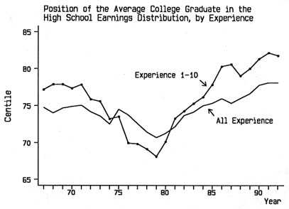
FIGURE 4.2 Relative earnings of college graduates.
dispersion across schooling groups is changing, because it is ordinal in nature.2 For instance, among workers one to 10 years out of school in 1967, the probability that a randomly chosen college graduate had higher earnings than a randomly chosen high school graduate was approximately 77 percent. For this experience group, the probability fell in the early to mid-1970s and then reversed trend and has risen more or less steadily since. Among workers of all experience levels, education returns by this metric follow the same trends but in a more muted fashion. These location statistics seem small given the benchmark of 50 percent for perfect distributional congruence; there is a lot of overlap in the college and high school wage distributions. Also note that the timing and trends in education returns are roughly consistent across the different metrics in Figure 4.1 and 4.2. This implies that the higher college/high school wage ratios of newer entrants in the 1980s reflect ordinal as well as cardinal wage divergence.
One might wonder whether the trends in Figures 4.1 and 4.2 are attributable to some economy-wide changes in the value of the additional skills embodied in a college degree or merely to a change in the quality of newer cohorts of college and high school graduates. One way to address this question is to follow the same cohort of workers as they age. Table 4.1 presents the college/high school wage differential for different cohorts at different points in time. For example, the last number in the first column indicates that among workers who first entered the labor market in 1970 the college/high school wage differential then was 39.2 percent. Moving across columns in the same row indicates what happened to this wage premium as the cohort aged. In the case of the 1970 entry cohort, the college wage premium fell throughout the 1970s, to a low of 27.1 percent in 1980, and then rose fairly rapidly to 36.9 percent in 1985 and 43.2 percent in 1990. The college premiums for other entry cohorts exhibit this same pattern. When following the same cohort of workers, we are holding fixed the quality of the educational instruction and the underlying raw abilities of the different schooling groups at the time they received their education. For the 1970 entry cohort, and the others as well, there is a pattern similar to those in Figures 4.1 and 4.2, and this leads to the suspicion that there is some real change in the value of skills that the college graduates hold. This does not rule out the possibility that the
TABLE 4.1 College Wage Premium by Labor Market Cohort
quality of skills of high school graduates has changed across birth cohorts, but it does indicate that the trends in Figures 4.1 and 4.2 are not solely due to such changes in quality.
To this point the concentration has been exclusively on the college/high school wage premium of white males as a measure of returns to schooling. It is useful, of course, to demonstrate that these trends hold for other demographic groups and at other points in the schooling distribution. Table 4.2 presents the college/high school wage premium for different racial and gender groups. Here we average the premia within subperiods of roughly equal length, with the 1973–1979 period capturing most of the declining schooling returns. Most of these demographic groups have higher college/high school wage premiums at the end of the data than in the 1967–1972 period. In all cases the returns to college graduates rose from the 1973–1979 period to the 1980–1986 period, and in all cases returns rise from 1980–1986 to 1987–1992. The data in Table 4.2 suggest
TABLE 4.2 College Wage Premium by Race and Gender
that the measured phenomenon among white men captures marketwide effects that are also relevant for the other demographic groups.3
Table 4.3 gives measured returns to schooling at various points in the schooling distribution. Here the sample is split into four education groups (0–11, 12, 13–15, and 16 or more years of schooling). Each column gives the average wage earned by those in the stated schooling group relative to the average wage in the next schooling group. As before, wage premiums are given in percentages. These statistics would be fairly sensitive to any changes over time in the underlying raw abilities of the people composing each schooling group, perhaps especially at the lower end of the schooling distribution, and so should be interpreted with care. In most cases, however, the returns to education are greater at the end
TABLE 4.3 Returns to Schooling among White Men, by Schooling Level
of the time period than at the beginning. We take this to mean that trends in the college/high school premium are representative of trends in the returns to schooling more broadly defined.
These changes in relative wages would be expected to affect the amount of time spent working, especially if the wage changes are thought to result largely from shifting relative demand in favor of more skilled workers. Table 4.4 gives various employment measures for the broad schooling groups at different points in time. ''Percent FTYR" gives the percentage by schooling group that worked full time (at least 35 hours per week) and year-round (at least 50 weeks in the year). The columns "Weeks" and "Annual Hours" give the average number of weeks and hours worked per year. All of these measures are positively related to education, although high school graduates and those with some college are similar. These measures have trended downward for all groups but have fallen much more for the lower schooling groups. For example, annual hours worked by college graduates fell by about 25 hours (a little more than 1 percent), as opposed to about 100 hours (about 4 percent) for those with high school or some college education, and about 350 hours (over 15 percent) for those who did not complete high school.
These statistics, plus the fact that average schooling levels have increased substantially in the past 25 years, indicate that the amount of total employment
TABLE 4.4 Employment Status, by Schooling Level, All Experience Levels
attributable to college graduates has risen over time. Table 4.5 gives the changing distribution of employment across the four broad schooling groups. The purpose of the table is to present changes in relative quantities to complement the results given above on changing relative prices. For example, in the period 1967–1972 only about 16 percent of white male workers had a college degree; 20 years later more than 25 percent did. Since the numbers of hours and weeks
TABLE 4.5 Distribution of Workers and Weeks Worked over Schooling Levels, All Experience Levels
worked are lower for the lower schooling groups, and because hours and weeks worked fell much more over time for the lower schooling groups, the distributions of weeks and hours worked show greater shifts toward the college educated. The changes would be even more dramatic if the labor supplied were measured by earnings. The fact that relative quantities shifted toward the higher education groups is important because it adds support to the idea that the changes in returns to schooling over the period as a whole were driven mainly by demand-side phenomena. College-educated workers command a higher wage premium than they once did despite the fact that this group of workers supplies so much more labor now. It is reasonable to interpret much of the observed changes in relative quantities as a supply response to these changing demand conditions.
Industry-Based Composition Effects
The fact that the relative price of college-educated labor increased during a period when its relative quantity rose implies growth in the demand for college graduates that has outpaced any growth in supply. At the same time, other parts of the wage structure have changed in ways consistent with increased demand for skilled workers. Experience returns rose in the 1980s. In addition, the wage premiums enjoyed by males at the top end of the wage distribution rose throughout the 1970s and 1980s. It might be said that the 1980s wage convergence between males and females partly reflected greater returns to cognitive skills, as males disproportionately relied on or worked in jobs that required physical skills.
Identifying the sources of wage structure changes has proven difficult. Given that relative wages and quantities have frequently moved together, some prominent explanations are based on industry-related shifts in demand. For example, changing demands for goods produced domestically, induced by changing trade flows or different income elasticities of demand, could change relative factor demands in favor of those types of workers disproportionately employed in the expanding sectors. Similarly, expansion of certain industries as a result of factor-neutral technical changes could change factor demands. These explanations have some plausibility given the large industrial shifts in the United States in recent years and can, in principle, be verified by analyzing the labor composition of expanding and shrinking sectors. Specifically, with respect to the increased demand for college graduates, growth can be accounted for in one of two ways—either by growth of industries that have greater-than-average demands for college graduates or by individual industries increasing the number of college graduates in the face of a rising relative price for them. The first of these effects entails significant growth in college-intensive industries; the second corresponds to shifts in labor demand in favor of college graduates in individual industries.
To address these possible effects, Table 4.6 shows which industries have expanded and contracted as well as which are college intensive. The first three columns give the share of aggregate workers employed in each of 11 industry
TABLE 4.6 Employment Shares and Percentage College Labor by Industry. 1968–1991
groups in 1968 and 1988 and the percentage change in these shares between those years.4 The final three columns give the fraction of aggregate workers in an industry accounted for by the college educated. 5 The shrinking sectors—agriculture, mining, and the manufacturing industries—tend to be less college intensive than average. For example, 14.6 percent of the employment in durables manufacturing industries during the period 1967 to 1969 was college-educated labor, and
|
4 |
In table 4.6, all quantities refer to fixed-wage weighted aggregates of annual hours across experience, gender, and education cells. For aggregation across education levels, those with less than a high school diploma are assigned a weight of 0.82 for aggregation with high school graduates, and those with 13 to 15 years of schooling are assigned a weight of 0.696 for aggregation with high school graduates and a weight of 0.296 for aggregation with college graduates. Employment shares are calculated as a percentage of the aggregate fixed-wage weighted labor hours employed in the industry. Tables 4.6 and 4.7 present data for three-year windows: 1968 refers to a simple average for the years 1967–1969, and 1988 refers to a simple average for the years 1987–1989. See Murphy and Welch (1993) for further details. |
that sector shrank by 40 percent over the 20-year period. Expanding industries, especially professional and financial ones, tend to be relatively college intensive. In 1968 over 30 percent of the employment in the professional and financial services industry aggregate involved college-educated workers, and employment in that sector grew by about as much as durables manufacturing shrank. The last column in the table also suggests that the within-industry changes in education levels have been extraordinary; the fraction of college labor increased in all industries.
A simple employment change decomposition can help us understand the relative importance of these effects. If the fraction of overall labor employed in industry i in year t is Kit, and the share of college labor in the industry is Rit, the aggregate fraction college, Rt, can be expressed as
and the change in this fraction from year t to year t may be written as
The first term in this expression captures what might be called a "between" effect of changing industrial composition. It is the change in industry share times the difference between the college-educated fraction in the industry and the college-educated fraction in the economy as a whole. If expanding industries are more college intensive than average, this term will be positive. The second term is the "within"-industry effect, measured as a weighted average of changing college intensities, where weights are the fixed industry employment shares. Therefore, changing industry composition cannot contribute to the within-industry effect, which holds industry composition fixed by construction. If explanations based on industry-related demand shifts are correct, the between component of the change in Rt must be substantial and positive. As implemented here, the industry index i ranges over 49 separate industries, the time index t refers to the 1987–1989 period, and the time index t refers to the 1967–1969 period.
Table 4.7 gives results from this decomposition, with the industry classification aggregated up to the industry groups corresponding to Table 4.6. The columns correspond to the between, within, and total effects, respectively. The employment effects listed in column one for particular industries are positive for
TABLE 4.7 Decomposition of Growth in College Employment, 1968–1991
|
Industry |
(1) Between Effect |
(2) Within Effect |
(3) Total Effect |
|
Agriculture and Mining |
0.27 |
0.73 |
1.00 |
|
Construction |
0.00 |
0.67 |
0.67 |
|
Durables Manufacturing |
0.67 |
2.08 |
2.75 |
|
Non-Durables Manufacturing |
0.52 |
1.13 |
1.65 |
|
Transportation and Utilities |
0.04 |
1.30 |
1.34 |
|
Wholesale Trade |
-0.00 |
0.59 |
0.59 |
|
Retail Trade |
-0.17 |
1.86 |
1.69 |
|
Professional and Finance |
1.32 |
2.44 |
3.76 |
|
Education and Welfare |
0.79 |
0.15 |
0.94 |
|
Government |
0.07 |
1.25 |
1.32 |
|
Other Services |
0.24 |
1.06 |
1.30 |
|
All Industries |
3.75 |
13.26 |
17.01 |
|
Notes: Quantities are computed as noted in table 4.1. Columns (1)–(3) give the within- and between-decomposition as described in the text. |
|||
the most part, implying that employment has expanded most in the sectors that hire more college graduates than average and contracted most in the sectors that hire disproportionately more high school graduates. For instance, the contractions in the agriculture/mining and manufacturing industries contributed 1.46 percentage points of the 3.75-percentage-point increase in the share of college labor. Expansions in professional/finance and education/welfare, industries that typically have more educated workers, account for another 2.11-percentage-point increase in the between-industry component.
Although these industry composition changes help explain the increased relative demand for college graduates, they by no means explain the majority of the total effect. The last row of Table 4.7 shows that, for all industries aggregated, 3.75 percentage points of the 17.01-percentage-point increase in the college share of aggregate employment is attributable to the between-industry component. The rest of the growth in college labor over this period is attributable to growth in the college-educated fraction within industries. Since the college-educated fraction of workers increased in each industry group, the within-indus-
try effects in column two are all positive. The demand in growth for better-educated workers in each of these industries was great enough to offset the incentive to substitute away from college labor that is caused by its increased relative cost.6
It is clear from Tables 4.6 and 4.7 that explanations based on industry composition effects can account for only a portion of the demand shift toward college graduates. What, then, can be made of the within-industry changes? One possible explanation is that of a nonfactor-neutral technical change at the level of individual industries. Perhaps a more or less pervasive computer and information revolution has shifted factor demands in favor of better-educated, better-skilled workers. This explanation may strike some as plausible, others as merely a relabeling of our ignorance. In any case, the explanation is difficult to verify or reject given the available data. One approach is to identify the occupations where employment of various education groups rose the most. For instance, do college graduates increasingly go into higher-paying occupations while high school graduates increasingly go into lower-paying ones? Or perhaps there are common themes describing the types of occupations that are growing or shrinking. The next section investigates the possibilities.
Occupational Shifts
The U.S. labor market has become increasingly segmented by schooling levels in the sense that wages and hours-worked differentials have expanded, especially in the 1980s. Some portion of these changes is plausibly related to industry shifts caused by changing product demands. Yet the industrial composition of the U.S. work force does not necessarily reveal much about the tasks performed by workers with different levels of schooling. Examining the occupational composition of various schooling groups gives additional insight into workers' functions.
It would be interesting to know if the schooling-related segmentation observed in wages and employment applies to occupations as well. The types of occupations that high school and college graduates enter and their associated wages also have the potential to reflect any changes in the "quality" of the graduates. For example, what types of jobs do high school graduates typically get? A simple way to approach these issues is to treat the wages of a given schooling group as a weighted average of the wages prevalent in the occupations where that group works. Then, the changing wages of, say, high school graduates can be thought of as deriving from a change in occupations (for given occupational wages) or from a change in the wages of high school graduates in given
occupations holding the occupational distribution fixed. If we let wsot represent average log wages of schooling group s in occupation o at time t, and ƒsot represents the fraction of schooling group s at date t that are in occupation o, the average log wage of schooling group s at date t (wst) is given by
That is, wages are a weighted average (across occupations, with weights given by ƒsot) of occupation-specific wages for that schooling group. Equivalently,
where w*o is the average wage in occupation o that construction does not vary with time or schooling group. The first term captures changes through time in occupational distributions, ƒsot, holding fixed the occupational wage premium w*o. Because this term reflects only movements across occupations, it is a "between-occupation" effect. The second term, however, captures changing wages within occupations (wsot - w*o), and can therefore be thought of as including changing wages "within occupation." This partitioning of wage changes is useful because it separately identifies the component of wage changes due only to changing jobs.
Table 4.8 gives the within/between-occupation schooling premium decomposition for high school and college graduates. Newer entrants (those with one to 10 years of experience) are considered, as well as all experience levels. Two subperiods, 1970–1981 and 1982–1990, must be considered separately because of changes in the occupational classification scheme used in the data. For the purposes of presentation, the wages of each schooling group, and the between-occupation component are normed relative to average wages over each subperiod. For example, the number -5.7 in the first row under "Total" for high school workers indicates that in 1970–1972 young high school workers earned 5.7 percent less than all new entrants in the 1970–1981 subperiod. Of that deficit, 3.3 percentage points can be attributed to high school workers in that time period being in occupations with lower-than-average wages; the remainder of 2.3 percent is attributed to a within-occupation differential. Wages of young high school graduates fell by about 3.1 percent between 1970–1972 and 1979–1981. About four-fifths of the decline can be attributed to a shifting occupational distribution, with young high school graduates increasingly entering occupations with lower-than-average wages. The 1980s saw an even greater erosion in this group's wages, with most but not all of the change attributable to effects within occupational categories.
Compare this to the experience of young college graduates. Wages for this group fell enough in the 1970s that the college/high school wage premium fell during this period (recall Figure 4.1). Most of the decline in the 1970s can be
TABLE 4.8 Between- and Within-Occupation Wage Effects, by Schooling Level
attributed to within-occupation effects. Wages for this group went up slightly in the 1980s, with about one-third of the change attributable to across-occupation shifts and the remainder to a within-occupation phenomenon. The contrast across the college and high school groups in the importance of occupational shifts is interesting; clearly, a portion of the increasing college/high school wage premium between 1970 and 1990 was due to the fact that there was an occupational downgrading among high school graduates. The panel for all experience levels reveals similar patterns—a convergence in the wages of college and high school graduates during the 1970s along with a divergence in the 1980s and a steady erosion in the types of occupations that high school graduates occupy. The college educated experienced no such erosion.
Table 4.9 uses this between/within-occupation methodology to compare the wages of college graduates with those of high school graduates and those with some college (13 to 15 years of schooling). The first four columns compare college graduates and high school graduates. The columns labeled "College Between" and "High School Between" are repeated from Table 4.8, and the columns labeled "Wage Differences" and "Within Differences" are simple differences (across schooling groups) of the ''Total" and "Within" columns, respectively, of Table 4.8. Most of the changing college/high school wage differential can be attributed to within-occupation changes. Yet there is clearly a movement of high school graduates into lower-wage occupations. For example, the wages of these two schooling groups converged by about 3 percentage points during the 1970s for the sample of workers with one to 40 years of experience, even though changing occupational distributions alone indicate a divergence of 2.3 percentage points [(4.3 - 2.3) + (19.2 - 18.9)].
The last four columns of Table 4.9 show the same analysis for the college/some-college comparison. There is not quite as much wage convergence in the 1970s or wage divergence in the 1980s in the college/some-college comparisons, but workers with some college education have typically moved into less lucrative occupations over time. For example, among new workers in the 1970s, the wage premium to college versus some college fell by about 2.1 percentage points (20.6 - 18.5), whereas the movement of the some-college group into lower-paying occupations alone would have resulted in a wage divergence of 5.7 percentage points.
In short, then, the increasing segmentation by schooling level observed in wages and employment does seem to extend to occupations. Table 4.10 identifies the occupations that gained or lost the most employment of given schooling classes along with each occupation's wage premium. 7 For example, in the 1970s the occupational category "Managers, Not Classified Elsewhere" exhibited the
|
7 |
The occupational wage premium is the w*o discussed in the between/within decomposition above, minus the average wage of all workers in this period. The calculations in Table 4.10 are for workers with 1 to 40 years of experience. |
TABLE 4.9 Relative Wage Decompositions
|
|
|
College vs. High School |
College vs. Some College |
||||||
|
|
|
Wage Diff |
College Between |
HS Between |
Within Diff |
Wage Diff |
College Between |
Some Col Between |
Within Diff |
|
A. Experience 1–10 |
|||||||||
|
1970s |
|||||||||
|
|
1970–72 |
36.8 |
19.3 |
-3.3 |
14.1 |
20.6 |
19.3 |
6.8 |
8.1 |
|
|
1973–75 |
32.2 |
18.2 |
-4.0 |
10.0 |
20.9 |
18.2 |
3.9 |
6.7 |
|
|
1976–78 |
27.5 |
15.8 |
-6.1 |
5.7 |
16.0 |
15.8 |
2.8 |
3.0 |
|
|
1979–81 |
30.0 |
17.4 |
-5.9 |
6.6 |
18.5 |
17.4 |
1.1 |
2.2 |
|
1980s |
|||||||||
|
|
1982–84 |
40.6 |
23.3 |
-8.8 |
8.5 |
22.7 |
23.3 |
2.9 |
2.3 |
|
|
1985–87 |
49.1 |
24.8 |
-9.3 |
15.1 |
29.1 |
24.8 |
2.5 |
6.8 |
|
|
1988–90 |
50.0 |
23.8 |
-9.2 |
17.0 |
30.8 |
23.8 |
2.1 |
9.1 |
|
B. Experience 1–40 |
|||||||||
|
1970s |
|||||||||
|
|
1970–72 |
34.2 |
18.9 |
-2.3 |
13.0 |
19.1 |
18.9 |
8.2 |
8.4 |
|
|
1973–75 |
32.1 |
18.9 |
-3.0 |
10.2 |
19.3 |
18.9 |
7.0 |
7.5 |
|
|
1976–78 |
30.9 |
18.0 |
-4.1 |
8.8 |
20.3 |
18.0 |
5.0 |
7.4 |
|
|
1979–81 |
31.2 |
19.2 |
-4.3 |
7.7 |
20.3 |
19.2 |
5.1 |
6.2 |
|
1980s |
|||||||||
|
|
1982–84 |
37.5 |
20.4 |
-7.3 |
9.8 |
25.6 |
20.4 |
3.9 |
9.1 |
|
|
1985–87 |
41.4 |
20.4 |
-8.1 |
12.9 |
26.8 |
20.4 |
3.4 |
9.8 |
|
|
1988–90 |
44.9 |
20.0 |
-8.5 |
16.4 |
28.0 |
20.0 |
2.6 |
10.6 |
|
Notes: Columns labeled "Wage Diff" are wage differentials across the indicated schooling groups, in percentage terms. Columns labeled "Between" are analogous to the "Between'' calculations in table 4.8. Columns labeled "Within Diff" are differences in the "Within" columns of table 4.8 across the relevant schooling groups. See notes to table 4.8 and the text for details. |
|||||||||
greatest absolute increase in employment of college graduates, and workers in that occupation earned wages that were 18.8 percent higher than those of the average worker. The occupation that experienced the greatest decrease in college-educated employment was "dentists," which was associated with an 84.6 percent wage premium during the period examined. Many of the occupations with the largest growth in employment of college graduates in both the 1970s and 1980s are business or finance related. The categories with employment losses are not as clear, although we would note the shrinking elementary and secondary
TABLE 4.10 Occupations with Largest Employment Gains and Losses, by Schooling Level
|
|
Employment Gains |
Employment Losses |
||
|
|
Occupation |
Premium |
Occupation |
Premium |
|
A. College |
||||
|
1970s |
1. Managers, NEC |
18.8 |
Dentists |
84.6 |
|
|
2. Bank Officers/Financial Mgrs. |
34.5 |
Mechanical Engineers |
42.5 |
|
|
3. Physicians |
52.3 |
Sales Engineers |
42.6 |
|
|
4. Accountants |
30.5 |
Sales Representatives, Mfg. |
23.5 |
|
|
5. Sales Representatives, Whse |
14.9 |
Bookkeepers |
-6.9 |
|
1980s |
1. Managers, NEC |
23.3 |
Teachers, Secondary School |
5.4 |
|
|
2. Computer Systems Analysts |
44.8 |
Physicians |
60.9 |
|
|
3. Supervisors, Sales |
-2.4 |
Supervisors, Production |
12.4 |
|
|
4. Other Financial Officers |
35.5 |
Administrators, Education |
30.7 |
|
|
5. Postsecondary Teachers, NEC |
18.8 |
Teachers, Elementary School |
5.0 |
|
B. Some College |
||||
|
1970s |
1. Managers, NEC |
18.8 |
Accountants |
30.5 |
|
|
2. Blue Collar Worker Super. |
8.0 |
Sales Representatives Mfg. |
23.5 |
|
|
3. Truck Drivers |
-14.7 |
Personnel and Labor Relations |
29.4 |
|
|
4. Auto Mechanics |
-17.9 |
Draftsmen |
11.7 |
|
|
5. Restaurant Managers |
-22.2 |
Bank Officers/Financial Mgrs. |
34.5 |
|
1980s |
1. Managers, NEC |
22.3 |
Sales Representatives, Mining |
17.7 |
|
|
2. Correctional Inst. Officer |
-6.7 |
Insurance Sales |
16.9 |
|
|
3. Electricians |
12.7 |
Accountants |
33.7 |
|
|
4. Truck Drivers, Light |
-26.0 |
Supervisors, NEC |
15.1 |
|
|
5. Specified Mechanics |
-10.5 |
Computer Operators |
5.0 |
school occupations in the 1980s. The wage premiums associated with the employment growth occupations in panel A of Table 4.10 are, on average, similar to those of the employment loss occupations.
Panels B through D of Table 4.10 show the same analyses for the other schooling groups. A striking characteristic of these panels is that the occupations with college-educated employment growth have low wages relative to college-educated employment losses. In panel B the workers losing the most labor with 13 to 15 years of schooling are white-collar, high-wage-premium occupations. Large negative wage premiums are especially apparent in the occupations with large employment gains in panels C and D. There is some educational "upgrading" going on within occupations. For example, accountants experienced large
college-educated employment gains but large some-college-educated losses. Similarly, truck drivers experienced large employment gains for high school graduates and large losses for high school dropouts. Although it is difficult to make generalizations based on only a few occupations, the growth in employment for high school graduates in such occupations as "janitors" and "groundskeepers" in the 1980s and the clear movement of those with some college education out of some white-collar and financial services occupations are striking.
There are several possible explanations for the declining occupational placements of workers those with less than 16 years of schooling. One is simply that the economy produces different goods and requires different tasks of its workers
than previously, and workers without the cognitive knowledge-based skills acquired with or implied by a college education can no longer fall back on skilled and semiskilled trades. This is consistent with the shifting industrial composition outlined earlier. An alternative possibility is that the "quality" of high school graduates and those with some college education is not what it used to be. It is likely that with more people going to college the person not continuing beyond high school in 1990 is much different from the person who did not continue beyond high school in 1970. Perhaps even the quality of the instruction received in high school has changed for the worse. Data do not easily permit an evaluation of these possibilities, especially those related to the changing "quality" of high school graduates across different birth cohorts. It is clear that today, for one reason or another, young people without a college education are entering the labor force at an ever-increasing disadvantage.
Summary
Education has become a more important determinant of labor market outcomes in the recent past. This is at least partly the result of economy-wide factors that have acted to increase the demand for relatively skilled workers. It is difficult to imagine that this phenomenon will reverse itself in the immediate future. Indeed, all indications are that it will continue. We are not able to make education policy recommendations based on the broad trends laid out here, but it is clear that now, more than at any time in the past 25 years, improvements in the delivery of education in this country would have large benefits. Increasingly, it appears that secondary-level schooling is successful only insofar as it prepares students for college. The prospects that those who drop out of high school or stop with a high school degree will fare well in the labor market are poor.
References
Freeman, Richard. 1976. The Overeducated American. New York: Academic Press.
Murphy, K. M., and F. Welch. 1992. "The role of international trade in wage differentials." Pp. 101–132. In Workers and Their Wages: Changing Patterns in the United States, Marvin H. Kosters, ed. Washington, D.C.: AEI Press, 1994.
Murphy, K. M., and F. Welch. 1991. "Industrial change and the rising importance of skill." Pp. 39–69. In Uneven Tides: Rising Inequality in America, S. Danziger and P. Gottschalk, eds. New York: Russell Sage Foundation, 1993.


