
Prediction of Unsteady Performance of Marine Propellers with Cavitation Using Surface-Panel Method
Y.-G.Kim (Samsung Heavy Industries Co., Ltd., Korea), C.-S.Lee (Chungnam National University, Korea)
Abstract
This paper describes a low order potential-based panel method formulated for the prediction of the unsteady performance of a cavitating marine propeller that operates behind a ship. The method employs normal dipoles and sources distributed on the blade, hub and wake surfaces to represent the potential flow around the cavitating propeller.
The kinematic boundary condition on the wetted portion of the boundary surface is satisfied by requiring that the normal component of the total velocity should vanish on the boundary surface. By applying Bernoulli's equation, the dynamic boundary condition on the cavity surface is replaced by a kinematic condition; that is, the velocity potential on the cavity surface is expressed in terms of the velocity potential and the perturbation velocity both at the cavity detachment point and other geometric quantities. Sources are introduced to represent the presence of the cavity on the cavitating portion of the body. It is expected that the sources will serve as a normal flux generator, which may be integrated in the streamwise direction to form the cavity shape, in a similar manner as in the thickness problem of the thin wing theory.
The blade and cavity surfaces are discretized into a set of quadrilateral panel elements and the strengths of sources and dipoles are assumed constant at each panel. Applying this approximation to the boundary conditions leads to a set of simultaneous equations. The unsteady problem is treated in discretized time domain by rotating the propeller with constant angular spacing.
In order to reduce computing time and to ensure the convergence, the cavity surface is collapsed to the real blade surface or to the mean wake surface. The linearization in cavity thickness is shown not to deteriorate the accuracy compared to the nonlinear theory.
Systematic numerical tests show that the present numerical method is fast and stable, and is applicable to the 2- or 3-dimensional geometry of arbitrary shape. In order to demonstrate a practical aspect of the present method, sample computations are carried out first for the case of a propeller equipped to a 6300 TEU container ship which has been cavitation-tested behind a full-size model ship, and then for the case of a model propeller operating in screen-generating wake. Comparisons between the predictions and experiments at cavitation tunnels show promising correlation.
1
Introduction
Cavity is known as a major source of noise aboard a ship and fluctuating pressures on the stern hull surface. An ability to predict the behavior of the cavity on propeller blades is therefore in need to design a more comfortable and vibration-free vessel.
When the cavity is absent, the traditional lifting surface method has been applied with success in predicting the global performance of the steady and unsteady performance of marine propellers. See, for example, Kerwin and Lee[1]. The lifting surface approach was then extended to solve the cavitating propeller problem by Lee[2]. The linearized lifting surface theory however shows an unreasonable singular behavior at the leading edge, where the cavity begins. It is therefore expected that the linear theory overpredicts the cavity extent and also the cavity volume, which will consequently lead to overprediction
of the cavity induced pressure impulses on the hull.
Efforts to improve the prediction of the flow around the leading edge followed, among which the work of Kinnas[3] should be noted. He applied the method of Lighthill's correction to the streamwise velocity component obtained in linear theory and was successful in reducing the cavity volume from the original work of Lee[4]. The linear cavity theory is however found later to give a wrong trend by Uhlman[5] and also by Lee et al[6], who show in their nonlinear theory that the predicted cavity extent decreases when the thickness of the blade increases, contrary to the trend in linear theory. The need to treat the finite blade thickness effect is evident.
Recently a surface panel method based on Morino's[7] formulation has been applied successfully to the propeller problem with an improvement on the leading edge solution. Application to the cavitating flow problem is a natural extension. The method was first applied to a two-dimensional hydrofoil problem by Lee[4], Lee et al[6] and also by Kinnas and Fine [8]. They solved the exact nonlinear steady problem, in either partially or super-cavitating steady flow condition.
Kim et al[9] then extended the method for the solution of the 3-D steady and unsteady cavitating hydrofoil problem, where the cavity surface was linearized on the suction side of the blade. By avoiding the linearization in blade thickness as in the lifting surface theory they could maintain the resolution of the flow prediction, especially in the area of the blade leading edge, and hence the cavity behavior could be predicted without loosing accuracy.
The unsteady flow problem around a marine propeller was solved subsequently by Fine[10] and Kim[11]. In the present paper we present the potential-based formulation of Kim[11] to solve the steady or unsteady cavitating propeller flow.
The same formulation is applicable to 2- and 3-dimensional cavity flow problems. To verify the numerical procedure, we first show that the method is applicable to the analysis of the 2-dimensional unsteady hydrofoil in either heave or gust mode for both the partially and super-cavitating flow conditions. We then show the same method is applicable to the 3-dimensional hydrofoil with rectangular plan-form. Finally we predict the cavity behavior around the blades of two marine propeller operating either in screen-generated wake or in wake generated behind a ship model. Our predictions compares fairly well with the cavitation patterns observed at cavitation tunnels.
2
Statement of Boundary-Value Problem
2.1
Basic assumptions
Let's consider a cavitating propeller operating in a nonuniform ship wake with a constant rotational speed n at a constant advance speed Vs. Boundaries such as the rudder and free-surface in contact with the atmosphere are ignored, and the presence of the hull is recognized only by the effective wake, which is assumed to be known. We assume the viscous effect on the blades and the trailing vortex sheets is confined within the infinitesimally thin boundary layer. The cavity is assumed to be a constant pressure surface which grows on the suction side of the blades. We assume that the cavity is a thin sheet cavity and the detachment point of the sheet cavity is known. The ship wake is nonuniform and is assumed undeformable under the influence of the propeller action, and the propeller is operating in an inviscid, incompressible and irrotational fluid field.
2.2
Coordinate systems
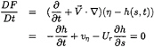
A Cartesian coordinate is chosen as shown in Figure 1; the x-axis coincides with the shaft centerline, defined positive downstream, the positive y-axis points upward, and the z-axis completes a right hand coordinate system. The cylindrical coordinate system is defined for convenience; r being the radius and θ the angle from the positive y-axis positive counter-clockwise when looking downstream.
2.3
Governing equation and boundary conditions
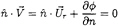
The perturbation velocity ![]() may be expressed by the perturbation velocity potential
may be expressed by the perturbation velocity potential ![]() Then conservation of the mass applied to the potential flow gives the Laplace equation as a governing equation in the fluid region, that is,
Then conservation of the mass applied to the potential flow gives the Laplace equation as a governing equation in the fluid region, that is,
(1)
Motion of the flow satisfying the Laplace equation (1) can be uniquely defined by imposing the following boundary conditions on the boundary surfaces.
-
Kinematic boundary condition(KBC) on the wetted surface

(3)
where
 is the total velocity,
  the unit vector normal to the blade surface, defined positive when pointing into the fluid region.
  is the oncoming flow at a point
  which may be expressed in terms of the effective velocity
  and the rotational velocity
  as follows:
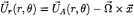
-
Kutta condition at the trailing edge(T.E.):

(4)
-
Kinematic boundary condition(KBC) on the wake surface SW:
(5)
where + and – denote the upper and lower surfaces of the wake, respectively.
-
Dynamic boundary condition(DBC) on the wake surface SW:
Δp=p+–p–=0 (6)
The conditions above are sufficient to describe the fluid motion when the cavity is absent. When the cavity appears, we need additional conditions to be imposed on the cavity surface.
-
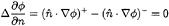
Kinematic boundary condition(KBC) on the cavity surface SC:

(7)
where F(x,y,z,t) is the equation for the cavity surface.
-
Dynamic boundary condition(DBC) on the cavity surface SC:
p=pv (8)
where pv is the vapor pressure inside the cavity.
-
Cavity closure condition:

(9)
where
 represents the cavity thickness function and
  denotes the cavity trailing end position.
3
Integral Equations
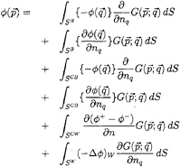
From the Green's theorem, we may derive an expression for the potential in the flow field by distributing the normal dipoles and sources on the body and wake surfaces to deal with the cavity flow problem. The sources on the cavitating portion of boundary surfaces will serve as a normal flux generator, which may be integrated in the streamwise direction to form the cavity shape, in a similar manner as in the thickness problem of the thin wing theory. For brevity, we will not derive the integral equations, but will adopt the final forms only from Kim et al[9].
3.1
Linearization of cavity location
In the nonlinear theory of Lee et al[6], the exact location of the cavity surface is computed iteratively. At each step they relocated the cavity surface where the unknown singularity is distributed and recomputed the induction integrals. Although this procedure could produce the exact solution in the 2-dimensional steady flow, it is obviously impractical for the analysis of the 3-dimensional unsteady cavity flow, due to lack of the robustness of the procedure and unaffordable increase of computing time.
In the present work, the cavity surface is collapsed onto the solid blade surface if the cavity is above the blade surface and onto the mean wake surface if the cavity extends beyond the trailing edge of the blade. The linearization in thickness is not only justified theoretically under the assumption of the thin cavity thickness but also welcomed due to the drastic reduction of the computing time and storage requirements. It is also shown by Kim et al[9] that the linearization does not deteriorate the resolution significantly compared with the nonlinear solution, if a true girth length is considered when evaluating the potential along the cavity surface. Figure 2 shows that the evaluation with the true girth length along the cavity surface(labeled ‘Present Method') compares very well with the nonlinear solution, whereas the evaluation with the girth length of the blade surface(labeled ‘Simply L. M') overpredicts the cavity extent and volume for the case of the partially cavitating flow. This effect is insignificant for the supercavitating flow as shown in Figure 3. This will be illustrated further later.
3.2
Fully wetted flow or partially cavitating flow
The perturbation velocity potential is expressed as follows:
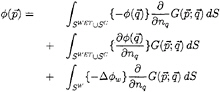
(10)
where ![]() is the Green's function, and
is the Green's function, and ![]() the control and singularity points, respectively. SB, SC and SW represent the body, cavity and wake surfaces, respectively.
the control and singularity points, respectively. SB, SC and SW represent the body, cavity and wake surfaces, respectively.
3.3
Supercavitating flow
The perturbation velocity potential is expressed as follows:
(11)
where SWET denotes the wetted surface, and SCB and SCW denote the supercavitating portion projected upon the blade surface and wake sheet, respectively. The superscripts + and – denote both sides of the cavity extending beyond the trailing edge with the positive sign for the surface connecting the suction side of the blade.
Due to the characteristics of singularities, the governing equation (1) and the quiescence condition (2) will automatically be satisfied.
We know the strength of the sources distributed on the wetted portion of blades from (3) and that of normal dipoles on the cavity from (8) (as will be described later), and hence (10) and (11) become integral equations for the unknown strengths of the sources on the cavity surface and the normal dipoles on the wetted surface.
4
Numerical Implementation
4.1
Discretization of propeller blades and wake
For numerical computation, the propeller and cavity surfaces are replaced by a set of non-planar quadrilateral panels as shown in Figure 4. The flow near the leading edge and tip of the blades varies more rapidly than any other region around the blade, and hence the surface panel size should be smaller in this region. We adopted a so-called cosine spacing in the chordwise direction and a half-cosine spacing in the radial direction, as is evidenced in Figure 4.
Modeling of the shed vortex wake is very important in accurately predicting the performance. We adopted the Greeley and Kerwin's nonlinear wake model which is derived from the LDV measurement at the cavitation tunnel. Figure 5 shows the wake panels trailing a single blade. Details for discretization of the blade and shed wake may be found in Kim [11].
4.2
Numerical procedure
After discretization, we assume the singularity strength be constant on each panel, and then the integral equations (10) and (11) can be replaced into a set of simultaneous equations with unknown strengths of the potential or the normal derivative of the potential. With a proper use of the cavity KBC (7) and the closure condition (9), we may also determine the cavity shape and the cavity volume.
For the unsteady behavior, we solve the boundary-value problem iteratively by advancing the propeller by a discrete angular spacing in time domain as in Lee[2]. The cavity extent is a part of the solution, which has to be known in advance to distribute appropriate singularities on the panel surfaces. We therefore have to resort to another iterative procedure for search of the cavity extent; that is, one in the chordwise direction and the other in the spanwise direction. As is proved in Lee[2], this space-domain iteration is found very efficient and shows very fast convergence characteristics.
Besides the Green functions, the only significant difference between 2-dimensional and 3-dimensional problems in the present numerical procedure is the interaction between the chordwise strips. Once adopted the spanwise iterative procedure we may confine the analysis onto the only one chordwise strip with the influence of the other strips assumed known or updated through iteration. In the subsequent sections, we will restrict the formulation along
a particular chordwise strip without mentioning the influence of the other strip and also that of the other blades. The hub is present in all sample computations, but will not be included in the formulation for brevity.
4.3
Unsteady DBC on cavity surface, SC
If we apply Bernoulli's equation to the cavity surface SC, we have
(12)
where ![]() and Ys denotes the vertical coordinate in ship-fixed coordinate system, g the gravitational acceleration.
and Ys denotes the vertical coordinate in ship-fixed coordinate system, g the gravitational acceleration.
We define the cavitation numbers σn and σ as follows:
(13)
where Js denotes the advance coefficient based on the ship speed.
Since the DBC has to be satisfied along the cavity surface, we have
(14)
where R denotes the propeller tip radius.
Let us define the Froude number as follows:
(15)
Then (14) may be expressed as follows:
(16)
If we apply (16) on an arbitrary point with index j and the cavity detachment point (cdp) at the blade leading edge, we obtain the following: (For convenience, all physical variables are to be nondimensionalized; that is, the speed by Vs, the length by R and the velocity potential by RVs. We will use the same symbols after nondimensionalization.)
(17)
where the subscript c denotes a point on the cavity surface.
Keeping in mind the iteration scheme, (17) may be rearranged as follows:
(18)
where the superscript * denotes that the corresponding variable is assumed known from the previous time step or updated through iteration.
Noticing that the perturbation tangential speed vc on SC is always larger than the tangential speed of oncoming flow, we may express the perturbation speed on SC as follows:
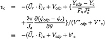
(19)
where ![]() denotes the unit tangential vector along the chordwise direction.
denotes the unit tangential vector along the chordwise direction.
4.4
Discretization of DBC on cavity surface, SC
Using (19) derived from the dynamic boundary condition on the cavity surface, we may express the velocity potential on the cavity as follows:
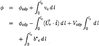
(20)
where lg denotes the girth length along the cavity surface from the cavity detachment point to the point where the potential is calculated.
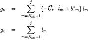
The perturbation potential at the j-th control point on the chordwise strip may now be expressed in discretized form as follows:
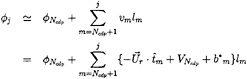
(21)
where Ncdp denotes the panel index of the cavity detachment point. In (21), note that the dummy index m are defined around the blade section beginning from 1 at the lower surface of the trailing edge leading to NP at the upper surface of the trailing edge.
The speed at the cavity detachment point ![]() is the only unknown quantity within the braces in (21), since all the other quantities are already known or may be evaluated from the previous time step. The perturbation potential on the cavity surface may now be recast as follows:
is the only unknown quantity within the braces in (21), since all the other quantities are already known or may be evaluated from the previous time step. The perturbation potential on the cavity surface may now be recast as follows:
(22)
where
(23)
4.5
Influence of dipoles and sources on cavity surface, SC
We assume that the strengths of potential and its normal derivative are constant on each panel, and thus in all subsequent analysis, the induction integrals are to be separated out and be evaluated analytically.
The potential induced by dipoles on SC may be expressed, using (22), as follows:
(24)
Note that there are only two unknowns, ![]() and
and ![]() in the above equation.
in the above equation.
The potential induced by the sources, ∂![]() /∂n, on the cavity surface, SC, may also be discretized as:
/∂n, on the cavity surface, SC, may also be discretized as:
(25)
where NC denotes the number of cavity source panels in the chordwise strip in question and ![]() the quadrilateral element where the integration will be performed.
the quadrilateral element where the integration will be performed.
4.6
Numerical Kutta condition
Kutta condition (4) should be implemented appropriately depending upon the formulation. In the present study, we follow the form derived by Kim[11] as follows:
{∆![]() }T.E.=
}T.E.=![]() NP–
NP–![]() 1+H (26)
1+H (26)
where the function H is defined as a function of the geometrical quantities at the trailing edge and the potential variation at the panel adjacent the trailing edge. We observe that the first two terms in (26) are the terms found in the Morino's numerical Kutta condition[7]. Kim[11] showed that the last term H is negligible near the mid-radius but becomes significant in the blade tip region.
4.7
Influence of shed dipoles on trailing wake, SW
The strength and the position of the trailing dipoles in wake should be determined in principle by satisfying the kinematic and dynamic boundary conditions on the wake surface. In linear theory, the trailing vortices shed downstream with the speed of the oncoming uniform flow, while keeping the strength obtained when leaving the trailing edge of the blade. The strength of the dipole at time t, in θW may be expressed by the potential jump at the trailing edge as follows:
(27)
From (27) the potential induced by the shed dipole is expressed as follows:
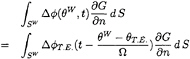
(28)
Equation (28) may be discretized as follows:
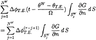
(29)
where τ and j denote the present time step and the dipole index located in shed wake, respectively.
4.8
Discretization of integral equation for partially cavitating flow
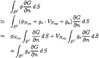
Applying (10) to the i-th control point either on ![]() or on SC, we obtain the following equation, that is,
or on SC, we obtain the following equation, that is,
(30)
where NWET and NW denote the number of cavity panels on the wetted portion of the blade and that in the wake, respectively.
The normal flux ∂![]() /∂n is known on the wetted portion of the blade
/∂n is known on the wetted portion of the blade ![]() by the kinematic boundary condition (3), while it remains to be unknown on the cavitating portion SC, and hence (30) may be rearranged as:
by the kinematic boundary condition (3), while it remains to be unknown on the cavitating portion SC, and hence (30) may be rearranged as:
(31)
As observed in (24), the potential on SC or the second term in (31) may be replaced by terms containing ![]() and other known quantities. Applying at the same time the numerical Kutta condition(26) and also rearranging all known terms in the right hand side, we obtain for the i-th control point the final form for the partially cavitating flow as follows:
and other known quantities. Applying at the same time the numerical Kutta condition(26) and also rearranging all known terms in the right hand side, we obtain for the i-th control point the final form for the partially cavitating flow as follows:
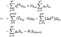
(32)
where
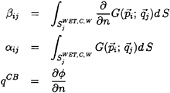
(33)
The influence functions above have to be evaluated on the appropriate quadrilateral elemental areas as indicated by the superscripts. Note that for the self-induced potential of the dipole βii=0.5. We introduce a new symbol qCB to represent the cavity source above the blade surface.
4.9
Discretization of integral equation for supercavitating flow
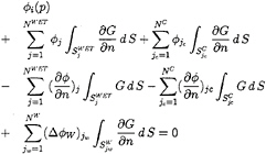
Applying (11) to the i-th control point on SC, we obtain the following equation for the supercavitating flow, that is,
(34)
where NCB and NCW are the number of panels on SCB and SCW, respectively, giving NC=NCB+ NCW, and the cavity sources in the wake is represented as:
(35)
Rearranging (34) we obtain
(36)
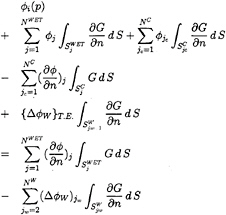
The equation (36) takes a different form depending upon the position of the control point as give below. Again we apply the relation (22) to express the potential on the cavity surface.
When the control point falls on ![]() or SCB, (36) becomes as follows:
or SCB, (36) becomes as follows:
(37)
For the Kutta condition in supercavitating flow, we use the relation (26) without H term. For the potential on the upper surface of the trailing edge, we used from (22) the relation ![]()
When the ic-th control point falls on SCW, recalling that the potential at the control point on the cavity is ![]() from (22), we obtain the following:
from (22), we obtain the following:
(38)
4.10
Cavity closure condition and representation of cavity shape
The cavity closure condition (9) assumes that the thickness of the cavity along its boundary surface outline should vanish. To derive a relation between the cavity shape and the source strengths on the cavity, we take time derivative to the cavity surface function F=η–h(s,t)=0 along the surface and linearize on the cavity surface to obtain (neglecting the spanwise derivative)
(39)
In the present linearized problem, the real cavity surface is collapsed upon the upper surface of the blade. We will satisfy the dynamic boundary condition only on the cavitated portion of the blade to determine the strength of the normal flux ∂![]() /∂n, This term may be considered an error in kinematic boundary condition on linearized cavity surface and be related to cavity thickness as follows:
/∂n, This term may be considered an error in kinematic boundary condition on linearized cavity surface and be related to cavity thickness as follows:
(40)
The cavity thickness, Tc(s,t) may be defined as the difference of the upper and lower surfaces of the cavity h+(s,t) and h–(s,t). In the present partially cavitating flow, the lower surface coincides with the blade surface. Equation (40) is a one-dimensional wave equation and has to be solved in time and space.
Since we assume the unsteadiness is small in the present study, we drop without proof the time derivative term to simplify our numerical procedure.
As in thin wing theory, the cavity thickness function is then expressed as an integral of the normal flux obtained in (40)
(41)
The cavity closure condition requires that the thickness at the cavity trailing end(cte) be zero, that is, Tc(scte,t)=0, and hence we have
(42)
We may discretize the above equation and rearrange to obtain, recalling (33) and (35),
(43)
4.11
Formation of simultaneous equations and solution procedure
For the partially cavitating flow, by applying (32) to the control points on both ![]() and SC, together with the closure condition equation (43), we obtain NP+1 linear simultaneous equations for the total of NP+1 unknowns (which consists of NWET
and SC, together with the closure condition equation (43), we obtain NP+1 linear simultaneous equations for the total of NP+1 unknowns (which consists of NWET![]() j's,
j's, ![]() and the speed at the leading edge
and the speed at the leading edge ![]() ) and hence we can uniquely determine the unknowns. The same statement may be made for the supercavitating case. The total number of unknowns, NWET+NC+1, may be matched by the same number of equations derived from KBC and DBC, along with a closure conditon.
) and hence we can uniquely determine the unknowns. The same statement may be made for the supercavitating case. The total number of unknowns, NWET+NC+1, may be matched by the same number of equations derived from KBC and DBC, along with a closure conditon.
Since the cavity extent is not known a priori, we assume the cavity extent at each time step and compute the cavitation number, σcom, corresponding to ![]() . We then check whether the specified cavitation number, σ in (13), falls between the two consecutive computed cavitation numbers. By observing that the cavity length is inversely proportional to the cavity number, we interpolate the cavity extent and also all other physical quantities for the specified cavitation number.
. We then check whether the specified cavitation number, σ in (13), falls between the two consecutive computed cavitation numbers. By observing that the cavity length is inversely proportional to the cavity number, we interpolate the cavity extent and also all other physical quantities for the specified cavitation number.
Once the values of the flux ∂![]() /∂n is known, the cavity shape is computed using (41), and constructed on the upper surface of the blade.
/∂n is known, the cavity shape is computed using (41), and constructed on the upper surface of the blade.
5
Results and Discussions
5.1
2-D cavitating hydrofoil in gust
The present formulation was already applied successfully to the steady 2-dimensional cavity flow by Lee et al[6]. As a next unsteady example, we select a foil advancing in heave mode with the reduced frequency k=ωc/2U=0.5, and the cavitation number based on the oncoming mean free stream speed, U, σ=1.2. The reduced frequency, k=0.5, is a representative of a typical container ship propeller. The foil has a symmetric NACA profile with 6% thickness, and is positioned at an angle of attack α=4 deg. The foil surface is discretized with NP=60, and the time domain is discretized to have the number of steps per wave length, Nλ=40. Figures 6, 7 and 8 show the lift coefficient, the cavity volume and the cavity pattern variation as a function of time. In Figure 8 the vertical scale is exaggerated arbitrarily to facilitate the observation. See Kim and Lee[12] for details.
5.2
3-D rectangular hydrofoil
3-D Convergence test: A systematic convergence test is carried out with a rectangular hydrofoil of aspect ratio, A.R.=5.0, located in a uniform stream at α=5.0 deg., with σ=1.2. The hydrofoil has an NACA0006 section at the midspan, tapering elliptically to zero at the tip of hydrofoil. Figure 9 shows the convergence of the cavity extent for the partially cavitating case. We observe that, increasing the number of panels, the cavity extent converges to smaller values. A similar behavior is observed for the supercavitating flow[9]. We observe that for both cases the cavity shape at the midspan of the hydrofoil is similar to the solutions in the corresponding 2-D problem. For both cases the number of chordwise panel NP=40 and the number of spanwise panel MP=20 are recommended to assure the convergence. We may conclude that the present numerical scheme produces reasonable results for both the partially and supercavitating 3-D hydrofoils in steady motion. The cavity thickness distribution for the partially cavitating case is shown in Figure 10. The lift and drag coefficients converges faster than the cavity shape. See Kim et al[9] for details.
3-D hydrofoil in heave: For the same rectangular hydrofoil in heave, the unsteady partially cavitating behavior is predicted for the conditions of σ=1.2, k=0.5, α=5 deg and the heaving amplitude Ah/c= 0.01. See Kim[11] for details.
5.3
Cavity prediction in steady propeller flow
To check the prediction of the steady cavity flow, we selected DTRC Propeller 4381 for which cavity extent observations by Boswell[13] and Lee[2] are available. Figure 11 shows the cavity extent predicted by the present method and that predicted by Lee[2] together with observations by Boswell[13] and Lee for the propeller operating in uniform flow with the cavitation number σn=1.92 at JA=0.7. We observe that the correlation with Boswell's observation is reasonably good from the hub up to r/R=0.8, while the difference grows nearing the tip. We believe that the solution at or near the tip strip is not reliable yet and hence the solution inboard from the tip strip may be deteriorated.
5.4
Unsteady cavitation on propeller in ship wake
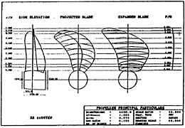
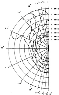
To investigate the validity of the present formulation in unsteady ship wake flow, we selected a 6300 TEU container ship propeller (HSVA Model 2395) whose geometrical particulars may be found in Figure 12. Figure 13 shows the nominal velocity contour measured at the towing tank of HSVA (Hamburg Ship Model Basin). Unfortunately the wake pattern at the HYKAT(HSVA large cavitation tunnel) is not measured. We use the model nominal wake for our computation.
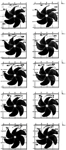
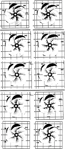
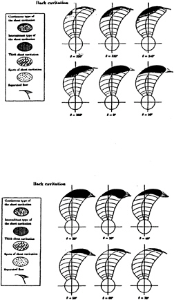
The time history of the cavitating pattern, computed with Δθp=6 deg. intervals, is shown at selected angular positions in Figure 14 for the container ship propeller with the cavitation number σn=1.7144, the Froude number Fn=2.4868 and the advance coefficient JA=0.7013. Experimental observations of the cavity extent at HYKAT are shown in Figure 15.
We observe that the predicted cavity extent is slightly larger than that observed. It should however be noted that the speed at the cavitation tunnel is about three times faster than that at the towing tank, and hence the boundary layer near the stern at HYKAT is considered thinner than the corresponding value at the towing tank. To find out the source of discrepancy between the tunnel result and the present prediction, further study is necessary with the wake measured directly at the cavitation tunnel.
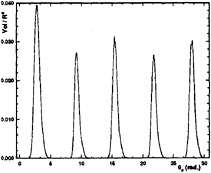
For the same case, Figure 16 shows the cavity volume variation for the first five revolutions of the propeller. We observe that the cavity volume variation in each cycle converges to an asymptote very rapidly. This cavity volume variation will be the most important information in judging the cavity influence upon the fluctuating pressures on an adjacent hull surface.
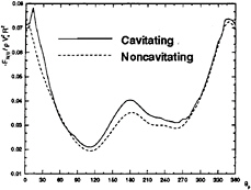
In Figure 17, the axial thrust variation under the cavitating condition is compared with the corresponding variation under the noncavitating condition. We observe that the loading on a cavitating propeller slightly increases due to the additional camber effect of the cavity.
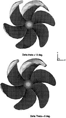
To check the influence of the angular step, we repeated the same computing but this time by doubling the angular step Δθp=12 deg, and compared with that obtained with 6 deg spacing, as shown in Figure 18. The two results are almost identical except the supercavity portion near the tip. This is caused by the longer panel size (doubled in chordwise direction). Although all the sample computations are made with finer angular step, 6 degree spacing is a good alternative in estimating the cavitation behavior at the initial design stage, since it reduces the CPU time by a factor of two.
5.5
Unsteady cavitation on propeller in screen-generated wake
Further computations are carried out with another propeller for which the wire-mesh generated wake data is available. The geometrical particulars of the Propeller KP325 may be found in Figure 19. Figure 20 shows the nominal velocity contour simulated at the KRISO cavitation tunnel for a 4400TEU container carrier.
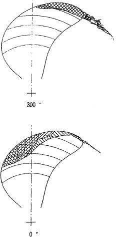
The time history of the cavitating pattern is shown at selected angular positions in Figure 21 with the cavitation number σn=2.04, the Froude number Fn=2.072 and the advance coefficient JA=0.7642. Experimental observations of the cavity extent at the KRISO cavitation tunnel are shown in Figure 22.
We observe that the correlation is very good, especially the close resemblance at the blade angle of 320 degrees when the cavity just starts. In general the predicted cavity extent is slightly larger than that observed. We expect that the correlation might be improved further once the effective velocity distribution is taken into consideration in the propeller-cavity analysis procedure.
6
Conclusions
A low order potential-based panel method is developed to treat the partial- or super-cavitating propellers operating in ship-generated wake.
The method is systematically validated through a series of tests varying the geometry from the simple 2-D profile to 3-D rectangular foil and propeller and also covering the steady and unsteady cavitation phenomena. The numerical formulation and procedure is evidenced robust and stable.
The cavity behavior predicted for the propeller operating behind a model ship and that operating in screen-generated wake shows good correlations with experiments.
The CPU for a typical six-bladed propeller is about 4 hours on the CRAY YMP2(16 GFLOPS) supercomputer for 5 rotations of propeller. This is the only drawback of the current procedure, which may still be considered to be a strong and reliable candidate to substitute the model experiments in saving the cost and time.
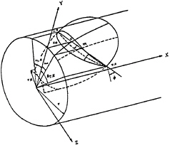
Figure 1: Coordinate system
References
[1] Kerwin, J.E. & Lee, C.-S., “Prediction of steady and unsteady marine propeller performance by numerical lifting surface theory,” Trans. SNAME, Vol. 86, 1978, pp. 218–258
[2] Lee, C.-S., “Prediction of steady and unsteady performance of marine propellers with or without cavitation by numerical lifting surface theory,” Ph.D. Thesis, M.I.T., Cambridge, Mass., 1979.
[3] Kinnas, S.A., “Leading edge correction to the linear theory of partially cavitating hydrofoils,” J. of Ship Research, Vol. 35, No. 1, March 1991, pp. 15–27.
[4] Lee, C.-S., “A potential-based panel method for the analysis of a 2-dimensional partially cavitating hydrofoil,” J. of Soc. of Naval Arch. of Korea(SNAK), Vol. 26, No. 4, 1989, pp. 27–34.
[5] Uhlman, J.S., “The surface singularity method applied to partially cavitating hydrofoils, ” J. of Ship Research, Vol. 31, No. 2, June 1987, pp. 107–124.
[6] Lee, C.-S., Kim, Y.-G. & Lee, J.-T., “A potential-based panel method for the analysis of a two-dimensional super- or partially cavitating hydrofoil,” J. of Ship Research, Vol. 36, No. 2, June 1992, pp. 168–181
[7] Morino, L. and Kuo, C.-C., “Subsonic potential aerodynamic for complex configurations: a general theory,” AIAA Journal, Vol. 12, No. 2, 1974, pp. 191–197.
[8] Kinnas, S.A. & Fine, N.E., “Nonlinear analysis of the flow around partially or supercavitating hydrofoils by a potential based panel method,” IABEM-90 Symposium of the International Association for Boundary Element Methods, Springler-Verlag, Rome, Italy, 1990, pp. 289–300.
[9] Kim, Y.-G., Lee, C.-S. and Suh, J.-C., “Surface panel method for prediction of flow around a 3-D steady or unsteady cavitating hydrofoil,” Cavitation '94, The Second International Symposium on Cavitation, Tokyo, Japan, 1994, pp. 113–120.
[10] Fine, N.E., “Nonlinear analysis of cavitating propellers in nonuniform flow,” Ph.D. Thesis, M.I.T., Cambridge, Mass., 1992.
[11] Kim, Y.-G., “Prediction of unsteady performance of marine propellers with cavitation using surface panel method,” Ph.D. Thesis, Chungnam National University, Taejon, Korea, 1995.
[12] Kim, Y.-G. and Lee, C.-S., “Prediction of unsteady cavity behavior around a 2-D hydrofoil in heave or gust,” The second Japan-Korea Joint Workshop on Ship and Marine Hydrodynamics , Osaka, Japan, June 28–30, 1993, pp.299–308.
[13] Boswell, R.J., “Design, cavitation performance, and open-water performance of a series of research skewed propellers,” DTNSRDC Report 3339, March 1971.
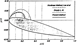
Figure 2: Comparison of cavity shapes predicted by linear and nonlinear theories for partial cavity
Figure 3: Comparison of cavity shapes predicted by linear and nonlinear theories for super-cavity
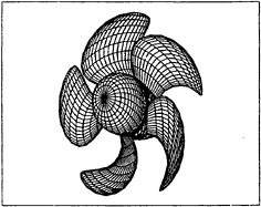
Figure 4: Quadrilateral representation of a propeller blade
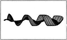
Figure 5: Nonlinear wake geometry
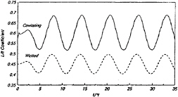
Figure 6: Lift coefficient variation with time for a partially cavitating hydrofoil in heave
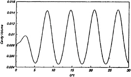
Figure 7: Cavity volume variation with time for a partially cavitating hydrofoil in heave
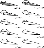
Figure 8: Cavity shape variation with time for a partially cavitating hydrofoil in heave; T=Period of heavig motion
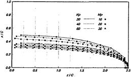
Figure 9: Convergence characteristics of cavity extent with the number of panels distributed on a rectangular hydrofoil
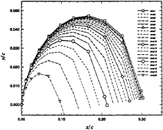
Figure 10: Cavity shape for a partially cavitating rectangular hydrofoil
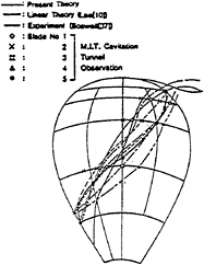
Figure 11: Comparison of cavity extent between predictions and observations for DTRC Propeller 4381 at JA=0.7 with σn=1.92
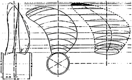
Figure 12: Drawing of 6300 TEU Propeller
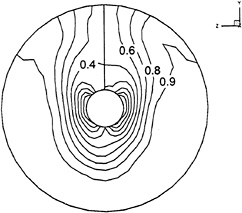
Figure 13: Iso-axial velocity (VA/Vs) contours of the wake measured at HSVA towing tank
DISCUSSION
S.A.Kinnas
University of Texas at Austin, USA
The authors should be commended for their efforts to implement a panel method for the prediction of unsteady propeller cavitation. A very similar method was presented at the 19th CNR Symposium on Naval Hydrodynamics (1992) by Kinnas and Fine. It would be interesting to hear the author's comments on the following issues:
-
How do they determine the cavity detachment point?
-
How do they plan to improve the slow convergence of the predicted cavity platform (see Fig.9)? In the work mentioned above we found that we had to develop a special treatment of the panel at which the cavity ends (the so-called “split-panel”) in order to improve the convergence.
-
From Figures 4 and 18 it appears that they have only used 10 panels in the spanwise direction. Has this been found to be sufficient for predicting the cavity shapes on the propeller, especially since they show that their predicted cavity shapes converge slowly with number of panels?
It would be nice to include in their reply a convergence study with number of panels for one of the propellers for which they compare their results with measurements.
AUTHORS' REPLY
NONE RECEIVED


