
2
Trends in Development Patterns
As a prelude to examining the relationship between land development patterns and vehicle miles traveled (VMT), this chapter provides background information on development patterns in the United States. It begins with a review of national and metropolitan area trends with respect to population and land development. The chapter then turns to an examination of spatial trends within metropolitan areas, the primary geographic focus of this study, including changes in population density and employment concentration over time, topics on which the most data are available. The chapter ends with findings concerning metropolitan development trends and their implications for travel.
NATIONAL AND METROPOLITAN AREA TRENDS IN POPULATION AND DEVELOPMENT
The U.S. census is the traditional source of long-term data on population trends by geographic area. Census data from 1970 to 2000 show that the U.S. population has continued to urbanize and suburbanize. As a share of total population, metropolitan population increased from 69 percent in 1970 to 80 percent in 2000 (Hobbs and Stoops 2002 in Giuliano et al. 2008, 11). Within metropolitan areas, however, the population has continued to suburbanize. From 1970 to 2000, the suburban population slightly more than doubled, from 52.7 million
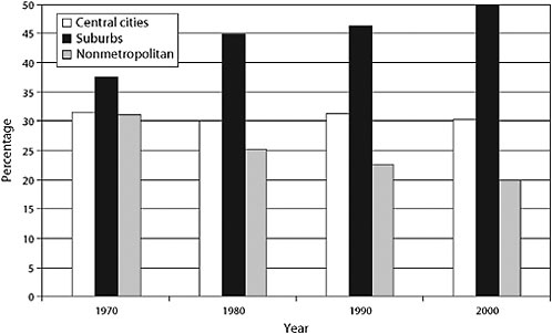
FIGURE 2-1 Percentage of total population living in central cities, suburbs, and nonmetropolitan areas, 1970–2000.
Source: Hobbs and Stoops 2002, 33, in Giuliano et al. 2008, 12.
to 113 million.1 This growth occurred mainly at the expense of non-metropolitan areas. Population in central cities grew, but only by about 55 percent, from 44 million to 68.5 million, while nonmetropolitan population declined from 63 million to 55.4 million (Giuliano et al. 2008, 11) (see Figure 2-1 for percentage changes). In terms of relative share, the suburban population increased from 54.5 percent of the total metropolitan area population in 1970 to more than 62 percent in 2000.
Jobs have followed population to the suburbs, although with a lag. In 1970, for example, 55 percent of jobs were still located in central cities (Mieszkowski and Mills 1993, 135). By 1990, that share had fallen to 45 percent.
|
1 |
The U.S. Bureau of the Census does not identify a location as “suburban.” Metropolitan areas are divided into two classifications: (a) inside central city and (b) outside central city. Many researchers treat the latter areas as suburban, and they are so treated in this report (see Giuliano et al. 2008, Appendix B). |
Another way to look at population and development trends is to focus on land development patterns and how they have changed over time, the principal concern of this study. According to the U.S. Department of Agriculture’s National Resources Inventory (NRI),2 between 1982 and 2003, an estimated 35 million acres of land (55,000 square miles) was developed in the United States—approximately one-third of all the land that had been developed by 2003.3 In all, 108.1 million acres was classified as developed in 2003—approximately 5.6 percent of the national total. Developed land grew at almost twice the rate of population over this 21-year period, clearly indicating that population densities were declining.4
Population and land development patterns, however, exhibit considerable variation across the United States. For example, some rapidly growing western states, such as California, Nevada, and Arizona, added population to their metropolitan statistical areas (MSAs) at a faster rate than they were spreading out (Fulton et al. 2001).5 At the same time, slowly growing MSAs of the northeast and midwest expanded in land area even as their population growth slowed or reversed. Overall, the northeast and midwest regions each gained about 7 percent in population, but their urbanized land increased by 39 and 32 percent,
respectively, between 1982 and 1997, the most recent year for which urbanized land data are available. In comparison, while the west and south gained 32 and 22 percent, respectively, in population, their land area grew by 49 and 60 percent, respectively (Fulton et al. 2001, 19). These data are too broad to ascertain whether MSA development is occurring in ways that could shorten automobile trips and support alternative modes of transportation. In the following section, spatial patterns of residential and employment development are examined at a finer geographic scale within metropolitan areas.
SPATIAL TRENDS WITHIN METROPOLITAN AREAS
Spatial trends within metropolitan areas encompass both the density and the location of development.
Density of Development
As noted in Chapter 1, density is one of the most commonly used measures to characterize development patterns. The level of density also has implications for travel. The length of trips taken in metropolitan areas with higher densities should be shorter than the length of those in areas with low densities, assuming that other built environment dimensions are the same. As density rises, trip origins become closer to trip destinations, on average. In addition, metropolitan areas with comparatively high average density tend to have centers where population and employment are dense enough to support transit service at levels that make it competitive with the automobile.
Density is often measured in terms of persons per square mile of total area within a city or county, as in the U.S. census. As noted in Chapter 1, however, this measure does not adequately capture development patterns, as some cities and counties contain large amounts of undeveloped land, while others are completely developed. Researchers employ several approaches to improve on this measure by using devel-
oped land on which people or jobs are located as the denominator. Fulton et al. (2001) use land-cover data from the NRI, for example, while Cutsinger and Galster (2006) set “extended urban area” (EUA) bound aries on the basis of census definitions and thresholds and identify developed and developable land within the EUAs to establish their denominator. Ewing et al. (2002) combine a series of density measures using both NRI and census results to create a standardized density index that forms one of four factors within their overall “sprawl” index.
On the basis of Fulton’s measure, of the 281 MSAs studied, density levels ranged from more than 20 persons per urbanized acre in New York and Jersey City to fewer than 2.5 persons per urbanized acre in Scranton, Charlotte, Knoxville, and Greenville–Spartanburg.6 The list of dense metropolitan areas—those over the 75th percentile density of 5.55 persons per urbanized acre—features a significant number of older metropolitan areas established before the advent of the automobile: the primary MSAs within metropolitan New York, San Francisco, Chicago, Buffalo, Providence, Washington, Boston, and New Orleans.7 But many areas that have experienced most of their growth since World War II also appear in this group, including Los Angeles–Long Beach (10.0 persons per urbanized acre), Anaheim–Santa Ana (9.2), San Jose (8.5), Las Vegas (6.7), and Phoenix (7.2). Perhaps more surprising, when considered over time, the fastest decline in density has not been occurring in areas often considered to be epicenters of sprawl. Las Vegas, Denver, Phoenix, and Riverside–San Bernardino, for example, all had population growth that exceeded growth in urbanized land according to the NRI data. Using other methods, Galster et al. (2001) and Ewing et al. (2002) confirm the relatively high density of California
metropolitan areas, Las Vegas, and Phoenix and the low density of metropolitan areas in the southeast.
Larger residential lot sizes are at least partly responsible for the rapid decline in density in some metropolitan areas. From 1987 to 1997, the density of the average urban acre declined from 1.86 dwelling units (DUs) per acre to 1.66 DUs per acre, largely because the new development over this period was built to a density of only 0.99 DUs per urban acre, bringing down the overall average.8 Recent results of the American Housing Survey, however, suggest a wide variation in lot sizes across metropolitan areas. For example, between 1998 and 2002, the median lot size for new one-family houses in the Anaheim– Santa Ana area (Orange County, California) was only 0.17 acre; in Portland (Oregon), 0.19 acre; and in Denver, 0.21 acre—all metropolitan areas defined as higher density. In Atlanta, a metropolitan area noted for its more dispersed land development patterns, the median lot size was 0.58 acre; in Hartford, at the extreme, it was more than 1.5 acres.
It is worth noting that a traditional rule of thumb for the density needed to support transit is 7 to 15 DUs per residential acre, or a gross density of more than 4,200 to 5,600 persons per square mile (Pushkarev and Zupan 1977, 177, in Downs 2004). No MSA in the country is that dense across its entire region, although for the 40 or so largest MSAs, areas within their boundaries exceed this minimum density. According to the 2000 U.S. census and the national database of the Center for Transit-Oriented Development, a total of about 14 million people, representing 6.2 million households, live within a half-mile radius
|
8 |
The density calculations are based on the NRI’s land-cover data, which were aggregated to correspond with U.S. census designations for metropolitan areas as defined in 1999. The NRI’s urban and built-up land category is used as the denominator, and intercensal estimates of housing units at the metropolitan level as the numerator. Changes in density are discussed in more detail in Chapter 5 and Appendix C. The reader should note that 0.99 DU per urban acre does not directly translate into residential lot sizes of 1 acre, nor is it equivalent to the lot sizes used in the American Housing Survey. NRI-defined urban acres include not only residential land but many other uses. See Appendix C, Box C-1, for more details. |
of existing fixed-route transit stations in the 27 metropolitan areas studied (Center for Transit-Oriented Development 2004, 18).9 The half-mile radius is considered to be a reasonable catchment area for having an impact on the travel behavior of area residents (i.e., encouraging a mode shift to transit).
Location of Development
The distribution of population and employment in a metropolitan area is determined by the relative strength of economies and diseconomies of agglomeration—the clustering of economic activities because of economies of scale, reduced transportation costs, and many other benefits.10 The standard monocentric urban model assumes the existence of an employment center, such as the central business district (CBD), and distributes households in relation to that center on the basis of trade-offs between the costs of housing and the costs of commuting (Anas et al. 1998 and Fujita 1989 in Giuliano et al. 2008). The model predicts declining and constantly decreasing population density the farther an area is from the CBD or city center as households face the trade-off between lower housing costs (land costs are lower farther from the city center) and higher commuting costs. Decentralization is accelerated by growth in real per capita income and declining unit (e.g., per mile) transportation costs as households seek to consume more housing and locate farther away from the city center (Mieszkowski and Mills 1993).
Researchers have employed many different measures to analyze the concentration (and dispersion) of both population and employment and clustering in centers, such as the CBD or newer suburban employment
centers.11 Centrality is a measure of the extent to which the development within a metropolitan area spreads out from a point of highest density. Closely related to centrality is the density gradient, a measure representing average density at increasing distances from the center.
Residential Location
As population density within some metropolitan areas has declined, so have density gradients. Kim (2007) analyzed population data for a consistent group of 87 cities with populations of at least 25,000 and their metropolitan areas from 1940 to 2000 to examine changes in population density and density gradients.12 He assumed a monocentric metropolitan area to estimate density gradients. He found that average population density levels have declined since 1950, and the estimated density gradient has declined consistently over the entire period studied (see Table 2-1). Kim suggests that the accelerated flattening of the density gradient since 1950 is likely due not only to the suburbanization of the population but also to the expansion of suburban land area, as found by Fulton et al. (2001). The rate of change in both average density levels and the density gradient appears to have begun slowing in the 1990s, but this trend cannot be definitively established because Kim’s city sample excludes cities that failed to meet the metropolitan area definitions of 1950.
Monocentric models and average measured density gradients, while reasonable for capturing broad trends in urban form, mask internal dynamics that may be more useful in ascertaining the evolution of
TABLE 2-1 Spatial Trends, Urban Population, 1940–2000
|
Year |
Central City– Metro Population Ratio |
Average Metro Density (persons per square mile) |
Density Gradient |
|||
|
Ratio |
Change |
Density |
Change |
Gradient |
Change |
|
|
1940 |
0.61 |
— |
8,654 |
— |
−0.72 |
— |
|
1950 |
0.57 |
−0.04 |
8,794 |
140 |
−0.64 |
−0.08 |
|
1960 |
0.50 |
−0.07 |
7,567 |
−1,227 |
−0.50 |
−0.14 |
|
1970 |
0.46 |
−0.04 |
6,661 |
−906 |
−0.42 |
−0.08 |
|
1980 |
0.42 |
−0.04 |
6,111 |
−550 |
−0.37 |
−0.05 |
|
1990 |
0.40 |
−0.02 |
5,572 |
−539 |
−0.34 |
−0.03 |
|
2000 |
0.38 |
−0.02 |
5,581 |
9 |
−0.32 |
−0.02 |
|
Source: Giuliano et al. 2008. Adapted from Kim 2007, 283. |
||||||
population and employment distributions within metropolitan areas (Giuliano et al. 2008). Nor do they provide a sufficiently detailed picture of the rich urban landscape. Outside the central city, density levels can vary greatly, from the generally more dense inner suburbs, to the very low densities of many outer suburbs, to housing complexes and communities of varying densities in between—all with different implications for travel and trip making.
Employment Location
In the field of economic geography, special attention has been paid to the location of employment, leading to the characterization of employment in metropolitan areas as monocentric, polycentric, or noncentered or dispersed (Lee 2007). The monocentric model has increasingly lost its explanatory power as employment has decentralized and the reasons for clustering in a single CBD have diminished (see Clark 2000 in Lee 2007). Two competing views have emerged with regard to the implications
of this decentralization for urban form. The first and dominant view, according to Lee (2007), holds that metropolitan areas are polycentric, increasingly characterized by the presence of multiple activity nodes or employment centers. The second view (Glaeser and Kahn 2001; Lang and LeFurgy 2003) holds that suburban employment should be conceived of as being dispersed, not polycentered (Glaeser and Kahn 2001). Lang and LeFurgy (2003) provide data that support the second view, at least as it relates to the dispersion of office space. In 13 of the nation’s largest office markets, for example, most metropolitan rental office space exists either in high-density downtowns or in low-density edgeless cities, not in employment centers outside the CBD.13
Understanding employment patterns, particularly the factors that lead to the formation of employment centers outside the CBD, has particular relevance for the present study. Travel patterns are influenced by the density of commercial as well as residential development, particularly the density of development at the job end of the daily commute (Cervero and Duncan 2006). Of particular interest is whether jobs are clustering outside of the center city in aggregations large enough to support transit; encourage mixed-use development near job sites within walking distance; or facilitate shorter automobile trips because jobs are located closer to residents, thereby improving the jobs–housing balance.
A review of the literature in a paper commissioned for this study (Giuliano et al. 2008) finds support for the view that decentralization of employment in metropolitan areas has resulted in new agglomerations outside the CBD. The presence of employment centers is demonstrated across metropolitan areas of varying size, age, location, and growth rates (see Table 8 and discussion in Giuliano et al. 2008). Nevertheless, the authors note that, despite the presence of these centers, most metropolitan employment is dispersed; the share of employment outside centers is on the order of two-thirds to three-fourths (Giuliano
et al. 2008, 32). The authors conclude, however, that this finding fails to support the view that today’s metropolitan areas are better described as dispersed; rather, they exhibit both employment concentrations and dispersion.14
Only a handful of studies could be found that examine trends in employment patterns over time. The first, by Lee (2007), uses a series of centralization and concentration indices to examine patterns of employment change in six large metropolitan areas, from 1980 to 2000 for San Francisco and Philadelphia and from 1990 to 2000 for New York, Los Angeles, Boston, and Portland. Lee reports that development trends reinforced the polycentricity of Los Angeles and San Francisco, as a significant proportion of decentralizing jobs reconcentrated in suburban centers, but concludes that California metropolitan areas are not typical. Philadelphia, Portland, New York, and Boston are more monocentric, with the CBD housing a larger proportion of all center employment. Nevertheless, the CBDs of Philadelphia and Portland lost share; jobs dispersed without significant suburban clustering. In comparison, the well-established CBDs of Boston and New York were better able to retain their strength as city centers even as growth occurred on their peripheries.
Lee concludes that job dispersion is occurring as jobs continue to decentralize to the suburbs. However, he notes remarkable variation in spatial trends and evidence of suburban agglomerations just among the six metropolitan areas studied. He attributes the differences to history, topography, and the requirements of different economic sectors. Cities like New York, Boston, and Philadelphia, whose core areas were developed before the 20th century, have retained more of their monocentric character and radial development patterns, the result of path-dependent growth and the durability of the built environment.
Portland’s monocentricity can best be explained by its relatively small size. And the polycentric character of San Francisco and Los Angeles is reinforced by their history and topography.
The second study is a case study of the Los Angeles metropolitan area, focused on the urbanized area portion of the five-county Los Angeles consolidated MSA (CMSA), comprising Los Angeles, Orange, Riverside, San Bernardino, and Ventura Counties (Giuliano et al. 2008). The researchers found evidence of both decentralization and deconcentration of employment.15 The share of jobs in the densest 10 percent of land area declined from about 84 percent in 1980 to 71 percent in 2000 (Giuliano et al. 2008, 21). Employment concentrations also decentralized; the average (employment-weighted) distance of all census tracts to tracts with at least 20 jobs per acre increased from 8.3 miles in 1980 to 11 miles. Nevertheless, overall the region’s employment remained highly concentrated. While Los Angeles County lost jobs between 1990 and 2000, it still housed the largest number of jobs in 2000 by nearly a factor of three compared with Orange County, which had the next highest employment level. Furthermore, employment centers grew over the period, from 36 centers identified in the 1980 data to 46 and 48 centers in 1990 and 2000, respectively (Giuliano et al. 2008, 21).16 The share of county employment in centers remained steady in Los Angeles County but increased in Orange County, particularly in suburban areas northwest and southeast of the Los Angeles CBD that had become more urban over this period. In contrast, the outer suburbs are in a different stage of development and exhibited rapidly growing but dispersed employment.
The authors also examined the impact of employment distribution on travel patterns, of particular interest to the present study. They found considerable variation in the economic characteristics and design of employment centers that affect commuting, particularly by transit. For example, the Los Angeles CBD is a mixed-use area with high average employment density and a transit system focused on the downtown, accounting for its high transit share (see Table 18 in Giuliano et al. 2008). In contrast, the Santa Ana–Irvine center, which is located around the Orange County airport, stands out for its high drive-alone share, reflecting its emergence around several major freeways and its automobile-oriented design. These examples illustrate the importance of employment center characteristics for travel behavior.
A third study (Lee et al. 2006) examines the employment trends and commuting patterns of 12 CMSAs from 1980 to 1990. The highest-growth CMSAs had the highest employment growth, but in all cases the total share of jobs in the central city declined (see Table 2-2).17 Some cities fared better than others. New York and Chicago, for example, had minor share losses. In Denver, the central city share of employment dropped by 10 percentage points between 1980 and 1990. Cleveland and Detroit also registered substantial employment losses in the central city in what has come to be called a “hollowing out” phenomenon.
Changes in commuting patterns generally reflect differences in high-growth versus slow-growth cities. In all the CMSAs, the share of suburb-to-suburb commuting increased, while all other shares decreased (Lee et al. 2006 in Giuliano et al. 2008). CMSAs in the south and west had the greatest increase in commute flows, reflecting their more rapid growth and higher share of suburb-to-suburb commutes, and many showed resulting increases in average travel times. In contrast, longer travel times for suburb-to-suburb commutes in CMSAs in the northeast and midwest were partially offset by shorter
TABLE 2-2 Employment Trends Inside and Outside the Central City, 1980–1990
travel times in other categories, reducing the increase in metropolitan area averages.
Two other studies explore changes in the jobs–housing balance in metropolitan areas and how these changes have affected commuting travel. Horner (2007) examines changes in the relative distribution of workers and jobs in the Tallahassee metropolitan area between 1990 and 2000. He reports that the proximity of workers and jobs declined over the period with the decentralization of jobs. The actual average commute distance, however, increased by only 0.3 mile. Horner attributes this result in part to job adjustments by workers and to efforts of land regulators and developers to maintain a good jobs–housing balance (Horner 2007 in Giuliano et al. 2008). Data are not available with which to determine the number of workers living in a zone who actually work in that zone, which could partially explain the lack of change in commute distance.
Yang (2008) conducted a similar study of Boston, a relatively compact metropolitan area, and Atlanta, a lower-density metropolitan area without strong transit and with few mixed-use areas, to examine changes in the distribution of workers and jobs from 1980 to 2000. The average commute time and distance were shorter in Boston than in Atlanta, reflecting the greater proximity of jobs and housing in the former. Both areas showed an increase in the distance between the average resident and the average job over the period, but this increase did not translate into significantly longer commute distances. During the period, estimated actual average commute distances increased by about 3 miles in Boston and about 2.25 miles in Atlanta (Giuliano et al. 2008, 19).18
A final study—an analysis of metropolitan employment trends from 1998 to 2006 that builds on the work of Glaeser and Kahn (2001)— found that employment has continued to decentralize (Kneebone 2009).
Private-sector jobs in 95 of the 98 largest metropolitan areas studied saw a decrease in the share of jobs located within 3 miles of a downtown.19 Although the 98 metropolitan areas experienced a 10 percent overall increase in the number of jobs within 35 miles of downtown, the urban core saw an increase of less than 1 percent; the middle (3 to 10 miles) and outer (more than 10 to 35 miles) rings saw increases of 9 percent and 17 percent, respectively (Kneebone 2009).20 As of 2006, approximately one-fifth (21 percent) of employees in the top 98 metropolitan areas worked within 3 miles of a downtown; more than twice that share (45 percent) worked more than 10 miles from the city center. The larger the metropolitan area, the more likely people were to work more than 10 miles away from the downtown. Type of industry also mattered. More than 30 percent of jobs in utilities and in financial and insurance and educational services were located within the urban core, while about half the jobs in manufacturing, construction, and retail were located more than 10 miles away (Kneebone 2009). The author concludes that the dominant trend during the study period was further dispersion of jobs toward the metropolitan fringe. The study, however, was not designed to examine the extent to which suburban employment centers were forming outside the CBD during the period.
FINDINGS AND IMPLICATIONS FOR TRAVEL
The data presented in this chapter support the finding that while the majority of the U.S. population (80 percent in 2000) lives in metropolitan areas, population and employment have continued to suburbanize.
This trend threatens to reduce densities below levels that may be needed to support alternatives to the automobile, such as transit, and result in longer automobile trips.
To a large extent, these concerns are borne out by the data. In many MSAs, developed land is increasing more rapidly than population, population density gradients are continuing to decline, and the share of employment in the central city is falling. However, the data also show some encouraging trends with respect to both population and employment. With regard to the former, an increasing share of the U.S. population lives in metropolitan rather than in nonmetropolitan areas. In addition, there is some evidence that the decline in population density is attenuating. Some metropolitan areas in California, Nevada, and Arizona, for example, are surprisingly dense and becoming more so.
With regard to employment, the suburbanization of employment as well as residences may help reduce trip lengths by improving the jobs– housing balance, although the evidence is difficult to identify directly with current data sources. In some metropolitan areas, central cities appear to be retaining their share of total employment; this is particularly true for older metropolitan areas, such as New York and Boston, with relatively large central cities. Although metropolitan employment is dispersed, the presence of new agglomerations or suburban employment centers outside the CBD is evident in metropolitan areas of varying size, age, location, and growth rates. In some metropolitan areas, the share of suburban employment in centers appears to be increasing.
The implications of these development trends for travel are difficult to determine. The lack of fine-grained geographic data and longitudinal studies of population and employment changes within metropolitan areas limits our ability to understand spatial development patterns at the level necessary to determine effects on trip making, mode choice, and VMT. The key is to know how densely developed neighborhoods and job centers need to become and how they should be designed or redesigned to reduce VMT and encourage nonautomotive trips. The next chapter examines what is known from the literature about the relationship
between development patterns—in particular more compact, mixed-use development; better jobs–housing balance; and good transit service— and VMT and mode choice.
REFERENCES
Abbreviations
NRCS National Resources Conservation Service
OMB Office of Management and Budget
Anas, A., R. Arnott, and K. A. Small. 1998. Urban Spatial Structure. Journal of Economic Literature, Vol. 36, No. 3, pp. 1426–1464.
Center for Transit-Oriented Development. 2004. Hidden in Plain Sight, Capturing the Demand for Housing near Transit. Reconnecting America, Oakland, Calif.
Cervero, R., and M. Duncan. 2006. Which Reduces Vehicle Travel More: Jobs–Housing Balance or Retail–Housing Mixing? Journal of the American Planning Association, Vol. 72, No. 4, pp. 475–490.
Clark, W. A. 2000. Monocentric to Polycentric: New Urban Forms and Old Paradigm. In A Companion to the City (G. Bridge and S. Watson, eds.), Blackwell Publishing, Inc., Oxford, United Kingdom, pp. 141–154.
Cutsinger, J., and G. Galster. 2006. There Is No Sprawl Syndrome: A New Typology of Metropolitan Land Use Patterns. Urban Geography, Vol. 27, No. 3, pp. 228–252.
Downs, A. 2004. Still Stuck in Traffic: Coping with Peak-Hour Traffic Congestion. Brookings Institution, Washington, D.C.
Ewing, R., R. Pendall, and D. Chen. 2002. Measuring Sprawl and Its Impact. Smart Growth America. www.smartgrowthamerica.org/sprawlindex/MeasuringSprawl.pdf. Accessed Aug. 20, 2008.
Fujita, M. 1989. Urban Economic Theory: Land Use and City Size. Cambridge University Press, Cambridge, United Kingdom.
Fulton, W., R. Pendall, M. Nguyen, and A. Harrison. 2001. Who Sprawls Most? How Growth Patterns Differ Across the U.S. Survey Series. Brookings Institution, Washington, D.C.
Galster, G., R. Hanson, M. Ratcliffe, H. Wolman, S. Coleman, and J. Freihage. 2001. Wrestling Sprawl to the Ground: Defining and Measuring an Elusive Concept. Housing Policy Debate, Vol. 12, pp. 681–718.
Giuliano, G., A. Agarwal, and C. Redfearn. 2008. Metropolitan Spatial Trends in Employment and Housing: Literature Review. School of Policy, Planning, and Development, University of Southern California. http://onlinepubs.trb.org/Onlinepubs/sr/sr298giuliano.pdf.
Giuliano, G., and K. Small. 1991. Subcenters in the Los Angeles Region. Regional Science and Urban Economics, Vol. 21, No. 2, pp. 163–182.
Glaeser, E. L., and M. E. Kahn. 2001. Decentralized Employment and the Transformation of the American City. Working Paper 8117. National Bureau of Economic Research, Cambridge, Mass.
Hobbs, F., and N. Stoops. 2002. Demographic Trends in the 20th Century. Census 2000 Special Reports, Series CENSR-4. U.S. Government Printing Office, Washington, D.C.
Horner, M. 2007. A Multi-scale Analysis of Urban Form and Commuting Change in a Small Metropolitan Area (1990–2000). Annals of Regional Science, Vol. 41, pp. 315–352.
Kim, S. 2007. Changes in the Nature of Urban Spatial Structure in the United States, 1890–2000. Journal of Regional Science, Vol. 47, No. 2, pp. 273–287.
Kneebone, E. 2009. Job Sprawl Revisited: The Changing Geography of Metropolitan Employment. Metropolitan Policy Program. Brookings Institution, Washington, D.C.
Lang, R. E., and J. LeFurgy. 2003. Edgeless Cities: Examining the Noncentered Metropolis. Housing Policy Debate, Vol. 14, No. 3, pp. 427–460.
Lee, B. 2007. “Edge” or “Edgeless” Cities? Urban Spatial Structure in U.S. Metropolitan Areas, 1980–2000. Journal of Regional Science, Vol. 47, No. 3, pp. 479–515.
Lee, S., J. Seo, and C. Webster. 2006. The Decentralizing Metropolis: Economic Diversity and Commuting in U.S. Suburbs. Urban Studies, Vol. 43, No. 13, pp. 2525–2549.
Mieszkowski, P., and E. Mills. 1993. The Causes of Metropolitan Suburbanization. Journal of Economic Perspectives, Vol. 7, No. 3, pp. 135–147.
NRCS. 2002. National Resources Inventory 2002 and 2003 Annual NRI. U.S. Department of Agriculture, Washington, D.C. www.nrcs.usda.gov/technical/NRI/2002/glossary.html. Accessed Aug. 28, 2008.
NRCS. 2007. Natural Resources Inventory, 2003 Annual NRI, Land Use. U.S. Department of Agriculture, Washington, D.C.
OMB. 2000. Standards for Defining Metropolitan and Micropolitan Statistical Areas. Federal Register,Vol. 65, No. 249, pp. 82228–82238.
Pushkarev, B. S., and J. M. Zupan. 1977. Public Transportation and Land Use Policy. Indiana University Press, Bloomington.
U.S. Bureau of the Census. 2008. The 2009 Statistical Abstract, Table 2. Population: 1960 to 2007. www.census.gov/compendia/statab/. Accessed Feb. 26, 2009.
Yang, J. 2008. Policy Implications of Excess Commuting: Examining the Impacts of Changes in U.S. Metropolitan Spatial Structure. Urban Studies, Vol. 45, No. 2, pp. 391–405.


