
4
Observing the Active Earth: Current Technologies and the Role of the Disciplines
Not long ago, seismologists worked in rooms filled with drum recorders and big tables for hand-measuring seismograms. They now use digital monitoring systems that integrate high-performance seismometers, real-time communications, and automatic processing to produce high-quality information on seismic activity in near real time. Geodesists have replaced the theodolite and spirit level with space-based positioning and deformation imaging that can map crustal movements precisely and continuously, and they can hunt for slow, silent earthquakes with arrays of sensitive, stable strainmeters. Geologists have learned to decipher the subtle features of the rock record that mark prehistoric earthquakes, and they can date these events precisely enough to reconstruct the space-time behavior of entire fault systems. Laboratory and field scientists who study the microscopic processes of rock deformation are now formulating and calibrating the scaling laws that relate their reductionistic approach to the nonlinear dynamics of macroscopic faulting in the real Earth.
In each of these four domains—seismology, geodesy, geology, and rock mechanics—key technological innovations and conceptual breakthroughs were made within the last decade. The Global Seismic Network (GSN), initiated with the founding of the National Science Foundation (NSF)-sponsored Incorporated Research Institutions for Seismology (IRIS) in 1984, is reaching its design goal of 128 broadband, high-dynamic-range stations (as of December 2001, 126 stations had been installed and 122 were operational). The first continuously recording network of Global Positioning System (GPS) stations for measuring tectonic deformation
was installed in Japan in 1988 by the National Research Institute for Earth Science and Disaster Prevention (1), and the first image of earthquake faulting using interferometric synthetic aperture radar (InSAR) was constructed in 1992. Paleoseismologists produced a preliminary 1000-year history of major ruptures on the San Andreas fault in 1995 and discovered a prehistoric moment magnitude (M) 9 earthquake in the Cascadia subduction zone in 1996. The first three-dimensional simulations of dynamic fault ruptures using laboratory-derived, rate- and state-dependent friction equations were run in 1996.
The unprecedented flow of new information opened by these advances is stimulating research on many fronts, from fault-system dynamics and earthquake forecasting to wavefield modeling and the prediction of strong ground motions. This chapter summarizes the state of the art in the main observational disciplines; it focuses on new technologies for observing the active Earth, and it highlights through a few examples the richness of the data sets now becoming available for basic and applied research.
4.1 SEISMOLOGY
Seismology lies at the core of earthquake science because its main concern is the measurement and physical description of ground shaking. The central problem of seismology is the prediction of ground motions from knowledge of seismic-wave generation by faulting (the earthquake source) and the elastic medium through which the waves propagate (Earth structure). In order to do this calculation (forward problem), information must be extracted from seismograms to solve two coupled inverse problems: imaging the earthquake source, as represented by its space-time history of faulting, and imaging Earth structure, as represented by three-dimensional models of seismic-wave speeds and attenuation parameters. Because seismic signals can be recorded over such a broad range of frequencies—up to seven decades (2)—seismic signals can be used to observe earthquake processes on time scales from milliseconds to almost an hour, and they provide information about elastic structure at dimensions ranging from centimeters to the size of the Earth itself.
Seismometry
Seismic waves span a wide range of amplitude, as well as frequency. The ground motions in the vicinity of a large earthquake can have velocities greater than 1 meter per second and accelerations exceeding the pull of gravity (1g = 9.8 m/s2). The lower limit of seismic detection is typically eight orders of magnitude smaller, set by the level of the ambient ground
noise (3). No single sensor has yet been developed that can faithfully record the violent displacements close to an earthquake and still be capable of detecting small events at the background noise level. For this reason, instruments historically have been divided into weak-motion and strong-motion seismometers. The former have been the principal sensors for studies of Earth structure and remote earthquakes by seismologists (4), while the latter have provided the principal seismological data to earthquake engineers. Technology is closing this gap. Modern force-feedback systems (5) can faithfully record ground motions from the lowest ambient noise at quiet sites to the largest earthquakes at teleseismic distances and achieve a bandwidth that extends from free oscillations with periods of tens of minutes to body waves with periods of tenths of seconds (Figure 4.1).
Seismic Monitoring Systems
Seismic monitoring systems comprise three basic elements: a network of seismometers that convert ground vibrations to electrical signals, communication devices that record and transmit the signals from the stations to a central facility, and analysis procedures that combine the signals from many stations to identify an event and estimate its location, size, and other characteristics. Monitoring systems are multiple-use facilities; they furnish information about earthquakes and nuclear explosions to operational agencies in near real time, and they also function as the basic data-gathering mechanisms for long-term research and education. With current technology, seismic networks of different types and spatial scales must be deployed to register the Earth’s seismicity over its complete geographic and magnitude range (Table 4.1, Figure 4.2). Since this coverage is typically overlapping, monitoring systems can be effectively organized into nested structures.
Global Seismic Networks State-of-the-art seismic stations for global seismic networks comprise three-component sensors with high dynamic
TABLE 4.1 Scales of Seismic Monitoring
|
Type |
Typical Network Size |
Typical Station Spacing |
Detection Thresholda |
|
Global |
Global |
1000 km |
4.5 |
|
Regional |
500 km |
25-50 km |
2.0 |
|
Local |
10 km |
<1000 m |
–1.0 |
|
aMagnitude of smallest event with a high probability of detection; see examples in Figure 4.2. |
|||
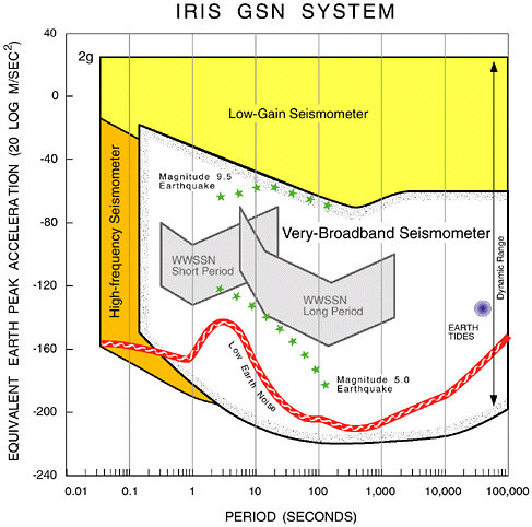
FIGURE 4.1 Plot of acceleration amplitude versus frequency, showing effective bandwidth and dynamic range for current broadband, high-frequency, and low-gain (strong-motion) digital seismometers, as well as for the older short-period and long-period analog seismometers of the World Wide Standardized Seismographic Network. Broadband instruments are capable of faithfully recording ground motions ranging from ambient noise at quiet sites (line labeled low Earth noise) to the peak accelerations generated by an M 9.5 earthquake at an epicentral distance of 3000 kilometers (upper line of stars). Low-gain seismometers are needed to record ground accelerations in the damage zones of large earthquakes, which can exceed 1g, and high-frequency seismometers are needed for periods less than about 0.1 second. SOURCE: R. Butler, IRIS.
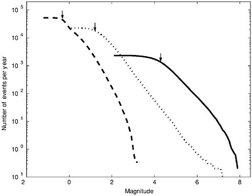
FIGURE 4.2 Number of earthquakes per year greater than a specified magnitude recorded by three networks of the types described in Table 4.1. Solid line shows the seismicity of the entire Earth from the global network of seismic stations cataloged by the International Seismological Centre during the decade 1990-1999. Dotted line is for events in southern California during the same interval recorded by the Southern California Seismic Network. Dashed line is for mining-induced seismicity recorded during 1997-1999 by a local network in the Elandrands gold mine, South Africa. Arrows show the approximate detection thresholds for the three networks, below which the sampling of seismicity is incomplete. All magnitudes are moment magnitudes. SOURCE: M. Boettcher, E. Richardson, and T.H. Jordan, University of Southern California.
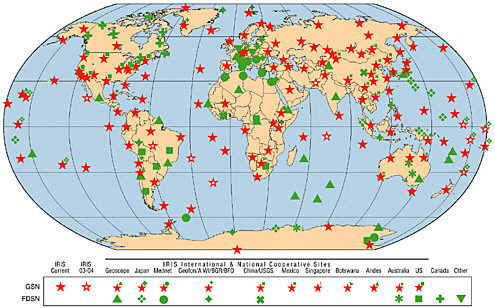
range (up to 140 decibels) and broadband response (0.0001–10 hertz). Since 1984, more than 300 such stations have been installed at permanent locations worldwide, as elements of global and regional networks (Figure 4.3). Close to half of these stations are part of the GSN, which has been constructed and operated under a cooperative agreement between the U.S. Geological Survey (USGS) and IRIS (6). The GSN is coordinated with other international networks through the Federation of Digital Seismographic Networks (FDSN), and the data are archived and made available
on-line by the IRIS Data Management Center (DMC) in Seattle, Washington (7). Some stations still record on local magnetic or optical media that are shipped periodically to the DMC, but direct telemetry is being deployed as communication with remote sites becomes cheaper. At many locations with telephone access, the data can be retrieved via telephone dial-up or Internet connection (108 stations in 2001). The five-year goal is to have all stations on-line all the time. Achieving this goal, especially at remote sites, will depend in part on the cost of satellite communications.
The GSN data acquired over the last 15 years have facilitated many advances in the study of global Earth structure and earthquake sources. Seismic tomography has provided dramatic images of subducting slabs, plume-like upwellings, and other features of the mantle convective flow responsible for plate-tectonic motions (Figure 4.4). The GSN data have also improved the plate-tectonic framework for understanding earthquake hazards through better earthquake locations and centroid moment tensor (CMT) solutions (Figure 4.5). Seismologists have used the broadband waveforms to elucidate the details of rupture processes during large earthquakes from a variety of tectonic settings, shedding new light on the geologic and dynamic factors that govern the configuration of seismogenic zones and how earthquakes start and stop.
These successes have in no way diminished the need for continued monitoring. Discoveries based on data now being collected by the GSN will undoubtedly continue into the indefinite future. On the rapidly slipping plate boundaries, large earthquakes recur at intervals ranging from decades to centuries, while the recurrence times for significant intraplate events can extend to many millennia. With each passing year, GSN data will thus add new information to the evolving pattern of global seismicity by the direct observation of large, rare events and the delineation of low-level seismicity that may mark the eventual occurrence of such events. The densification of seismic sources through time will also improve tomographic mapping of features in the crust and mantle that control seismicity and may be indicative of the forces causing lithospheric faulting.
Global seismological monitoring could be further enhanced by increasing the spatial resolution on land with permanent and temporary deployments of seismometers, expanding the coverage of global networks to the ocean floor, and upgrading the present networks as new technologies become available. However, sustained funding of the global networks will present a continuing challenge. In terms of annualized expenditures, the operation and maintenance of the GSN is projected to be comparable to its initial capitalization. Under current arrangements, the USGS shares a portion of the costs of GSN operations with the NSF. Stable support of the GSN from a federal agency that embraces the mission of global seismic monitoring is essential to the long-term health of earthquake science.
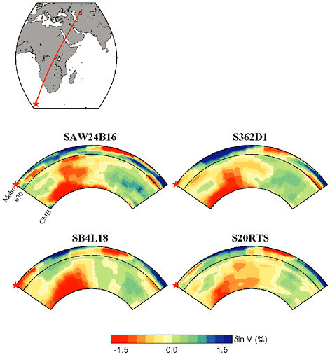
FIGURE 4.4 Depth cross section showing the African plume as seen in four recent global tomographic models of S velocity: SAW23B16 (Megnin and Romanowicz, 2000), SB4L18 (Masters et al., 1999), S362D1 (Gu et al., 2001), and S20RTS (Ritsema et al., 1999). Although the models differ in detail, they are in agreement on the broad characteristics of this major upwelling. SOURCE: Y.J. Gu, A.M. Dziewonski, W.-J. Su, and G. Ekström, Models of the mantle shear velocity and discontinuities in the pattern of lateral heterogeneities, J. Geophys. Res., 106, 11,169-11,199, 2001; G. Masters, H. Bolton, and G. Laske, Joint seismic tomography for P and S velocities: How pervasive are chemical anomalies in the mantle? Eos, Trans. Am. Geophys. Union, 80, S14, 1999; C. Megnin and B. Romanowicz, The 3D shear velocity structure of the mantle from the inversion of body, surface and higher mode waveforms, Geophys. J. Int.,143, 709-728, 2000; J. Ritsema, H. van Heijst, and J. Woodhouse, Complex shear wave velocity structure imaged beneath Africa and Iceland, Science, 286, 1925-1928, 1999. SOURCE: B. Romanowicz and Y. Gung, University of California, Berkeley.
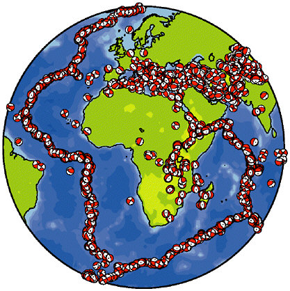
FIGURE 4.5 25 years of CMT solutions (1976-2000) for the region surrounding Africa. The availability of broadband data has made it possible to describe global seismicity in terms not only of location and magnitude, but also of fault mechanism, thereby greatly enhancing our view of active tectonics. SOURCE: Harvard CMT group.
Regional Seismic Networks Owing to their sparse station coverage, global networks do a poor job of detecting and locating events with magnitudes less than about 4.5 (Figure 4.2), and their sampling is too crude for investigating how waves are produced by fault ruptures, especially the near-fault radiation that generates the complex patterns of strong ground motions observed in large earthquakes. To deal with these problems, seismologists have densified station arrays in areas of high (or otherwise interesting) seismicity. Regional networks are collections of seismographic stations distributed over tens to hundreds of kilometers, usually as permanent facilities. The information supplied by regional networks services three overlapping but distinct communities: (1) scientists and engineers
engaged in basic and applied research; (2) engineers, public officials, and other decision makers charged with the management of earthquake risk and emergency response; and (3) public safety officials, news media, and the general public. As information technology has transformed the regional networks into integrated monitoring systems, they have become centers for educating the general public about earthquake hazards, as well as key facilities for training graduate students in seismology (8).
The short-period, high-gain instruments historically used in regional networks (9) brought seismicity patterns into much clearer focus (Figure 4.6), but the dynamic range of these instruments was too low to furnish useful recordings of large regional events. In the last decade, deployments of broadband, high-dynamic-range seismometers have begun to transform the regional networks into much more powerful tools for investigating the basic physics of the earthquake source, the detailed structure of the Earth’s crust and deep interior, and the patterns of potentially destructive ground motions. With these data, seismologists can now map the patterns of slip during earthquakes using seismic tomography, just as they map Earth structure. Images of fault ruptures during the more recent earthquakes in the Los Angeles, San Francisco, and Seattle regions have all been captured by high-performance networks (Figure 4.7).
Long-term funding has been a persistent problem for regional network operators, and new investments in equipment are badly needed (10). In particular, the implementation of new broadband technologies in regional monitoring has been lagging in the United States, especially when compared to the investments made by other high-risk countries such as Japan (Box 4.1) and Taiwan. Two exceptions are the Berkeley Digital Seismic Network in northern California and Caltech’s TERRAscope Network in southern California. Both are equipped with a combination of three-component broadband seismometers and three-component strong-motion accelerometers; they have digital station processors and feed continuous data streams via real-time telemetry to central processing sites. Although these networks have developed independently, a major effort is under way, with some support from the State of California, to modernize the earthquake monitoring infrastructure throughout the region by integrating the regional networks into a California Integrated Seismic Network monitoring in the United States.
Local Networks Networks have been deployed with seismometers distributed over a few tens of kilometers or less for specialized purposes such as seismic monitoring of critical facilities (e.g., dams and nuclear power plants) or localized source zones (e.g., volcanoes or geothermal reservoirs). Local networks are important instruments for the study of natural earthquake laboratories such as deep mines. Digital arrays of very
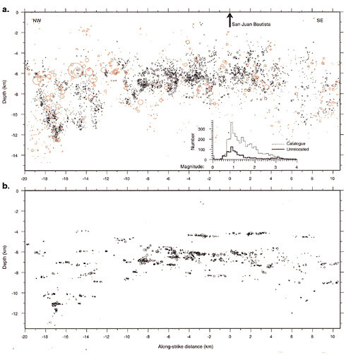
FIGURE 4.6 Vertical along-strike cross sections of earthquakes located along a 30-kilometer section of the San Andreas fault. Circles are an estimate of event size. (a) Locations of earthquakes between May 1984 and December 1997 reported in the Northern California Seismic Network catalog. (b) Relocated earthquakes show a linear, nearly horizontal pattern of seismicity. SOURCE: A.M. Rubin, D. Gillard, and J.-L. Got, Streaks of microearthquakes along creeping faults, Nature, 400, 635-641, 1999. Reprinted by permission from Nature copyright 1999 Macmillan Publishers Ltd.
high frequency sensors have been deployed in deep mines in Canada, Poland, and South Africa to monitor mine tremors and rock bursts induced by mining activities (11), and they have furnished unique, close-in observations of earthquakes as large as M 5 and at depths as great as 4 kilometers. Recent research has shown that in the deep gold mines of South Africa, mine tremors caused by friction-controlled slip on faults
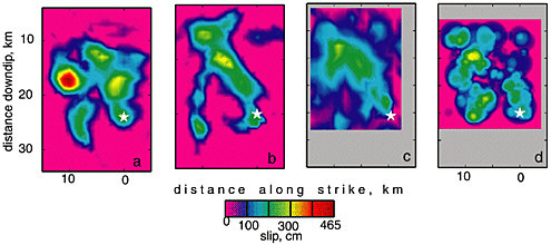
FIGURE 4.7 Comparison of fault slip maps for the 1994 Northridge earthquake derived from different methods. (a) Inversion of regional distance broadband data (Dreger, 1997). (b) Inversion of seismic moment rate functions derived from empirical Green’s function deconvolution (Dreger, 1994). (c) Inversion of local strong motion, teleseismic waveform data, and geodetic and leveling data (Wald et al., 1996). (d) Inversion of strong motion data alone (Zeng and Anderson, 1996). Each map has the same scaling, and the white star identifies the hypocenter. SOURCE: D. Dreger, Empirical Green’s Function study of the January 17, 1994 Northridge, California earthquake, Geophys. Res. Lett., 21, 2633-2636, 1994; D. Dreger, The large aftershocks of the Northridge earthquake and their relationship to mainshock slip and fault zone complexity, Bull. Seis. Soc. Am., 87, 1259-1266, 1997; D.J. Wald, T.H. Heaton, and K.W. Hudnut, The slip history of the 1994 Northridge, California, earthquake determined from strong-motion, teleseismic, GPS, and leveling data, Bull. Seis. Soc. Am., 86, S49-S70, 1996; Y. Zeng and J.G. Anderson, A composite source modeling of the 1994 Northridge earthquake using Genetic Algorithm, Bull. Seis. Soc. Am., 86, 71-83, 1996. SOURCE: D. Dreger, University of California, Berkeley.
|
BOX 4.1 Seismic Infrastructure in Japan Japan has been at the forefront of seismic monitoring since instrumental observations of earthquakes began in the 1870s. The Japan Meteorological Agency (JMA) operates a national network that provides essential data for the study of earthquake sources and seismotectonics throughout the Japanese islands.1 A number of local networks are operated by universities and other institutions, such as the National Research Institute for Earth Science and Disaster Prevention of the Science and Technology Agency, primarily for research on microseismicity and earthquake prediction. The Earthquake Prediction Data Center of the Earthquake Research Institute, University of Tokyo, receives hypocenter and arrival-time data from member universities and compiles them into two databases, one for real-time analysis and a revised one for archival purposes. More than 700 stations are currently operational, making the detection and location of all earthquakes of M > 2 possible almost everywhere in the country. A distinctive feature of earthquake monitoring in Japan has been the systematic collection of observations on the intensity of seismic shaking, a tradition that dates back to 1884. For many years, intensities were estimated by the observers on duty at meteorological stations, but this procedure had several problems: the observations were too subjective and inconsistently reported, they often disagreed with ground motions reported by the public, and they were not suitable for rapid dissemination. The inadequacies of this system were made clear during the 1995 Hyogo-ken Nanbu earthquake (see Box 2.4). After that disaster, the intensity scale used in Japan was revised and redefined on the basis of instrumental measurements,2 and suitable strong-motion instruments were deployed at 600 sites with approximately 20-kilometer spacing. The high density of this new national system provides adequate sampling of the rapid geographic variations in the ground motions typically observed for large earthquakes. Immediately after an event the instruments automatically send out parametric data to a central computer, which combines them and rapidly produces intensity maps of the seismic shaking. A number of counties, cities, and private organizations are also deploying arrays of digital strong-motion instruments; at last count, there were more than 1000 such instruments linked to central sites by real-time telemetry. Over the last several years, a Japanese initiative has focused on the deployment of a dense network of state-of-the-art broadband, high-dynamic-range instruments for the purpose of research on earthquake source processes and global Earth structure. Begun as an unofficial collaboration among several university groups, the Ocean Hemisphere Project (OHP) initiative was officially inaugurated in 1997. The OHP includes provisions for seismic, gravity, and geomagnetism observations. Its goal is to deploy ocean-bottom stations as well as land-based instruments not only in Japan but, in cooperation with neighboring countries, throughout the western Pacific region. |
have a lower cutoff near M 0, consistent with the minimum nucleation size of earthquakes implied by laboratory data (12).
The USGS and other institutions maintain special arrays of surface and borehole instrumentation on the San Andreas fault at Parkfield, California, as part of a long-term, multidisciplinary program for the study of earthquake processes at the transition between the creeping and locked sections of the fault (13) (Figure 2.15). Special arrays of surface and borehole instrumentation have furnished insight into seismogenic processes at scales much smaller than typical seismological investigations (Figure 4.6). For example, results from microearthquake and controlled-source Vibroseis studies using data from the High-Resolution-Seismic-Network provide a picture of a fault zone that is highly heterogeneous in seismic velocity structure (14), in the distribution and spatial clustering of microearthquakes (15) (Figure 4.6), and in the generation of fault-zone trapped seismic waves. These studies reveal structural detail at depth that is highly correlated with the transition from creeping to locked behavior inferred from surface observation, and they indicate temporal changes in propagation, seismicity, and slip rate at depth that correlate with deformation and water-level changes observed at and near the surface (16). On a finer scale, precise relative relocations of the microseismicity using waveform correlation techniques are revealing constellations of earthquakes and the detailed distribution of fault slip at depth (17). They have also yielded a surprising and strikingly detailed picture of the strength, strength distribution, and evolution of the deep San Andreas fault; the scaling of the earthquake source (18); and the strain accumulation on the Parkfield locked zone at depth. The discovery of numerous characteristically repeating microearthquake sequences at Parkfield has contributed significantly to the development of earthquake recurrence models currently being used to estimate earthquake hazard in California (19). Owing to the enhanced understanding of earthquake processes achieved through these observations, the Parkfield natural laboratory has been chosen as the site for the San Andreas Fault Observatory at Depth (SAFOD), a component of the EarthScope initiative that will use deep drilling to conduct in situ investigations of the San Andreas fault zone at seismogenic depths of 3 to 4 kilometers.
U.S. National Seismic Network A notable advance in earthquake monitoring has been the construction of a new U.S. National Seismic Network (USNSN), managed by the USGS National Earthquake Information Center in Golden, Colorado. A central objective is to transform the regional networks into highly automated seismic information systems, capable of broadcasting refined information about seismic ruptures and shaking in near real time to a wide audience concerned with emergency
response to earthquake disasters. The idea for the USNSN dates back nearly 30 years (20); the concept was to complement the relatively dense coverage provided in selected areas by the regional seismic networks with a well-distributed but sparse permanent network of three-component, broadband stations. The USNSN currently maintains 32 complete broadband stations and some equipment at 96 cooperative broadband stations in North America (7 in Canada) from which it acquires real-time data. It also acquires real-time data from 82 short-period stations, 30 foreign broadband stations, and another 62 stations worldwide. Through participation of the Advanced National Seismic System (ANSS) and the planned EarthScope program, the USNSN will be expanded to 100 permanent broadband stations in North America and will serve as the “backbone” for both programs. Ten of the new stations will be built to GSN standards and, thus, be capable of high-quality recording at the low frequency of the Earth’s free oscillations.
Strong-Motion Seismology
Accurate recordings of strong motions near earthquake sources are crucial to both earthquake engineering and science, because they provide the forcing functions for structural design and testing, as well as valuable information on earthquake source processes. The motions are registered by triggered, three-component, low-gain accelerographs located at free-field sites and housed in important structures, such as dams, bridges, and high-rise buildings. Accelerographs are capable of recording 2g accelerations in the frequency band from 0.1 to 10 hertz. The attenuation relations derived from the free-field data are key components of seismic hazard analysis and mapping, while the housed recordings furnish ground truth for structural performance during earthquakes.
The USGS oversees a national network of about 900 strong-motion accelerographs through the National Strong-Motion Program (NSMP). The NSMP coordinates data collection by a variety of federal, state, and local agencies, companies, and academic institutions (21). The California Geological Survey (CGS) operates the California Strong-Motion Instrument Program with basic funding provided by state tax on permits for new construction; it comprises 910 analog and digital accelerographs in California, 255 of which are in extensively instrumented structures. Strong-motion databases are maintained by both the USGS and the CGS, as well as by the Southern California Earthquake Center (SCEC) and the Pacific Earthquake Engineering Research (PEER) Center (22). Coordination of the various organizations that collect, process, and distribute strong-motion data has been a long-standing issue (23), but the situation has benefited substantially from on-line access now offered by all data
centers and the virtual strong-motion database (in fact, a meta-database) recently set up by the Consortium of Organizations for Strong-Motion Observation Systems. However, as in broadband regional seismology, the U.S. effort falls short of the Japanese, who have created a database system called Kyoshin Net (K-Net), managed by the National Research Institute for Earth Science and Disaster Prevention, to archive and distribute data from the dense array (25-kilometer spacing) of 1000 digital strong-motion stations deployed throughout Japan (24). In Taiwan, a strong-motion network of 614 stations provided unprecedented strong ground-motion data during the 1999 Chi-Chi earthquake.
The 1999 Izmit, Turkey, and Chi-Chi, Taiwan, earthquakes (M 7.4 and 7.6, respectively) have substantially increased the number of strong-motion records for large earthquakes, allowing detailed mapping of the ruptures in time and space (Figure 4.8). Yet, despite more than 70 years of strong-motion seismology, the data coverage remains poor. There are few strong-motion recordings for subduction-zone earthquakes with magnitude greater than 8 and none for magnitude greater than 9. Intraslab earthquakes of M 7 and larger are also poorly sampled, yet they pose a substantial hazard to major cities around the world, as evidenced in the 2001 El Salvador earthquake (M 7.6) and the 1949 (M 7.1), 1965 (M 6.5), and 2001 (M 6.8) events beneath the Seattle-Tacoma metropolitan area. Likewise, there are no close-in recordings (closer than 50 kilometers) of intraplate earthquakes in the central and eastern United States for magnitudes greater than about 5.2 and few worldwide for interplate earthquakes with magnitudes greater than about 7.3. The improved national monitoring structure planned in the framework of the ANSS is clearly needed to remedy this situation (see Chapter 6).
Portable-Array Studies
Portable arrays of seismometers augment the data from permanent monitoring networks by increasing the recording of seismicity in reconnaissance studies and during periods of anomalous activity, including aftershock sequences and swarms. They are also used to image the architecture of fault systems and other aspects of crustal structure, such as sedimentary basins, that affect the amplitude and duration of strong motions. Until recently, this mode of operation was limited to short-period seismometers with low dynamic range, but large pools of broadband instruments are now efficiently organized within the IRIS Program of Array Seismic Studies of the Continental Lithosphere (PASSCAL) (25) and the USGS (26). Subsets are available for deployment after a major earthquake in a coordinated effort called the Rapid Array Mobilization Program (RAMP). These deployments have been used to determine the
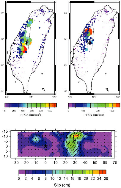
FIGURE 4.8 Peak ground acceleration (top left) and peak ground velocity (top right) of the 1999 Chi-Chi earthquake. The station coverage of the Central Weather Bureau Seismic Network is still poor in relatively inaccessible central mountainous areas. Bottom: Depth cross section showing the slip distribution derived from this data set using a finite-fault inversion methodology. SOURCE: W.-C. Chi, D. Dreger, and A. Kaverina, Finite source modeling of the 1999 Taiwan (Chi-Chi) earthquake derived from a dense strong motion network, Bull. Seis. Soc. Am., 91, 1144-1157, 2001. Copyright Seismological Society of America.
source parameters of aftershocks and their relationships to the main shocks—important data for studies of rupture propagation, postseismic relaxation, and stress transfer. Recordings of aftershocks have also begun to elucidate the causes of anomalous ground shaking and damage concentration, including basin resonance, basin-edge effects, and Moho reflection (see Section 3.1). Various forms of telemetry are making it possible to monitor state of health and to retrieve ground-motion data in near real time, allowing portable arrays to be integrated with permanent seismic monitoring systems for a wide range of seismic applications.
Imaging the Earth
Investigations of Earth structure have always figured prominently in the study of earthquakes because they frame the interpretation of seismograms in terms of source processes. Indeed, the problems of discovering the space-time structure of faulting and the three-dimensional variations in the Earth’s elastic properties are strongly coupled and must be worked out together, either through joint inversion of the seismograms or iteratively through successive approximations. The primary seismological parameters needed to specify Earth structure are the local speeds of the two basic types of seismic waves, compressional (vp) and shear (vs), their associated attenuation factors, and the mass density (27). The variations in Earth structure that can be resolved are limited by the size and spacing of the seismic array and the distribution of seismic sources used to illuminate the array. Global networks can therefore determine worldwide structure at relatively low spatial resolution (Figure 4.4), whereas regional and local networks give finer details but only within more limited volumes of the Earth (Figure 4.9).
Portable arrays are useful in enhancing the structural resolution at spatial scales below the station spacing of permanent arrays. They can be deployed in two basic modes of observation: (1) to record artificial sources—explosions, mobile ground-shaking devices such as Vibroseis, or marine air guns—by high-frequency sensors (active-source experiments) and (2) to record signals from natural events, either regional or teleseismic earthquakes (passive experiments). PASSCAL experiments use both modes. Shallow structure (in the upper 2000 meters) can be imaged with highly portable, multichannel systems that record waves reflected from subsurface discontinuities, using hammer blows or small charges as sources. For example, in the Los Angeles Region Seismic Experiment (LARSE), researchers used air guns and explosions to construct images of the subsurface structure that may lead to a better understanding of earthquake hazards in southern California (Figure 4.10). These systems have proved very effective in delineating fault planes within sedimentary ba-
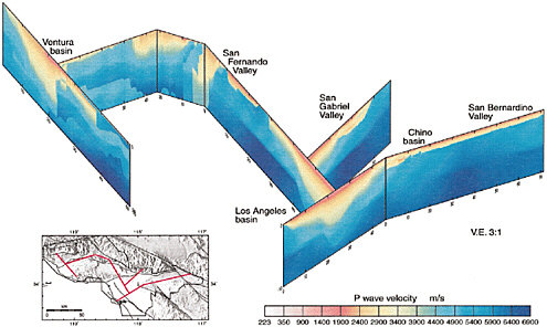
FIGURE 4.9 Fence diagram showing three-dimensional variation of shear-wave speeds in the Los Angeles region determined from seismic tomography. Cross sections are located as red lines in the lower left panel. Low speeds indicated by warm colors show deep sedimentary basins that trap seismic waves, thus amplifying and extending the shaking in regional earthquakes. SOURCE: H. Magistrale, S. Day, R.W. Clayton, and R. Graves, The SCEC southern California reference three-dimensional seismic velocity model version 2, Bull. Seis. Soc. Am., 90, S65-S76, 2000. Copyright Seismological Society of America.
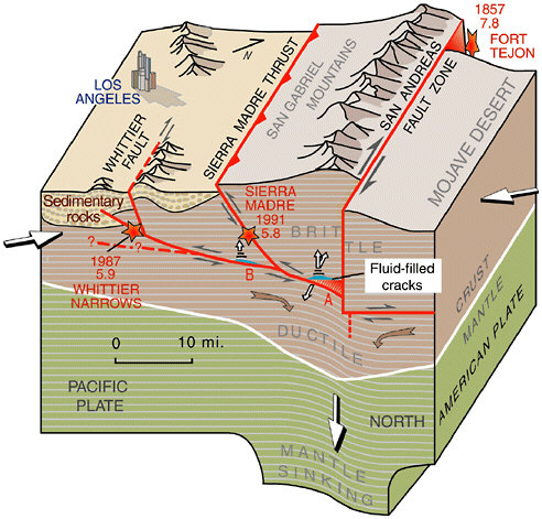
FIGURE 4.10 An interpretation of the geologic structure along Line 1 of the Los Angeles Region Seismic Experiment line, showing the interaction of strike-slip and thrust faults. “Blind” thrust faults, such as the one responsible for the 1987 Whittier Narrows earthquake, do not break the surface, but can be imaged by seismic methods. Relative movement on faults is shown by pairs of small arrows. Large white arrows show the olique direction in which the Pacific Plate (left) and the North American Plate (right) are converging. Red stars with dates and numbers (magnitudes) are earthquakes. SOURCE: U.S. Geological Survey, Fact Sheet 110-99, <http://geopubs.wr.usgs.gov/fact-sheet/fs110-99/>.
sins. Deep structure (down to the base of the crust at 30- to 40-kilometer depth) can be imaged using larger multichannel systems in conjunction with explosion or large Vibroseis sources.
Seismicity Catalogs
The basic product of seismic monitoring is the seismicity catalog, a sequential listing of all earthquakes, explosions, and other localized seismic disturbances, natural or man-made. In modern monitoring systems, the detection, association, and inversion of seismic arrivals are done automatically from continuous digital data streams, although seismic analysts are still employed to review, evaluate, and often modify the results. The output may include the event’s origin time, hypocentral location (latitude, longitude, and depth), magnitude, and other source parameters, such as seismic moment and focal mechanism (usually in the form of a moment tensor) and a measure of rupture duration. Improving the completeness and accuracy of these seismicity catalogs is a major objective of seismic hazard analysis, which often depends on small earthquakes to identify the potential for damaging fault ruptures, and of earthquake physics, which relies on catalogs as the basic space-time record of fault-system behavior.
The USGS National Earthquake Information Service (NEIS) operates an Earthquake Early Alerting Service to determine as rapidly as possible the location and magnitude of significant earthquakes in the United States (M = 4.5) and around the world (M = 6.5, or known to be damaging) (28). The International Seismological Centre (ISC), based at Thatcham in Berkshire, United Kingdom, is a nongovernmental organization charged with producing a standard global catalog (29); it provides the most comprehensive compilations of short-period arrival times and amplitudes from the largest, most globally distributed set of seismic stations (approximately 3000), including earthquake reports from a number of regional seismic monitoring agencies. It currently processes about 5000 events per month worldwide. The International Monitoring System (IMS) currently operates 36 primary stations and arrays and collects data from 38 auxiliary stations. It produces an earthquake bulletin, the Reviewed Event Bulletin, within seven days, aiming at completeness down to M 3.5 (see Box 4.2). Specialized catalog services are rendered by university observatories and laboratories. Harvard University produces a global catalog of centroid locations, centroid times, and moment tensors for most large earthquakes (M = 5.5), primarily from the broadband data provided by FSDN stations (30). Though operated on a very modest budget through a private university, this centroid-moment tensor service has proven to be immensely useful in earthquake research, be-
|
BOX 4.2 Nuclear Monitoring Since the first underground nuclear tests in the late 1950s, underground test monitoring and test ban treaty verification have motivated the development of better seismic networks (see Section 2.3). With the breakup of the former Soviet Union and the increased number of emerging nuclear nations, the emphasis has shifted from a bilateral superpower test ban treaty to a global comprehensive test ban treaty (CTBT) and the Nuclear Nonproliferation Treaty. In the current plans, seismic networks represent one of four main technologies for monitoring the CTBT (along with infrasonic, hydroacoustic, and radionuclide techniques). The seismic component of the IMS will utilize 170 stations and reduce the global detection threshold to around mb4.0. The primary stations (alpha stations) are mostly dense arrays of high-quality, short-period sensors, located at carefully selected sites around the globe, with equipment for continuous telemetry to the International Data Center (IDC) for the primary purpose of detecting seismic events on a global scale. Auxiliary stations (beta stations) are meant to support rapid, on-demand, automatic retrieval of data for use in improving the location of events detected by the primary network. Most of the beta stations will be drawn from established three-component, broadband stations of the FDSN, ensuring a strong partnership between the CTBT monitoring community and earthquake scientists. Approximately 1000 separate channels of seismic data will be transmitted via satellite in real time to the IDC in Vienna, Austria, where they will be analyzed automatically to determine routine source parameters such as location, depth, origin time, and magnitude. Although the ultimate capabilities of the monitoring system will not be known until the network is fully deployed and operational, the experience with recent nuclear tests in India and Pakistan suggests that the IDC and IMS will provide an unprecedented system for real-time global seismic monitoring with low detection thresholds.1 Monitoring CTBT compliance will be more challenging than past arms control treaties, because it will require high-confidence identification of any nuclear explosion, however small, carried out in remote regions of the world. The CTBT has motivated a broad program of research, focused on regional monitoring of small seismic events.2 The results of this research are needed for two treaty monitoring goals. First, there is a need to locate all of the detected seismic events within 1000 square kilometers, because this is the largest region that can be inspected to assess a possible treaty violation. Achieving this goal will require detailed seismic calibration information (travel times, phase arrivals) for each of the IMS stations. Second, algorithms must screen out the large number of natural events that will be detected, based on location, depth, and other source characteristics. To advance these capabilities, the Department of Defense (DOD) currently supports one of the largest basic research programs in seismology in the federal government ($12 million in FY 2000). To increase the involvement of earthquake researchers, DOD plans to make all of the IMS data available for open research and hazard monitoring operations. |
cause it has generated the longest catalog of standardized source parameters—seismic moment, source mechanism, and centroid location— for seismicity studies worldwide.
Currently, the properties of more than 30,000 earthquakes are recorded, studied, and cataloged on an annual basis by these and other monitoring organizations. A few regional monitoring systems routinely catalog all seismicity above M 2. Broadband regional networks routinely produce moment tensor solutions for regional earthquakes greater than M 4 (e.g., Figure 4.11). In many regions, however, sensor arrays are too sparse to record events below about M 3. Further work is needed to upgrade regional networks to broadband instrumentation and digital telemetry, a task taken on by the ANSS program, and to extend cataloging procedures to include additional source parameters such as characteristic dimensions (31).
Volcano Seismology
Earthquake seismology plays an important role in the study of volcanoes and the prediction of volcanic eruptions (Box 4.3). Seismicity within a volcano is caused by rockfalls and avalanches, tectonic faulting, rock fracture during magma transport, and low-frequency tremors associated with the flow of melt below a volcano. Before a major eruption, earthquakes typically occur in swarms, where the rates of seismicity may be elevated by two to three orders of magnitude above background levels. Monitoring of this activity by seismic networks yields information about the shape, size, and physical state of magma reservoirs (32). A complete understanding of the volcanic system will require a synthesis of seismological observations into a coherent model of eruption mechanics, constrained by fluid dynamics and elastodynamics of magma flow in a porous, brittle media. Recent advances in portable instrumentation and theory for analyzing the data are stimulating important advances in this field. For example, results obtained at Redoubt volcano using nonlinear, travel-time tomography show that imaging the three-dimensional structure of a volcano is feasible down to a scale of a few hundred meters (33).
Beyond first-order mapping of the fluid-pathway geometry using broadband data there are many questions about the dynamics of magma transport that can be investigated using short-period seismic data. For example, two basic families of volcanic processes generate signals in the 0.1- to 1-second seismic band. The first involves volumetric sources in which the fluid plays an active role in the generation of elastic waves, and the second consists of shear or tensile sources caused by brittle rock failure. In volumetric sources, elastic radiation is generated by multiphase fluid flow through cracks and conduits; long-period events, volcanic
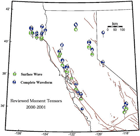
FIGURE 4.11 Moment tensor solutions for northern California obtained from the Berkeley Digital Seismic Network, illustrating advanced processing for regional earthquakes. These solutions are obtained automatically and in quasi-real time using broadband data for a subset of events of M 4 and larger. Robustness of the solution is assessed by comparing the results of two independent inversions— one in the time domain, the other in the frequency domain. SOURCE: B. Romanowicz, D. Dreger, and H. Tkalcic, University of California, Berkeley.
tremor, and seismic signals related to mechanisms of degassing in open vents are manifestations of such processes. The second family includes volcano-tectonic earthquakes, in which magmatic processes provide the source of energy for rock failure. These sources occur in the brittle rock around a magma reservoir and conduit and are associated primarily with the structural response of the volcanic edifice to the intrusion and/or
|
BOX 4.3 Prediction of the Mt. Pinatubo Eruption Mt. Pinatubo in the Philippines is one of a chain of composite volcanoes known as the Luzon volcanic arc, which are being formed by the rise of magma from an eastward-dipping subduction zone along the Manila Trench. On the afternoon of April 2, 1991, villagers were surprised by a series of small explosions from a line of vents near the north flank of the summit dome. Within a few days, scientists from the Philippine Institute of Volcanology and Seismology (PHIVOLCS) installed several portable seismographs near the northwest foot of Mt. Pinatubo and began recording small earthquakes at a rate of about 40 to 140 per day. In late April, PHIVOLCS was joined by a group from the USGS, and the joint team installed a network of seven seismometers, telemetered to Clark Air Base, a major U.S. Air Force facility located just east of the volcano. Numerous small earthquakes (M lower than 2.5) continued through May, clustered in a zone 2 to 6 kilometers deep and caused by fracturing of brittle rock by rising magma. Beginning on June 1, a second cluster of earthquakes developed in the upper 5 kilometers near the fuming summit vents. A small explosion early on June 3 initiated an episode of increasing volcanic unrest characterized by intermittent minor emission of ash, increasing seismicity beneath the vents, and episodes of harmonic tremor (a prolonged rhythmic seismic signal believed to be related to sustained subsurface movement of magma or volatile material). PHIVOLCS issued a level-3 alert on June 5, indicating the possibility of a major pyroclastic eruption within two weeks. A tiltmeter high on Mt. Pinatubo began to show a gradually increasing outward tilt early on June 6. Seismicity and the outward tilt continued to increase until late afternoon on June 7, when an explosion generated a column of steam and ash 7 to 8 kilometers high. After the explosion, seismicity decreased and the increase in outward tilt stopped. PHIVOLCS promptly announced an increase to level-4 alert (eruption possible within 24 hours) and recommended additional evacuations from the volcano’s flanks. The period from June 8 through early June 12 was marked by continuing, weak ash emission and episodic harmonic tremor. On June 9, PHIVOLCS raised the alert level to 5 (eruption in progress). The radius of evacuation was extended to 20 kilometers, and the number of evacuees increased to about 25,000. The first major explosive eruption began at 0851 hours on June 12, generating a column of ash and steam that rose to 19 kilometers. Although a burst of seismic tremor had occurred several hours earlier, no specific seismic precursor immediately preceded this event; a high-amplitude seismic signal and the rise of the eruptive column seemed to begin simultaneously. Seismic records indicated that this event lasted about 35 minutes. This was the first of a series of brief explosive eruptions that occurred with increasing frequency from June 12 through 15. The climactic eruption began at 1430 hours on June 15—the world’s largest in more than half a century. The successful forecast of the Mt. Pinatubo eruption enabled Philippine civil leaders to organize massive evacuations that saved thousands of lives and greatly reduced the destruction at Clark Air Base (military aircraft worth $200 million to $275 million were also removed).1 Nevertheless, the coincidence of the climactic eruption with a typhoon led to more than 300 deaths and extensive property damage, caused primarily by the extraordinarily broad distribution of heavy, water-saturated tephra-fall deposits. |
withdrawal of fluids. Volcano-tectonic earthquakes act as stress gauges that map stress concentrations in the volcanic structure. Dense distributions of earthquake hypocenters therefore provide a signature of magma migration through volcanoes. However, gaining a better understanding of the dynamics of magma transport will require more information about the source processes for the long-period events (34).
4.2 TECTONIC GEODESY
The elastic strain energy unleashed in earthquakes accumulates in the Earth’s crust through the imperceptibly slow motions of plate tectonics. The strain rates in tectonically active areas such as the western United States are only few parts in 10 million per year (35). The tools of geodesy can be used to measure these small tectonic deformations on global to local scales, furnishing data that have proven essential for estimating the long-term slip rates and seismogenic potential of lithospheric faults. In addition, geodesy provides the means to detect transient (time-localized) strains having durations from minutes to years that do not generate elastic waves and are therefore invisible to seismic monitoring. These transients comprise fault creep and stress relaxation following large earthquakes (postseismic transients), as well as the slow, localized strains that are predicted by laboratory experiments to precede dynamic faulting (deformation precursors). They also include an observed but poorly understood class of isolated events known as “silent earthquakes,” which may be responsible for aseismic slip on some faults and may play a role in concentrating stress before some large earthquakes.
Tectonic geodesy includes a wide array of techniques with complementary strengths and sensitivities. Geodetic measurements vary in scale from systems that allow the recovery of three-dimensional position anywhere on the planet’s surface, such as GPS, to systems that are extremely localized and sensitive, such as borehole strainmeters.
Traditional Geodetic Techniques
Many of the measurement technologies used in tectonic geodesy grew out of the needs of precise surveying. Both activities share a requirement for extremely precise measurements, and the practice of geodesy has a strong tradition of characterizing and minimizing measurement errors.
-
Triangulation. This surveying technique, invented by ancient agricultural societies, can measure angles between distant points with a precision of approximately 2 arc-seconds, corresponding to a shear strain of about 5 parts per million. Triangulation requires a clear line of sight from
-
an observing station to two or more target monuments, typically a few tens of kilometers distant (usually situated on high ground). Triangulation played an important role in estimating the strains and displacements associated with the 1906 San Francisco earthquake, providing much of the observational foundation for Reid’s elastic rebound model. Triangulation is expensive, however, because observing and target sites must be occupied simultaneously by experienced personnel. Consequently, the method has been largely abandoned by the tectonic geodesy community in favor of more accurate and flexible techniques, primarily GPS (described below).
-
Trilateration. In the 1970s, the ability to measure long distances with laser reflectors improved the utility of tectonic geodesy. Trilateration provided the means for repeated strain measurements over baselines of tens of kilometers with sufficient precision (about 300 parts per billion) to monitor the strain accumulation between large earthquakes (36). It allowed the USGS to confirm that slip rates observed over decades across major faults in California are quite similar to geological estimates, which are averaged over thousands to millions of years. Like triangulation, this method has been superceded by GPS.
-
Spirit Leveling. Vertical displacements measured by spirit leveling have been used to characterize the vertical component of the deformation field associated with earthquakes (37). Reports of postseismic and even precursory deformation measured with leveling have been published, but the limited accuracy and the possibility of systematic error have made these reports controversial (38). Leveling surveys are very labor intensive and costly, although they remain the most precise way to measure relative elevations over distances of less than about 25 kilometers. Over larger distances, GPS provides a more accurate, and much more economical, alternative to leveling (39) and offers the tremendous advantage of continuous temporal sampling.
Space Geodetic Systems
The space program has contributed much of the new technology developed for tectonic geodesy since the 1970s. Ultraprecise methods of space-based geodesy were first pioneered in Very Long Baseline Interferometry using astronomical sources, but they reached their current state of capability by taking advantage of dedicated satellite platforms.
-
Very Long Baseline Interferometry (VLBI) and Satellite Laser Ranging (SLR). The pioneering geodetic techniques of VLBI and SLR, both capable of monitoring plate motions at a global scale, were developed under the National Aeronautics and Space Administration (NASA)
-
Crustal Dynamics Program. VLBI uses simultaneous observations of high-frequency radio waves from extragalactic quasars to measure the baselines connecting a set of radio telescopes. Precision approaches one part per billion—millimeter changes over 1000-kilometer baselines. SLR uses laser pulses reflected from special satellites (e.g., Laser Geodynamics Satellite and Starlette) to locate optical telescopes on the ground. SLR is less precise than VLBI because of lower signal-to-noise levels and the need to solve for the motion of the satellite and ground stations. VLBI confirmed Wegener’s concept of continental drift and provided a rough approximation of how the Pacific-North American plate motion is distributed across western North America (40). SLR also contributed data to the study of plate boundary deformation zones, particularly in the Mediterranean region. VLBI and SLR are both very cumbersome and expensive because they require sensitive instrumentation to detect very weak signals. Consequently, they have been replaced in nearly all tectonic applications with GPS measurements.
-
Global Positioning System. Tectonic geodesy was rapidly transformed by the deployment of the first GPS constellation in the mid-1980s. These satellites emit strong, precisely timed radio signals easily detectable by 100-millimeter antennae and can be used to locate points anywhere on the Earth’s surface. GPS instrumentation, which underlies most modern autonomous satellite navigation systems and a host of military and commercial applications, has become quite affordable since its initial development, so GPS surveying can be done by individual investigators (41). Because of its low cost and portability, GPS has quickly replaced other geodetic techniques for most tectonic studies, including dense sets of deformation measurements spanning plate boundaries (42).
GPS locations are measured relative to the orbiting satellites, whose positions are in turn estimated relative to tracking stations on the ground. Geodetic accuracy thus depends on knowing the location of the tracking stations, which are moving relative to each other because of tectonic motions. At present, the tracking station coordinates are best determined by making frequent GPS measurements at sites tied into a standard (absolute) reference frame by VLBI or SLR observations (43).
GPS measurements can be performed in either campaign or permanent modes. The campaign mode involves temporary occupation of geodetic benchmarks in much the same way as for earlier triangulation and trilateration surveys. A series of issues—the decreasing costs of receivers, the high labor costs of campaign measurements, the loss of precision caused by antenna setup—has motivated the installation of permanent GPS stations in configurations similar to seismic monitoring networks. Automated arrays of continuously sampled GPS receivers can measure deformation in real time as often as once per minute (44). Japan has the
largest fixed GPS network with more than 1000 stations. In comparison, the Bay Area Regional Deformation network in northern California includes about 35 stations and the Southern California Integrated GPS Network (SCIGN) now comprises 250 stations (Figure 4.12). The arrays in Japan and southern California have tested many design elements and demonstrated what features of time-dependent strain are most significant. Permanent GPS arrays will continue to grow as receiver and data-transmission costs drop further.
Plans call for the permanent GPS networks in the western United States to be expanded and consolidated to form a major component of the Plate Boundary Observatory (PBO), proposed as part of the EarthScope program (see Chapter 6). The GPS component of the PBO would comprise more than 1000 continuously recording GPS receivers, with several hun-
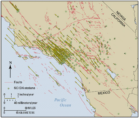
FIGURE 4.12 Velocities relative to the North American Plate of geodetic movements from 15 years of GPS measurement in Southern California, showing ongoing deformation within a complex system of faults. SOURCE: Southern California Earthquake Center and U.S. Geological Survey.
dred established as a geodetic backbone for the study of plate boundary tectonics. The remaining GPS stations would be deployed in denser clusters to provide detailed data on active faults and volcanic systems within the most active zones.
The broad coverage and high precision of GPS geodesy permit individual faults to be studied as components in strongly interacting systems rather than as isolated elements. A disadvantage of GPS is that motion can be measured only at points on the ground where receivers are located. Although the cost of GPS receivers is decreasing steadily, it is impossible to measure the deformation field densely enough to answer some key questions of earthquake science.
-
Interferometric Synthetic Aperture Radar. The most recent innovation in tectonic geodesy is InSAR, which has imaged earthquake deformations at a level of detail unanticipated only 10 years ago (45). InSAR measures deformation by comparing reflected radar waves recorded on successive passes of a satellite from nearly identical positions. The simplest InSAR measurements are sensitive to just one component of displacement (toward the satellite), but stereoscopic measurements (pairs of images from multiple locations) allow measurement of vector displacements (Figure 4.13). InSAR is subject to errors from changes in reflective properties such as those caused by seasonal vegetation changes and snowfall, and it lacks the temporal resolution of GPS. However, the ability to map essentially continuous displacements over large swaths of active plate boundaries offers an enormous advantage.
Because they can map centimeter-level deformations with a spatial resolution on the order of 100 meters, InSAR systems are useful for determining co-seismic and interseismic slip on faults. This is particularly important in remote areas lacking GPS stations. InSAR has shown an ability to measure co-seismic slip on subsidiary faults, variations in slip distribution along strike, and slip on previously unknown faults. With its continuous coverage, InSAR systems can map surface displacements before, during, and after earthquakes or volcanic eruptions, providing time-dependent data on the mechanics of fault loading, earthquake rupture, and earthquake interaction, and they can image strain accumulation across broad tectonic zones (Figure 4.14), as well as regional subsidence induced by petroleum production and groundwater withdrawal. For example, InSAR data have been used to disentangle the latter types of motion from tectonic strains observed by GPS networks in the Los Angeles basin (Figure 4.15). Finally, InSAR has been used to detect postseismic poroelastic effects induced by fault movements (46). An important component of the proposed EarthScope project is a dedicated InSAR satellite, the Earth Change and Hazard Observatory (ECHO) (47).
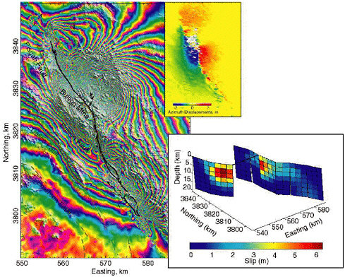
FIGURE 4.13 InSAR-derived interferogram (left) and azimuth offset field (upper right) show the surface deformation from the October 20, 1999, M 7.1 Hector Mine earthquake as determined by M. Simons et al. (2002). Colored fringes show radar phase introduced by earthquake-induced changes in distance from each point on the ground to the orbiting radar. A solution for fault slip at depth inferred from the radar data (lower right) as determined by Jonsson et al. (2002) indicates a maximum slip of 6 meters at 10-kilometer depth just northwest of the hypocenter. The fault has two branches in its northern part: the westernmost branch, which has greater slip than the eastern branch, has been offset in the figure for clarity. SOURCE: M. Simons, Y. Falko, and L. Rivera, Coseismic deformation from the 1999 Mw 7.1 Hector Mine, California, earthquake as inferred from InSAR and GPS observations, Bull. Seis. Soc. Am., 92, 1390-1402, 2002; S. Jonsson, H. Zebker, P. Segall, and F. Amelung, Fault slip distribution of the Mw 7.1 Hector Mine, California, earthquake estimated from satellite radar and GPS measurements, Bull. Seis. Soc. Am., 92, 1377-1389, 2002. Copyright Seismological Society of America.
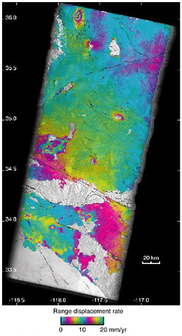
FIGURE 4.14 InSAR-observed deformation along the San Andreas fault from European Remote Sensing satellite radar. Many interferograms were combined to detect the elastic strain built up along the fault during the interval from 1992 to 2000. One color cycle shows 10 millimeters per year of ground displacement. Other local deformation signatures due to groundwater and oil withdrawal in urban areas are clearly visible. InSAR also reveals unexpected transient strain accumulation along the Blackwater-Little Lake fault system within the eastern California shear zone in a 120-kilometer-long, 20-kilometer-wide zone of concentrated shear between the southern end of the 1872 Owens Valley earthquake surface break and the northern end of the 1992 Landers earthquake surface break. The shear zone is continuous through the Garlock fault, which does not show any evidence of left-lateral slip during the same period. A dislocation model of the observed shear indicates right-lateral slip at 7 ± 3 millimeters per year on a vertical fault below 5 kilometers depth, a rate that is two to three times greater than the geologic rates estimated on northwest-trending faults in the eastern Mojave area. SOURCE: G. Peltzer, F. Cramp, S. Hensley, and P. Rosen, Transient strain accumulation and fault interaction in the eastern California shear zone, Geology, 29, 975-978, 2001.
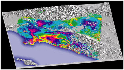
FIGURE 4.15 Perspective view of the Los Angeles region with superimposed InSAR measurements of ground motions between May and September 1999, indicating seasonal and secular variations due to groundwater withdrawal and recharge. Large regions of metropolitan Los Angeles are rising and falling by up to 11 centimeters annually, and a large portion of the city of Santa Ana is sinking at a rate of 12 millimeters per year. The repeated color banding with the large oval shows approximately 5 centimeters of subsidence. The straight line located just inside the coastline is the Newport-Inglewood fault, which controls the extent of subsidence. The small isolated bull’s-eye feature north of Palos Verdes and east of downtown Los Angeles is from pumping activity in the Inglewood oil field. The motion caused by the withdrawal of water, oil, and gas from the basin contaminates GPS measurements of the deformation field. After corrections for these effects using the InSAR data, the contraction across the Los Angeles Basin is estimated to be approximately 4.5 millimeters per year. This deformation is thought to be accommodated primarily on blind thrust faults, such as those that ruptured in the 1987 Whittier Narrows and 1994 Northridge earthquakes. SOURCE: G.W. Bawden, W. Thatcher, R.S. Stein, K.W. Hudnut, and G. Peltzer, Tectonic contraction across Los Angeles after removal of groundwater pumping effects, Nature,412, 812-815, 2001. Reprinted by permission from Nature copyright 2001 Macmillan Publishers Ltd.
Strain Measurements
A separate facet of geodesy is the measurement of strain over small spatial scales using self-contained instruments called strainmeters. The discovery in 1960 of aseismic slip or “creep” on a segment of the San Andreas fault in central California (48) led to methods for extremely localized measurements of fault displacement using invar tapes, wire creep-
meters, alignment arrays, short-baseline triangulation, and laser length surveys (49). Deployment of these instruments revealed both steady and episodic creep occurring at shallow depths (<4 kilometers) on some faults, often near the time of earthquakes (50). Aseismic creep at greater (seismogenic) depths, such as observed in central California, appears to be rare.
High-resolution laser strainmeters, borehole strainmeters, and tiltmeters are used to measure deformation very precisely in a small region. Their sensitivity approaches 10–12, but long-term stability is a problem because they have small footprints susceptible to very localized, nontectonic deformations, such as ground swelling in rainstorms. The most stable instruments are the laser strainmeters and water-tube tiltmeters at Piñon Flat Observatory in California, which derive their stability from their length (>500 meters) and the “optical anchors” used to couple the end monuments to rock at about 25-meter depth (51). Borehole instruments suffer drift over several months, but they are very precise over shorter times and have widespread application for measuring transient deformation, including slow and silent earthquakes (52).
Under the best conditions, these instruments are as much as two to three orders of magnitude more sensitive than GPS at short periods. At longer periods, the relative advantage declines significantly, although long-baseline instruments may retain advantages even for time scales of years. Because they measure strain, which decays as the cube of distance from a dislocation, they must be positioned in reasonably close proximity to the source. Small numbers of borehole strainmeters have been operating for years in a few select locations. The proposed Plate Boundary Observatory would deploy several hundred borehole and perhaps several long-baseline strainmeters at strategically chosen sites along the San Andreas fault system, as well as at several volcanic systems (53).
Geodetic Observations of Earthquake Processes
The increasing precision and density of geodetic measurements are furnishing new constraints on how complex fault systems are loaded, how earthquakes interact, the nature of aseismic deformation transients, and how the rheological structure of the Earth’s crust controls the earthquake process.
Plate Tectonics and Fault Motions Geodetic studies have shown that plate-tectonic models, based on data that average over thousands to millions of years, can accurately predict the short-term motions across plate boundary zones a few hundred kilometers wide. Denser measurements from geodetic networks place strong constraints on the slip rates
on faults within these zones and are especially valuable for faults that are poorly exposed or otherwise not amenable to geological study. If proper accounting is made for fault interactions and postseismic deformations, geodetic slip rates for faults bounding small tectonic blocks with lateral dimensions of 20-50 kilometers generally agree with those estimated by geologic methods for much longer time intervals, although clear discrepancies have been documented (Figure 4.14).
By integrating the slip rate over the areas of faults, one can estimate the rate at which seismic moment is accumulating. If it can be assumed
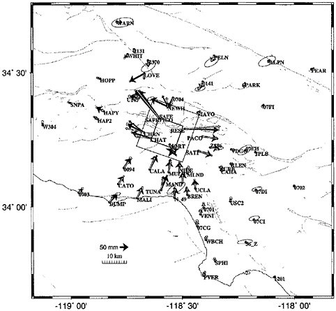
FIGURE 4.16 Horizontal displacement (heavy black vectors and the corresponding one-sigma error ellipses) associated with the Northridge earthquake measured by the GPS network in southern California. SOURCE: K.W. Hudnut, Z. Shen, M. Murray, S. McClusky, R. King, T. Herring, B. Hager, Y. Feng, A. Donnellan, and Y. Bock, Coseismic displacements of the 1994 Northridge, Calif., earthquake, Bull. Seis. Soc. Am.,86, S19-S36, 1996. Copyright Seismological Society of America.
that all of this moment is released in earthquakes (no aseismic slip) and if the relative distribution of earthquake size is known, then the long-term moment rate sets the multiplicative constant needed to infer long-term earthquake frequency (54). Because aseismic creep at seismogenic depths seems to account for very little of the moment budget in most continental settings, unknown fault geometry and uncertainties in the earthquake size distribution are often the limiting factors in estimating earthquake frequency (55).
Strain rates depend on the slip distribution and geometry of faults, so spatial variations in measured strain rate reveal significant information about the faults. For example, spatial variations of strain rate along the San Andreas fault near Parkfield, California, show details of the slip rate on the fault plane. The San Andreas is primarily locked to a depth of about 15 kilometers to the southeast of that location and is creeping to the northwest. The slip distribution is important for understanding the physical mechanism of the transition and the stress accumulation leading to future earthquakes (56).
The crust on either side of the creeping section of the San Andreas fault accumulates very little strain, and the geodetic displacement rate (35 millimeters per year) is virtually identical to the geologic slip rate on the San Andreas (34 millimeters per year). Elsewhere on the San Andreas and on other strike-slip faults, secular deformation is continuous across each fault. The deformation patterns can be matched with a model in which each fault is locked by friction to a depth of 10 to 20 kilometers and slips freely below that depth in a viscoelastic lower crust.
Earthquake Rupture and Subseismic Strain Events GPS data provide independent estimates of earthquake-induced fault displacement (57), as illustrated in Figure 4.16. Geodetically derived images of slip variations for the recent Loma Prieta and Landers earthquakes rival the spatial resolution achieved from models based on seismic data (58). In the case of the 1989 Loma Prieta earthquake, a geodetically derived slip model (59) supported seismic models that found a variation of slip direction with distance along the fault (60). Models of the 1992 Landers, California, earthquake based on GPS data confirm the strong spatial variability and location of slip derived from modeling the strong motion data (61).
The 1992 Landers, 1999 Izmit (Turkey), and 1999 Hector Mine earthquake all caused substantial deformation not detectable with existing GPS arrays. InSAR images from the Landers earthquake show co-seismic slip on the Garlock and other faults, which were not otherwise known to have slipped in the main shock (62). Many subsidiary faults, some previously unmapped, slipped more than 10 millimeters during the 1999 Hector Mine earthquake.
Geodetic data for the 1989 Loma Prieta and 1994 Northridge earthquakes reveal co-seismic deformation that cannot be explained by slip on the seismically determined fault plane. This deformation may have been caused by vertical variations in elastic moduli or by secondary deformation in the hanging wall of these faults (63).
One of the most significant discoveries in tectonic geodesy has been the detection of episodic strain transients that have earthquake-like spatial patterns but occur too slowly (over days to months) to excite seismic waves. These subseismic events, or “silent earthquakes,” have been observed in volcanic areas, such as the M 7 Izu-Oshima earthquake in 1978 (64), and on shallow creeping faults such as the San Andreas between Parkfield and San Juan Bautista (Figure 4.17). Continuously recording stations of the Japanese GPS network detected a much larger event (M 6.5) with a duration of about a year on the subduction interface under the Bungo Channel, between the islands of Shikoku and southern Honshu (Figure 4.18). In 1999, a Canadian team used GPS networks in southwest British Columbia and northwest Washington to detect a 15-day, M 6.7 silent slip event at depths of 30-40 kilometers on the Cascadia subduction interface (65). Further analysis of a full decade of continuously recorded data has uncovered a quasi-periodic series of similar events with an average recurrence interval of about 14 months (66). It is not yet known whether such sequences are characteristic of subduction zones, nor is it understood how these subseismic transients relate in time and space to great earthquakes that occur every several hundred years along shallower segments of the subduction interface. These research problems have clear connections to the fundamental issues of earthquake predictability.
PostSeismic Deformation and Long-Term Transients The stress changes from large earthquakes cause several types of secondary deformation that can be detected by surface geodesy. These include additional slip on the fault surface (afterslip); viscous relaxation in the hotter, more ductile lower crust; and pressure-driven fluid flow. Postseismic strain transients due to one or more of these mechanisms have been documented for a number of earthquakes, such as 1906 San Francisco (67), 1957 Kern County (68), 1985 Central Chile (69), and 1989 Loma Prieta (70). The 1992 Landers earthquake, where the cumulative postseismic deformation may have equaled 10 to 20 percent of the M 7.3 mainshock, was the first to be observed by a full suite of modern geodetic methods: GPS (71), laser strainmeters (72), and InSAR (73). The strain transients observed by these techniques had different durations—about 6, 50, and 1000 days, respectively—either because of different instrumental sensitivities or because separate inelastic processes were operating (Figure 4.19). More recent
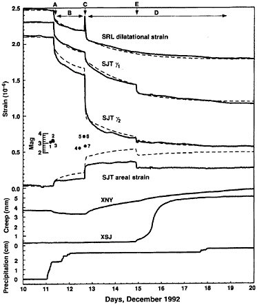
FIGURE 4.17 Borehole strain and creepmeter data from San Juan Bautista for 10 days in December 1992, showing several slow earthquakes. The observations suggests rupture speeds of 0.1 to 0.5 meter per second for these events, compared to 1 to 5 kilometers per second for ordinary earthquakes. SOURCE: A.T. Linde, M.T. Gladwin, M.J.S. Johnston, R.L. Gwyther, and R.G. Bilham, A slow earthquake sequence on the San Andreas fault, Nature, 383, 65-68, 1996. Reprinted by permission from Nature. Copyright 1996 Macmillan Publishers Ltd.
earthquakes, including the 1999 Izmit and 1999 Hector Mine events, have added data sets of similar diversity that are under active analysis.
Viscoelastic diffusion following large earthquakes in California and Japan generates large strain changes, even decades later. Several authors have argued that the resulting stresses might propagate slowly, contributing to deformation and possibly earthquake triggering at very great distances from a large earthquake (74).
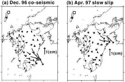
FIGURE 4.18 Observations of slow earthquake under the Bungo channel between Kyushu and Shikoku observed by the continuously recording Japanese GPS network. The GPS-derived vector motions indicated by arrows are from (a) an ordinary earthquake on the subduction interface and (b) a subsequent silent earthquake that did not radiate seismic waves. The patterns of deformation are quite similar (though displaced), indicating that the silent earthquake represents slip on a nearby patch of the subduction interface. The moment magnitude of the silent earthquake was estimated to be M 6.8. SOURCE: Modified from Y. Yagi, M. Kikuchi, and T. Sagiya, Co-seismic slip, post-seismic slip, and aftershocks associated with two large earthquakes in 1996 in Hyuga-nada, Japan, Earth Planets Space,53, 793–803, 2001.
Tectonic Deformation and Future Earthquakes Geodetic data have confirmed Reid’s hypothesis that strain accumulates in the region surrounding a fault before a major earthquake, but not his conjecture that major earthquakes can be predicted from the time required to recover the strain released in the previous event. Although the latter has not yet been fully tested owing to measurement limitations and the lack of the long-term observations, Reid’s notion of an earthquake “cycle” appears to be at odds with the observed complexity of the earthquake process and the inherent irregularity of stick-slip behavior.
Fault-friction models derived from laboratory data predict that observable aseismic slip in the nucleation zone of an earthquake might precede the seismic phase of fault rupture on time scales of minutes to days. Hope that such signals could be used to predict large earthquakes motivated many geodetic searches for aseismic strain precursors, primarily
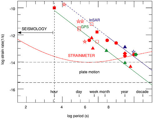
FIGURE 4.19 Thresholds of strain-rate sensitivity are shown for borehole strainmeters, GPS, and InSAR as a function of period. The diagonal lines give GPS (green) and SAR (blue) detection thresholds for 10-kilometer baselines, assuming 2-millimeter and 2-centimeter displacement resolution, respectively. GPS and InSAR strain-rate sensitivity is better at increasing periods, allowing the detection of plate motions (dashed line). Borehole strain detection threshold reaches a minimum at a period of a week and then increases with period due to Earth noise. At longer periods (months to a decade), GPS has greater sensitivity than borehole strain by one to two orders of magnitude. At intermediate periods (weeks to months) the two are comparable, and at short periods the borehole strainmeter sensitivity is one to three orders of magnitude greater. Also shown are several types of transients observed by strainmeters (red), GPS (green), and InSAR (blue). Triangles show postseismic deformation from the Landers earthquake observed by strainmeters, GPS, and InSAR. Squares show slow earthquakes; open squares show single station observations. Red and green diamonds and open circles show long-term aseismic deformation. SOURCE: PBO Steering Committee, The Plate Boundary Observatory: Creating a four-dimensional image of the deformation of western North America, White paper providing the scientific rationale and deployment strategy for a Plate Boundary Observatory based on a workshop held October 3-5, 1999. Available at <http://www.earthscope.org>.
using strainmeters and tiltmeters, which are more sensitive to short-term transients than network-based geodesy (Figure 4.19). However, no precursory strain signals have been identified reliably (75), presumably because the nucleation zones at depth are too small to cause measurable strains at the Earth’s surface.
The role of subseismic slip events in setting the stage for future earthquakes is unknown. Such events have been observed within several plate boundary fault zones (see above), but so far no convincing relationship to seismic fault slip has been demonstrated. The deformations due to subseismic events decay much more rapidly with distance from the source than seismic waves, which makes them hard to observe. Moreover, available measurement techniques leave important parts of the space-time spectrum poorly covered (Figure 4.19). Establishing the relationship between subseismic strain and future earthquakes is a clear target for research in tectonic geodesy.
4.3 EARTHQUAKE GEOLOGY
Earthquake geology was pioneered by the postearthquake investigations of Charles Darwin, G.K. Gilbert, and B. Koto in the nineteenth century. It has since evolved into three subdisciplines: neotectonics, paleoseismology, and fault-zone geology (76). The methodology and research issues comprised by the first two are the subject of this section; the third is incorporated into a following section on fault and rock mechanics.
Methods and Tools
Geologists have steadily improved their acuity in reading subtle features of the geologic record, setting the stage for the process-oriented investigations that now lead the geologic study of active fault systems. For example, earthquake geologists have collaborated with paleoclimatologists to improve understanding of the youngest part of the sedimentary record—the Holocene, comprising rocks up to about 10,000 years old—which contains substantial information about prehistoric earthquakes. At the same time, technological developments have contributed new tools for geologic exploration in both space and time.
Remote Sensing Landforms are the most readily accessible expression of active tectonics because they can be viewed remotely, for example, by space-based tonal images from System Probatoire pour l’Observation de la Terre (SPOT) or Landsat satellites (Figure 4.20). The details of land-form topography are particularly useful in measuring the rates of fault slip and associated deformations. For many years, stereopairs of aerial
photographs, in combination with topographic and geologic maps, have been primary sources of data for earthquake geologists (Figure 4.21). Digital topographic data from more precise remote-sensing platforms have been poised for some time to substantially improve the measurement and interpretation of tectonic landforms (77), but progress has been frustratingly slow. In a few wealthy countries, such as the United States or Taiwan, digital elevation models (DEMs) are available at 30- to 40-meter postings, which is fine enough to be useful for neotectonic and postseismic studies (Figure 4.22); however, the resolution across most of the world is considerably poorer (1-kilometer postings are common). NASA’s Shuttle Radar Topography Mission (SRTM) collected the first global, high-resolution topographic data set, sampling 80 percent of the land surface at 30-meter resolution (78), but national security interests have thus far prevented the release of these data.
Landforms associated with one or a few earthquakes are often so small that study requires resolution of just a few centimeters. Land-based laser-ranging “total stations” have replaced the plane table and alidade as the geologist’s means of producing detailed maps. A new technology that holds great promise for the rapid mapping of the ground surface at very high resolution is light detection and ranging (LIDAR), the laser-based equivalent of radar. LIDAR systems can be mounted on light aircraft equipped with inertial and GPS guidance systems to obtain vertical resolution at the decimeter level (79). An example of data from the 1999 Hector Mine earthquake is shown in Figure 4.23.
Methods based on the electromagnetic spectrum cannot be used to map active tectonic structures on the seafloor, where most major plate boundaries are found. Surface ships with multibeam sonar systems can map bathymetry in swaths several times as wide as the ocean depth, yielding DEMs with a resolution comparable to those currently available for much of the land surface (80). This mapping capability has thus far been focused on the ridge-transform systems of the mid-ocean spreading centers. Less detailed work has been done in oceanic trench environments and on the active continental margins (Figure 4.24). Side-scan sonar systems towed in midwater use the amplitude of acoustic reflection to image small-scale features not visible by swath mapping, such as the lineations due to faulting. Sleds of instruments towed on cables within tens of meters of the seafloor can collect bathymetric data at decimeter levels, although their deployment costs are very high and they are therefore used to survey only small regions of high interest. In shallow water, swept-frequency (“chirp”) sonar systems can penetrate shallow sediments to return detailed images of sedimentary layering and its disruption by earthquake faulting.
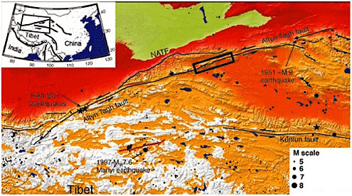
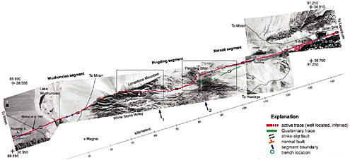
FIGURE 4.20 (top) Map of the Altn Tagh fault zone showing the regional tectonic setting and location in Asia. (bottom) Digital topography mosaic of a portion of the Altyn Tagh fault in Tibet, showing various depositional and erosional landforms that enable mapping of active faults and associated landscapes. The availability of Landsat imagery in the early 1970s allowed P.Tapponnier and P. Molnar to map the many active strike-slip faults of Tibet and surrounding regions that, at the time, were inaccessible to Western scientists. SOURCE: Z. Washburn, J.R. Arrowsmith, S.L. Forman, E. Cowgill, X.F. Wang, Y.Q. Zhang, and Z.L. Chen, Recent earthquake geology of the central Altyn Tagh fault, China, Geology,29, 1051-1054, 2001. Images are available at <http://activetectonics.la.asu.edu/atf/ATFPhotos/index.html>.
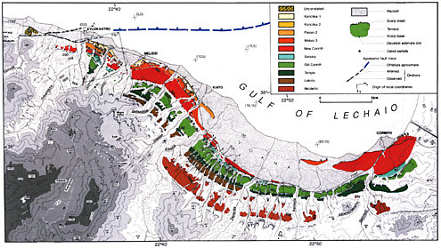
FIGURE 4.21 A flight of 10 uplifted terraces on the south flank of the Gulf of Corinth, Greece, showing progressively greater deformation with age and greater uplift toward the east. Armijo and others used these landforms to model the history and geometry of the offshore fault, as well as the response of the crust to the associated extensional deformation. SOURCE: R. Armijo, B. Meyer, G.C.P. King, A. Rigo, and D. Papanastassiou, Quaternary evolution of the Corinth Rift and its implications for the Late Cenozoic evolution of the Aegean, Geophys. J. Int.,126, 11-53, 1996. Reproduced by permission of Blackwell Publishing.
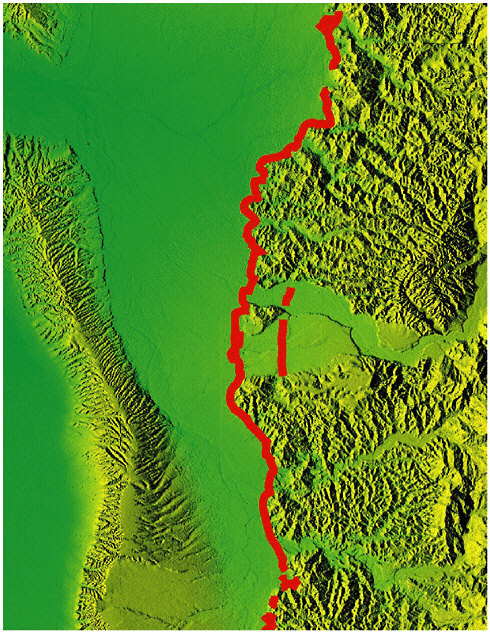
FIGURE 4.22 Shaded-relief map made from a 40-meter digital elevation model of Taiwan, used in mapping active faults and folds. Geomorphic expression of the Chelungpu fault (red line), the cause of the M 7.6 Chi-Chi earthquake in 1999, is clearly expressed. SOURCE: Charles Rubin, Central Washington University, Ellensburg, and Kerry Sieh, Caltech.
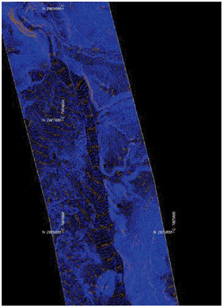
FIGURE 4.23 Topographic map of a short segment of the 1999 Hector Mine earthquake in California’s Mojave desert, constructed from LIDAR data, showing small-scale features associated with the faulting. SOURCE: K. Hudnut, U.S. Geological Survey.
Geochronology Inferring crustal deformation rates and dating events requires appropriate measures of geologic time. The dates and extent of fault ruptures can be documented by historical records (81), but only for the last couple of millennia at most. Advances in the diversity and precision of geochronological techniques are now being applied to dating the geologic layers and erosional surfaces disturbed by prehistoric earthquakes. For example, dendrochronology (the use of annual growth rings from trees) has pinned down the dates and locations of fault ruptures in Alaska and along the San Andreas fault, and has been used to determine the dates of subduction-related submergence of coastal Washington and massive seismically induced landslides in urban Seattle (82). Other dating methods used in earthquake geology include tephrochronology, thermoluminescence,
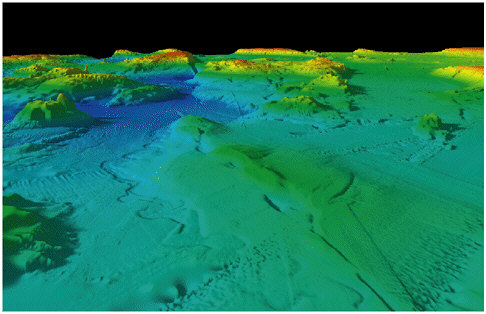
FIGURE 4.24 Three-dimensional rendering of the bathymetry offshore southern California, illustrating the quality of data now achievable from swath-mapping by surface ships. The view is toward the northwest. From center ground to lower right is the trace of the right-lateral strike-slip is San Clemente Island fault. The linear ridges have formed along a restraining bend. The red hill in the background is San Clemente Island; a spectacular fault scarp forms its eastern (right) edge. SOURCE: C. Goldfinger, Oregon State University.
optically stimulated luminescence, pedology, and lichenometry (83). The principal isotopic techniques are radiocarbon, uranium series, helium, potassium-argon, argon-argon, and fission-track dating (84).
The radiocarbon technique is the workhorse for dating sediments younger than about 50,000 years, and its application has begun to supply the time series of large earthquakes for important continental fault systems (85). The advent of accelerator mass spectrometry (AMS) has enabled the carbon dating of samples much smaller than a gram or so by conventional techniques. Radiocarbon ages can be calibrated precisely to about 10,000 years before present using dendrochronology, yielding uncertainties as small as a decade or so. The development of AMS has also been a boon to uranium-thorium disequilibrium dating. Radiocarbon and uranium-thorium analyses of replicate samples have resulted in a calibration curve for radiocarbon dates to about 30,000 years, with uncertainties of a few hundred years (86).
Uranium-thorium disequilibrium dating is gaining importance in both neotectonic and paleoseismic studies. Coral heads uplifted during paleoseismic events in Vanuatu have been dated with errors of just a few years, and similarly precise timings have been made for the uplift and submergence during large earthquakes of the Sumatran subduction zone, the long-term deformation along low-latitude coastlines, and the glacial low stands and interglacial high stands of sea level in the tropics (87). The latter provide a basis for inferring the ages of deformed coastal deposits and surfaces at high latitudes.
Knowing the age of ground surfaces can be critical to quantifying the rate of deformation of a fold, the rate of tilt of a surface, or the rate of slip across a fault, but surfaces have been notoriously difficult to date, especially beyond the 50,000-year range of radiocarbon analysis. Surface-exposure dating by cosmogenic isotopes, especially 10Be, 26Al, and 36Cl, has resolved some of these problems, and these techniques have been applied to faulting caused by the Indian-Asian collision, normal fault scarps in limestone in the eastern Mediterranean, and California marine terraces (88). The last were revealed to be tens of thousands of years younger than previously thought, implying that earthquakes such as the 1989 Loma Prieta event must be far more frequent.
Neotectonics
Although plate tectonics furnishes the first-order framework for understanding global seismicity, most tectonically active plate boundaries exhibit significant second-order complexities that are responsible for a large percentage of the destructive earthquakes of the twentieth century (see Chapter 2). Placing the resulting diversity of fault structures in a consistent kinematical framework is the program of neotectonics.
Maps of Active Faults and Folds Active faults and folds have been mapped at a scale of 1:1,000,000 to 1:10,000,000 for Japan, Turkey, the United States, New Zealand, China, and many other regions (89). These maps are commonly derived from interpretations of aerial photographs, satellite imagery, or bathymetry verified by field mapping and sampling. Despite this progress, no global map of active faults and folds has been compiled at even these coarse scales (90). Furthermore, such maps seldom are in the digital formats that allow ready access to a full range of geologic information.
More detailed maps and databases of active regions reveal the geometric and kinematic data necessary to forecast future behavior and explain past seismicity. These larger-scale maps, such as for the North Anatolian fault or the Nankai trough in Japan, often include features
derived from stratigraphic data, seismic reflection profiles, seismicity, and tectonic landforms visible in topography, as well as ground-based mapping.
Slip Rates on Active Faults The earthquake production rate is a function of the rate of slip on active faults. At the San Andreas fault, where a 4000-year-old channel and a 14,000-year-old alluvial fan are offset right-laterally, the derived slip rate is about 33 millimeters per year (Figure 4.25). Here, offset during the great earthquake of 1857 was about 9 meters. If this were typical and if earthquakes were periodic, the 1857 event would repeat about every 270 years.
Such simple calculations are a starting point for determining moment-release rates, but strain relief is commonly more complex. Rates of slip along mid-ocean transform faults, for example, can be well constrained by the separation of the magnetic anomalies at the adjacent spreading centers or from globally consistent plate-motion models like NUVEL-1. However, because the rheology of rocks within transform fault zones favors aseismic rupture (91), the rate of production of earthquakes along oceanic transforms is almost always much lower than would be predicted from the slip rate. Cosmogenic exposure dating of surfaces in central Asia, using 10Be and 26Al, has begun to yield reliable slip rates for the great strike-slip faults of the Indian-Eurasian collision (92). Slip rates have been estimated by similar calculations for the growth of folds, blind thrusts, and other reverse faults in many regions of the globe (93).
Variations in sea level on ice-age time scales of 105 to 106 years have produced suites of datable landforms and strata with measurable deformations. Coastal terraces and deposits formed during sea-level highstands about 125,000, 105,000, 82,000, and 5000 years ago have been used widely to determine average rates of uplift and submergence in coastal regions ranging from less than 1 millimeter per year to about 10 millimeters per year (Figure 4.26). The rate for the Corinth fault, as an example, has been about 0.7 millimeter per year over the past several hundred thousand years (Figure 4.21).
Probing the Third Dimension Neotectonics is based on the interpretation of structures and stratigraphy at the surface; however, the extrapolation of active features to depth depends on the integration of surface data with subsurface information from drilling and seismic imaging. Seismic reflection surveys conducted for petroleum exploration and borehole data logged from oil and gas wells have furnished critical information on the three-dimensional structure of the upper crust in seismically active areas (94). The correlation of faults located in the upper 5 to 10 kilometers by these methods with precisely relocated earthquake hypocenters at
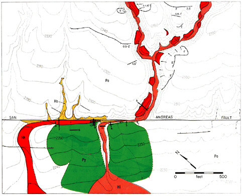
FIGURE 4.25 A detailed geologic map of Wallace Creek in the Carrizo Plain of central California. The 130- and 475-meter offsets of a stream channel (orange) and an alluvial fan apex (green) yield a Holocene slip rate for the San Andreas fault of 34 ± 3 millimeters per year. SOURCE: K. Sieh and R.H. Jahns, Holocene activity of the San Andreas fault at Wallace Creek, California, Geol. Soc. Am. Bull., 95, 883-896, 1984; see also <http://www.scec.org/wallacecreek/>.
greater depths is particularly powerful in delineating reverse faulting, and it has been used to delineate a major blind thrust beneath central Los Angeles (Figure 4.27). Future progress will likely come through “unified structural representations” that employ model-based methods and advanced visualization tools to integrate large sets of neotectonic, borehole, and seismic data, including tomographic images produced from natural earthquake sources (95).
Paleoseismology
Paleoseismology is the geological investigation of individual earthquakes decades, centuries, or millennia after their occurrence (96). Where-as neotectonics considers deformations summed over many episodes of
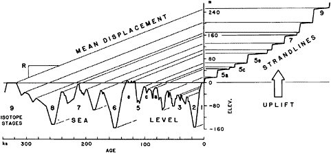
FIGURE 4.26 The rate of uplift of a series of marine terraces is commonly estimated by relating the elevation of the terraces to the history of sea-level fluctuations, which has been determined from analysis of oxygen isotope ratios in the minuscule shells of plankton accumulating on the ocean floor for hundreds of thousands of years. In this idealized drawing, the parallel, sloping lines represent the rate of uplift of the coastline. SOURCE: K.R. LaJoie, Coastal tectonics, in National Research Council, Active Tectonics, National Academy Press, Washington, D.C., 266 pp., 1986.
deformation, paleoseismology focuses on the geological record of specific events. Evidence reconstructed from sequences of large earthquakes spanning thousands of years is proving to be crucial to the general understanding of the size distribution of earthquakes, irregularities of the seismic process, and space-time patterns of fault slippage. By virtue of its extension through many earthquake cycles, paleoseismology provides some of the best information for long-term forecasting of major earthquakes on individual faults and for investigating the nature of the earthquake cycle. Paleoseismic features are associated with three types of processes:
-
disarticulation at a fault rupture, including fault scarps, wedges of debris at their base, fissures, and disarticulated strata of various origins;
-
changes in sea level or disruption of fluvial gradients, including ponded sediment and deformed fluvial and marine terraces; and
-
secondary effects of earthquake rupture, including manifestations of strong ground shaking such as mass wasting (landslides, rockfalls, and turbidites), liquefaction phenomena (sand blows, clastic dikes, seismites, lateral spreads), and tsunami deposits.
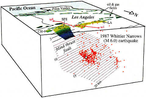
FIGURE 4.27 Southwest-looking perspective of the Puente Hills blind thrust fault (contoured in kilometers), which ruptured to produce the M 6 Whittier Narrows earthquake of 1987 (white dot). Relocated aftershocks (red dots) delineated a north-dipping plane, and seismic reflection surveys (colored contours) showed that this fault extends toward the surface beneath the active Puente Hills anticline. SOURCE: J.H. Shaw and P. Shearer, Southern California Earthquake Center.
Fault Rupture Many important active faults ruptured most recently in prehistoric or pre-instrumental time. In the case of southern California’s great 1857 earthquake, the approximate length of the rupture could be deduced from written accounts of shaking, but the actual slip as a function of distance along the San Andreas fault was determined only by measurement of offset landforms more than a century after the event (97); these measurements implied a moment magnitude of about 7.9. Incrementally larger offsets suggested that prior events were similar in size (98). Other examples include ruptures along faults in New Zealand and Alaska, the North Anatolian fault, and the Fuyun fault (99). The erosion of dated scarps in extensional regimes, such as the Basin and Range Province of the western United States (100), permits determination of the sequence of ruptures along normal faults. Numerous paleoseismic investigations have used colluvial wedges as evidence of prehistoric ruptures. These features are preserved along dip-slip faults.
Paleoseismic Sea-Level and Fluvial Grade Changes Geomorphic and stratigraphic evidence for changes in sea level often indicate paleoseismic uplift or submergence of a coastline, and flights of small coastal terraces commonly indicate a series of prehistoric seismic uplifts. The extent and magnitude of uplift allow estimation of the source parameters of the underlying rupture plane. Deformed river beds, such as the Mississippi, also provide constraints on the source parameters of seismic faults and, in combination with fault-bend fold modeling, reveal the nature of the events, here one of the great 1811-1812 sequences (101).
Sudden submergence associated with large earthquakes of the Cascadian subduction zone and overlying faults appears in estuarine stratigraphy along the coastlines of Oregon, Washington, and British Columbia (102). Discovery of these records helped to change the widely held view that subduction in the Pacific Northwest was principally aseismic.
Restriction of the upward growth of coral by exposure during low tides (103) offers high resolution of records of submergence and uplift. This technique has been used to estimate the source parameters for the giant (M 8.9-9.2) Sumatran subduction event of 1833 (104).
Seismically induced landslides, rockfalls, and submarine turbidity flows are well documented, as are seismically induced liquefaction phenomena (105). The widespread occurrence of rockfalls and landslides, shown by lichenometry to be of similar age, may indicate paleo-earthquakes in parts of New Zealand (106). The age of submarine turbidite deposits off the coast of Washington and Oregon suggests that they were dislodged during large Cascadian subduction-zone earthquakes (107).
Ancient liquefaction features in the central United States reveal not only that the region of the 1811-1812 New Madrid earthquakes has suffered prior large earthquakes about every 600 years, but also that the Wabash Valley and other midcontinent regions are susceptible to damaging earthquakes (108). Paleoliquefaction gives evidence that events such as the M 7 Charleston earthquake have stricken the South Carolina region about every 1500 years (109). Deformed lake beds of the Dead Sea not only provide a record of strong shaking, but also show that ruptures cluster into 10,000-year sequences separated by similarly lengthy periods of quiescence (110).
4.4 FAULT AND ROCK MECHANICS
In the context of earthquake science, the study of fault and rock mechanics aims to describe the macroscopic phenomena of fault slip and rock deformation in terms of the microscopic transport processes that operate on crystalline and atomic scales. This discipline lies at the core of earthquake studies because it connects the phenomenology of fault-
system science to the reductionist approach of condensed-matter physics. Its activities are focused in two observational environments:
-
laboratory research to characterize the properties of rocks and faults under the pressure, temperature, chemical, and strain-rate conditions that operate during the earthquake cycle—such observations are basic ingredients for the investigation of earthquake processes and the formulation of mechanistic and phenomenological models of rock friction; and
-
field research to elucidate the structure and processes of real fault zones, accounting for differences in rock types and tectonic regimes— these observations provide information on the tectonic stresses that drive lithospheric deformation and on the scaling of laboratory-based models to the parameter range of tectonic earthquakes.
The gap between laboratory scales of centimeters and field scales of kilometers has been a major stumbling block. Valuable information has come from rock-deformation and seismicity measurements in controlled environments such as boreholes and deep mines (see below), but bridging this gap relies heavily on fault-system modeling, the principal subject of Chapter 5.
Laboratory Studies of Rock Deformation
Quantifying the stress-strain response is conducted primarily in the laboratory, where rock samples are deformed in high-stress testing machines under controlled-state conditions. The sizes of the samples are small, ranging from a centimeter or less to a meter at most (111).
Rock Friction The modern study of fault friction began in the mid-1960s, when William Brace and his coworkers at the Massachusetts Institute of Technology first investigated stick-slip behavior as a mechanical model of earthquakes through a series of laboratory experiments. They recognized that stick-slip faulting depends on how the friction changes when slip conditions, particularly the sliding velocity, are modified. The introduction of servo-controlled testing machines in 1970, and the subsequent development of high-precision, double-direct-shear and rotary-shear devices (112), allowed detailed measurements of friction to be made for a wide range of materials under variable sliding conditions. This work, described in Section 2.5, led to the formulation of rate- and state-dependent friction relations (Box 4.4; Figure 4.28).
The micromechanical understanding of friction is incomplete and remains the subject of active laboratory research (113) as well as theoretical studies involving computer simulations of granular media (Figure 4.29).
Nevertheless, the rate-state description has enjoyed considerable success as a phenomenological theory of fault friction (114). It has unified the concepts of static and dynamic friction into a time-dependent theory of frictional evolution, furnished realistic constitutive equations for modeling earthquakes as stick-slip instabilities (115), and provided a mechanical basis for describing the key aspects of earthquake nucleation, including earthquake productivity as a function of stress (116) and precursory sliding. The size of the nucleation zone generating the precursory sliding is proportional to the critical slip distance Dc, so that the small laboratory values of Dc—less than a few hundred microns for gouge thicknesses up to 3 millimeters (117)—imply that the nucleation process will typically involves slip on a fault patch with a radius less than a few tens of meters, equivalent to only a magnitude-zero earthquake. The smallness of this aseismic moment release may explain why precursory slip has evaded detection on surface strainmeters (118).
Rate-dependent models of friction also furnish the framework for understanding the depth distribution of shallow earthquakes. In the notation of Box 4.4, the increase in friction with (steady-state) slipping velocity is equal to the difference between the coefficients a and b, so that the friction is velocity strengthening where a – b > 0 and velocity weakening where a – b < 0. The latter condition is necessary to nucleate dynamic faulting. How the difference a – b depends on pressure, temperature, and composition can be investigated in the laboratory. The thickness of the seismogenic zone can usually be ascribed to an upper cutoff associated with velocity strengthening in a shallow layer of poorly consolidated rocks and sediments and a lower cutoff caused by a temperature-dominated increase in a – b with depth (Figure 4.30).
Ductile Flow In addition to its effect on friction, raising temperature enhances the mobility of dislocations, allowing plastic behavior to occur at lower stresses, while elevating pressure suppresses the nucleation and growth of cracks by increasing the normal stresses across crack surfaces. Consequently, at some depth, called the brittle-ductile transition, rock deformation takes place entirely by ductile flow (119). The way in which jerky fault motions couple to this steadier, deeper flow is a complex issue, requiring detailed information about rock rheology below the seismogenic zone. For example, according to the model in Figure 4.30, crustal seismicity should stop at depths shallower than the brittle-ductile transition, which implies that the lithosphere is stronger than predicted by the early laboratory-based models, which pegged the brittle-ductile transition to the base of the seismic zone.
Detailed measurements of deformation mechanisms in rocks indicate that several deformation mechanisms contribute to the transition from
|
BOX 4.4 Rate- and State-Dependent Friction In one type of rock-friction experiment, a sample is cut to introduce a fault surface and subjected to a constant normal stress sn across this surface. The load point in a very stiff testing apparatus is first driven at constant velocity V0 until the friction on the fault surface obtains a steady-state value µ0 = t0/sn, where t0 is the shear stress. As in the case of static strength, this “base friction” is observed to depend only weakly on lithology and temperature.1 The velocity is then increased to V, and the change in µ is monitored. Many materials—rocks of various types, fault gouge, glass, paper, some metals and plastics, even wood (see Figure 4.28)—exhibit a characteristic response in which the friction first jumps quickly to a new value a ln (V/V0) and then decays more or less exponentially by an amount b ln (V/V0) over the distance Dc. The critical slip distance Dc varies from 2 to 100 microns and increases with surface roughness; for experiments where the fault zone contains gouge, it also increases with the particle size and thickness of the gouge. This behavior is described by a rate-state friction equation: µ = µ0 + a ln(V/V0) + b ln(V0?/Dc). In this expression, ? is a state variable with the dimensions of time, which satisfies a first-order differential equation of the form d?/dt = F(V?/Dc), where F(1) = 0. The latter condition implies that in steady state (d?/dt = 0), the state variable becomes ?ss = Dc/V and the friction attains the value µss = µ0 + (a – b) ln(V/V0). Therefore, the sign of a – b determines whether the friction associated with a velocity increase evolves to a higher value (a – b > 0: velocity strengthening) or a lower value (a – b < 0: velocity weakening). The stability of a fault to slow loading depends on this steady-state rheology and not on the details of F. Velocity weakening is required for stick-slip instabilities, and they occur in less stiff apparatus than imagined here. The temporal behavior of the friction is determined by the details of the evolution-rate function F = d?/dt, and several forms are in common use. The version of the constitutive relation originally put forward by Dieterich2 corresponds to An alternative proposed by Ruina3 is Both provide adequate descriptions of the velocity-step experiments, but there are important differences in their behaviors. As the slip velocity drops to zero, the evo |
|
lution rate vanishes in Ruina’s version, whereas it goes to unity in Dieterich’s. Hence, the Ruina form requires that slip occur to change friction, and is thus called a “slip law,” while the Dieterich form is a “slowness law” that allows faults to strengthen during periods of stationary contact. Various analyses have been made to assess the relative merits of these evolution laws in fitting laboratory data4 or simulating the transient behaviors of real faults. As C. Marone noted in a recent review, however, “distinguishing between them in the laboratory, even at room temperatures, has proven difficult … the distinction is subtle and often unresolvable owing to noise and other trends in the data.” Alternate forms of the evolution function have also been investigated,5 and the rate-state equations have been generalized to include more than one state variable6 and changes in normal stress sn.7 |
brittle behavior at shallow levels to fully plastic flow at great depths. Tensional microcracking, frictional sliding, and other nominally brittle mechanisms persist over a range of conditions where the sample shows macroscopically ductile behavior. The rheology of rocks in this “semibrittle” field differs from the predictions of flow laws measured at higher temperatures. In particular, semibrittle behavior is characterized by dilatancy and a greater dependence of strength on pressure (120). Combining the laboratory data on brittle, semibrittle, and ductile behavior of rocks with temperature profiles, compositional models, and scaling laws provides estimates of the rheological structure of the lithosphere that can be tested with field observations of deformation (121).
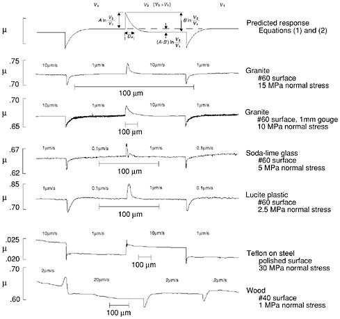
FIGURE 4.28 Results of laboratory experiments showing a similar frictional response for a variety of surfaces, including rock, glass, plastic, steel, and wood. Coefficient of friction m is plotted for stepwise changes in slipping velocity V. The upper panel is the predicted response for the slowness version of the rate- and state-dependent friction law, described in Box 4.4. The similarity indicates the wide applicability of this formalism. SOURCE: J.H. Dieterich and B. Kilgore, Direct observation of frictional contacts: New insights for state-dependent properties, Pure Appl. Geophys.,143, 283-302, 1994.
Field Studies of Faulting
Rock masses involved in faulting have large-scale structural features (joints, gouge zones, and compositional boundaries) that make their behavior different from the rock materials tested in the laboratory. Data gathered in the field are therefore essential in establishing the applicability of laboratory models and determining scaling relationships for the key constitutive parameters.
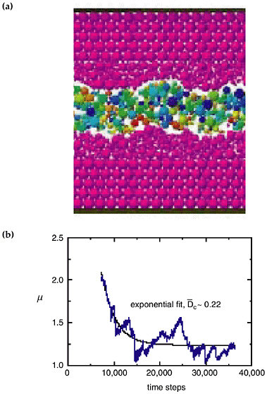
FIGURE 4.29 (a) Two-dimensional lattice solid model of fault gouge between two rough surfaces used in numerical simulations of frictional behavior. (b) Decay of macroscopic friction averaged over several slide-hold-slide cycles computed for this model (blue curve), and an exponential fit to obtain the critical slip distance Dc (black curve). SOURCE: S. Abe, J.H. Dieterich, P. Mora, and D. Place, Simulation of the influence of rate- and state-dependent friction on the macroscopic behavior of complex fault zones with the lattice solid model, Pure Appl. Geophys.,159, 1967-1983, 2002.
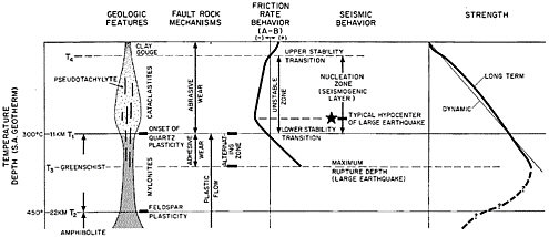
FIGURE 4.30 Hypothetical model of a major continental strike-slip fault such as the San Andreas, showing (from left to right) the depth variation of geologic features, deformation mechanisms, friction rate parameter a – b, seismic behavior, and strength (fault yield stress). Earthquakes can nucleate in the unstable zone where a – b is negative, implying friction that weakens with increasing sliding velocity. SOURCE: C.H. Scholz, The Mechanics of Earthquakes and Faulting, Cambridge University Press, Cambridge, U.K., p. 129, 1990. Reprinted with the permission of Cambridge University Press.
Fault Mechanics Cracks occur in three primary modes: mode-I tensile cracks where the displacement is normal to the plane of the crack, mode-II cracks where displacements are parallel to the crack plane and normal to the crack edge, and mode-III cracks where displacements are parallel to the crack plane and the crack edge. A fundamental problem, identified in the 1970s, is that simple mode-II shear cracks, which resemble faults, cannot propagate in their own plane owing to the stress concentrations at the crack tip (122). Detailed studies over the next decade demonstrated that shear cracks propagate by forming tensile cracks at their tips to relieve the local stress concentrations (123). The extension of these tensile cracks then plays a fundamental role in linking up parallel mode-II cracks in an en echelon stair-step pattern, concentrating shear stresses on the plane of the mode-II crack. Geologic observations indicate that fault formation processes are broadly similar. For example, there is a well-defined correlation between the total width of a fault zone (i.e., the width of the en echelon shear faults) and the total displacement on a fault (124). For individual faults, there is similar correlation due to the formation of gouge along the fault plane (125). Observations of the structures, displacements, and mineralogy within large granitic bodies have provided strong evidence for the coupled growth of mode-I and mode-II cracks in the nucleation and formation of large-scale shear faults (126).
On a larger scale, the field analysis of fault structures furnishes information on the apparent coefficient of friction governing fault strength. As deformation progresses within a fault system, crustal blocks undergo rotations and the faults bounding these blocks become misoriented with respect to the regional stress system, eventually causing them to “lock up” at a critical angle to the maximum compressive stress (127). Under the assumption that the sliding surfaces have zero cohesive strength (i.e., their strength is proportional to the normal stress), the critical angles can be used to estimate the coefficient of friction. Low-displacement faults in a variety of tectonic regimes typically give values consistent with Byerlee’s law: µ = 0.6-0.85 (128). The notable exceptions are shallow-dipping extensional detachment faults and major transform faults like the San Andreas, which are anomalously weak and may require some mechanism to maintain fluid overpressures.
Fault-Zone Petrology Field-scale observations provide important constraints on the genesis of fine-grained rocks in fault zones (129). C. Lapworth first described highly deformed rocks, which he called mylonites (literally, “milled rock”), in the Moine thrust of northwestern Scotland, but it was not until the latter part of the 20th century that geologists recognized that recrystallization and plastic flow can cause the fine grain sizes found in these high-temperature rocks (130). Fine-grained fault rocks are now generally classified
according to the two principal deformation mechanisms that produce them (131): cataclastites (including gouge and ultracataclastites), resulting from elastofrictional processes, and mylonites (including ultramylonites and pseudotachylytes), resulting from crystal-plastic flow, including pressure solution, melting, and other diffusion-aided processes. In most fault rocks, there is textural evidence for variations in the combination and competition of processes particularly for seismogenic faults that experience cycling of deformation rates over many orders of magnitude. Nonetheless, there is a general sequence progressing from cataclasites in the brittle seismogenic zone to mylonites in the ductile lower crust (132). Mylonite zones associated with exhumed faults can reach widths of 4 kilometers (133).
At shallow depths, fault zones range from a fraction of a meter to hundreds of meters in width. At depths less than 5 kilometers, large-displacement faults of the San Andreas system appear to consist of one to several very narrow slip zones, each less than a few centimeters in width, embedded in cataclastically deformed regions several meters thick; these shear structures lie within damage zones up to several hundred meters thick (134). The damage zones are regions of enhanced permeability and reduced elastic moduli (135); they exhibit a high degree of alteration and comprise small faults, fractures, and veins typically oriented at high angles to the main fault, which indicates that most of the damage zone accommodates little net slip (136).
The energetics of seismic slip is a critical issue (137). The elastic energy released when a fault slips is converted primarily into heat (138), which gives rise to two thermomechanical effects: transient heat pulses associated with individual earthquakes and an elevation in the steady-state heat flow near the fault zone resulting from many such events. Evidence for the former is seen in exhumed fault-zone rocks called pseudotachylytes that show evidence of partial melting during mylonitization (139). Evidence for the latter comes from metamorphic aureoles around faults (140). In the case of the Alpine fault of New Zealand, rocks deformed in strike-slip faulting have been uplifted from midcrustal depths to the surface by more recent oblique thrusting. The potassium-argon ages of Mesozoic schists exposed along the fault zone decrease from 150 million years ago to 0 million years ago as the fault zone is approached, which has been interpreted as a loss of radiogenic argon caused by frictional heating. The average shear stresses required to produce this heating are on the order of 50 megapascals (141). Similar values have been obtained to explain the origin of anatectic granites in the Main Central Thrust of the Himalayas by fault-zone heating (142). These large frictional stresses are at odds with the surface heat-flow measurements along the San Andreas fault, which show no significant anomaly due to strain heating (see Section 2.5).
Stress Observations and Modeling
Earthquakes happen when the local shear stress on a fault plane increases beyond its frictional strength. Considerable progress has been made in mapping the large-scale lateral variations in the stress field, as well as in understanding the variations in lithospheric strength as a function of depth. Three important conclusions have been drawn:
-
Stress orientations are uniform over large (about 500- to 1000-kilometer) distances and consistent with the source of stress being the same forces that drive motions of the lithospheric plates (Figure 3.22).
-
Strength within the upper crust is well approximated by Byerlee’s law, with considerable evidence pointing to a ductile zone of low strength in the lower continental crust in geographic regions where the crust is thick or hot.
-
Earthquakes occur at localized zones of low strength, not localized zones of higher stress.
Methods for Estimating Stress Stress orientations can be mapped using a number of stress-field indicators that sample the stress regime of the upper crust. The geological indicators include fault slip data (143) and volcanic vent alignments (144). The geophysical indicators include earthquake focal mechanisms, as well as several techniques based on measurements made in deep boreholes: wellbore breakouts, hydraulic fracturing, and overcoring. Each technique is based on certain assumptions which, if unsatisfied, can lead to bias. For example, the pressure (P) and tension (T) axes determined from earthquake focal mechanisms are commonly taken to be indicators of the maximum and minimum axes of tectonic stress, but in realistic situations where the slip occurs on some preexisting fault surface or other plane of weakness (e.g., a sedimentary bedding plane), individual focal mechanisms can deviate up to 40 degrees from the principal stress directions, which accounts for much of the scatter seen among earthquakes occurring in the same tectonic stress regime (145). If enough data are available and the fabric bias is not too strong, simple averaging over this scatter usually gives reliable results (146). A more formal procedure is to invert sets of focal mechanism solutions from a given region for the most self-consistent set of principal stress axes (147).
The stress magnitude is considerably more difficult to estimate than the stress orientation. The analysis of earthquake radiation provides the stress drops but not the absolute stresses during faulting, and there has been considerable debate about the absolute stresses acting on major faults such as the San Andreas based on indirect indicators such as heat flow and fault-zone petrology (see Section 2.5). The best estimates of local
stress magnitude and orientation come from borehole experiments that use hydrofracturing techniques. Inflatable rubber packers are used to isolate a section of a vertical borehole, which is then pressurized with fluids until a tensile fracture is induced. If one of the principal stresses is vertical, a vertical fracture will form at the azimuth of the greatest horizontal principal stress. With knowledge of the pressure-time history of the borehole, the magnitude of the stress can be calculated (148).
Borehole Measurements and Experiments
Almost all extant data on earthquake processes have been collected in the laboratory or from surface-based measurements. A number of key quantities, such as fluid pressures, cannot be directly measured or accurately inferred from surface measurements alone (149). For example, it is difficult to assess the importance of fluids in earthquake generation and rupture based solely on studies of exhumed fault zones, because the complex history of uplift and denudation severely alters, or even destroys, the evidence on deformation mechanisms, fault-zone mineralogy, and fluid compositions during the actual faulting. Drilling holes to relatively shallow seismogenic depths (less than 5 kilometers) is feasible, however, and the means have been developed to sample fault-zone materials and pore fluids, to make a variety of down-hole measurements, and to conduct in situ experiments related to the physics of faulting. Several nations, particularly Germany, have mounted ambitious programs to explore the physical properties and mechanical state of the Earth’s crust through deep drilling (150). Fault-zone drilling has received high priority in several recent scientific drilling programmatic assessments, both on continents and in the oceans (151).
Drilling into active fault zones, whether in the ocean basins or on continents, presents a number of technological and programmatic challenges. Nevertheless, measurements in the Kontinentale Tiefbohrprogramm (KTB) borehole in Germany have provided critical in situ data on crustal processes and the physics of faulting. Moreover, drilling projects to depths of 4 kilometers, such as that proposed for SAFOD at Parkfield, California, have the potential to provide the types of data on fault-zone composition, structure, mechanical behavior, and physical properties that are needed to address the question of why plate-bounding faults are anomalously weak.
NOTES
|
8. |
U.S. Geological Survey, Requirements for an Advanced National Seismic System, U.S. Geological Survey Circular 1188, Denver, Colo., 56 pp., 1999. This report lists 41 regional networks comprising 3095 earthquake-monitoring stations that are operated by the USGS, research universities, state geological surveys, private companies, and other organizations throughout the United States. |
|
9. |
A major program to densify regional networks in seismically active regions was launched by the USGS in the late 1960s (J.P. Eaton, W.H.K. Lee, and L.C. Pakiser, Microearthquakes and mechanics of earthquake generation, San Andreas fault, Tectonophysics, 9, 259-282, 1970). The principal goal was the accurate location of small earthquakes to delineate fault structures and measure changes in low-level seismicity that might be precursory to larger earthquakes; therefore, emphasis was placed on recording the arrival times of initial P waves using very sensitive, high-frequency instruments with precise timing control. |
|
10. |
National Research Council, Assessing the Nation’s Earthquakes: The Health and Future of Regional Seismic Networks, National Academy Press, Washington, D.C., 67 pp., 1990. That report emphatically recommended that “the federal government should establish a more rational, coordinated, and stable means of support for the seismic networks of the United States.” Several important steps have been taken toward improving and coordinating seismic monitoring efforts at the regional level. Two coordinating bodies have been formed: the Council of the National Seismic System, comprising primarily the operators of conventional weak-motion monitoring networks (<http://www.cnss.org>), and the Consortium of Organizations for Strong Motion Observational Systems, whose membership mostly includes strong-motion network operators. |
|
11. |
The piezoelectric transducers used in mine monitoring have usable response to 7 kilohertz and are recorded at rates of up to 10,000 samples per second. Local networks comprising these sensors can locate events of magnitudes below –2 in rock volumes with linear dimensions of 1 kilometer. |
|
12. |
E. Richardson and T.H. Jordan, Seismicity in deep gold mines of South Africa: Implications for tectonic earthquakes, Bull. Seis. Soc. Am., 92, 1766-1782, 2002. |
|
13. |
W.H. Bakun and A.G. Lindh, The Parkfield, California prediction experiment, Earthq. Predict. Res. 3, 285-304, 1985. In addition to the USGS, participating institutions include the University of California, Berkeley; Lawrence Berkeley National Laboratory; University of California, Riverside; University of Wisconsin; Rensselaer Polytechnic Institute; University of California, San Diego; and Australia’s Commonwealth Scientific and Industrial Research Organization (CSIRO) Exploration and Mining. |
|
14. |
A. Michelini and T.V. McEvilly, Seismological studies at Parkfield: 1. Simultaneous inversion for velocity structure and hypocenters using B-splines parameterization, Bull. Seis. Soc. Am., 81, 524-552, 1991. |
|
15. |
For example, C.G. Sammis, R.M. Nadeau, and L.R. Johnson, How strong is an asperity? J. Geophys. Res., 104, 10,609-10,619, 1999. |
|
16. |
For example, E.D. Karageorgi, T.V. McEvilly, and R. Clymer, Seismological studies at Parkfield, IV. Variations in controlled-source waveform parameters and their correlation with seismicity, 1987-1994, Bull. Seis. Soc. Am., 87, 39-49, 1997. |
|
17. |
R.M. Nadeau and T.V. McEvilly, Fault slip rates at depth from recurrence intervals of repeating microearthquakes, Science, 285, 718-1138, 1999. |
|
18. |
R.M. Nadeau and L.R. Johnson, Seismological studies at Parkfield, VI. Moment release rates and estimates of source parameters for small repeating earthquakes, Bull. Seis. Soc. Am., 88, 790-814, 1998. |
|
19. |
W.L. Ellsworth, M.V. Matthews, R.M. Nadeau, S.P. Nishenko, P.A. Reasenberg, and R.W. Simpson, A physically-based earthquake recurrence model for estimation of long-term earthquake probabilities, Workshop on Earthquake Recurrence: State of the Art and Directions for the Future, Instituto Nazionale de Geofisica, Rome, February 22-25, 1999. |
|
20. |
A national network was recommended, for example, in National Research Council, U.S. Earthquake Observatories: Recommendations for a New National Network, National Academy Press, Washington, D.C., 122 pp., 1980. |
|
21. |
The National Strong-Motion Network operated by the USGS currently involves 900 accelerographs at 628 stations in 32 states and the Caribbean (see <http://nsmp.wr.usgs.gov>). |
|
22. |
The PEER database is unique in distributing strong-motion data that have been processed to remove instrument response and noise and integrated for velocity and displacement using a standard algorithm, which makes the data especially suitable for engineering applications (see <http://peer.berkeley.edu/smcat>). |
|
23. |
National Research Council, Recommendations for the Strong-Motion Program in the United States, National Academy Press, Washington, D.C., 59 pp., 1987. |
|
24. |
|
|
25. |
The PASSCAL pool comprises a variety of instrument types and configurations, including more than 400 portable, seismic instruments. IRIS manages a PASSCAL instrument center at New Mexico Tech in Socorro, New Mexico, which provides software and logistical support to scientists in the design and execution of their experiments. RAMP instruments can be shipped anywhere in the world in less than 24 hours. See <http://www.iris.edu/passcal/passcal.htm>. |
|
26. |
The USGS maintains a pool of about 100 portable digital seismographs in Menlo Park, California, and Golden, Colorado, for aftershock studies, and it also operates portable seismographs in urban arrays (e.g., San Jose, California; Seattle, Washington) to record small and moderate earthquakes that can be analyzed to determine site response and basin effects at frequencies of 0.1 to 20 hertz. These deployments have proven that even weak ground motions from nearby M 2 earthquakes can be recorded successfully in high-noise urban environments. |
|
27. |
Simplifications are often made in parameterizing Earth structure. For example, high-frequency seismic waves are relatively insensitive to independent variations in the mass density ? except at reflecting interfaces; attenuation in pure compression can usually be ignored relative to attenuation in shear, and low-frequency waves are relatively insensitive to small-scale variations in the shear attenuation factor. On the other hand, the wave velocities in some regions of the Earth can be moderately anisotropic (i.e., they depend on the direction of wave propagation, as well as position), which requires the introduction of additional elastic parameters. |
|
28. |
The NEIS telemeters data from the GSN, USNSN, and other networks, locating approximately 15,000 earthquakes annually, and publishes data on these events in a variety of formats. The Quick Epicenter Determinations, a very preliminary list of earthquakes, is computed daily and is available via the Internet. The Preliminary Determination of Epicenters (PDE) is published and distributed weekly to those contributing data to the NEIS. The PDE, Monthly Listing is published monthly and is also available over the Internet. The Earthquake Data Report, also a monthly publication, provides additional and more detailed information for the use of seismologists on a data exchange basis. Other publications include CD-ROMs, maps, and an annual book United States Earthquakes. |
|
29. |
The ISC was formed in Edinburgh in 1964 to continue the work of the British Geological Survey in producing the International Seismological Summary (described in Section 2.3). In 1970, with the help of the United Nations Educational, Scientific and Cultural Organization and other international scientific bodies, the center was reconstituted as an international nongovernmental body, funded by interested institutions in about 7 countries; today nearly 50 countries fund the ISC. The ISC analysis of earthquake data is under-taken in monthly batches and begins after 22 months to allow the information used to be as complete as possible; the final product, the Bulletin of the International Seismological Centre, is published routinely about two years after the data are collected. |
|
|
nia: An alternative interpretation, Science, 210, 534-536, 1981; W.E. Strange, The impact of refraction correction on leveling interpretations in southern California, J. Geophys. Res., 86, 2809-2834, 1981; R.S. Stein, Role of elevation-dependent errors on the accuracy of geodetic leveling in the southern California uplift, 1953-1979, in Earthquake Prediction—An International Review, D.W. Simpson and P.G. Richards, eds., American Geophysical Union, Maurice Ewing Series, 4, Washington, D.C., pp. 441-456, 1981). |
|
39. |
Errors in leveling lines accumulate as a constant times the square root of the line length L. The constant of proportionality is typically 3 millimeters when L is expressed in kilometers, such that for L = 25 kilometers, the standard error is about 15 millimeters. Measurement precision with GPS is about 1 to 2 millimeters in horizontal position and 5 to 10 millimeters in vertical position, which can be achieved over short length scales for observation periods of a few hours and at length scales of hundreds of kilometers with day-long observations. Thus, several years of continuous GPS recording can yield steady-state velocity estimates with a precision of under 1 millimeter per year. The precision of such long-term measurements depends critically on stable, deeply anchored monuments. |
|
40. |
T.A. Herring, I.I. Shapiro, T.A. Clark, C. Ma, J.W. Ryan, B.R. Schupler, C.A. Knight, G. Lundqvist, D.B. Shaffer, N.R. Vandenberg, B.E. Corey, H.F. Hinteregger, A.E.E. Rogers, J.C. Webber, A.R. Whitney, G. Elgered, B.O. Ronnang, and J.L. Davis, Geodesy by radio interferometry: Evidence for contemporary plate motion, J. Geophys. Res., 91, 8341-8347, 1986; T.H. Jordan and J.B. Minster, Measuring crustal deformation in the American West, Sci. Am., 256, 48-58, 1988. |
|
41. |
The utility of GPS for a variety of military, commercial, and recreational purposes has reduced the price of navigation-quality receivers with resolutions of about 10 meters to a few hundred dollars. However, geodetic-quality receivers that operate off the GPS carrier phase are an order of magnitude more expensive, partly because they require better electronics and must process two frequencies to correct for signal delays caused by charged particles in the Earth’s ionosphere. Errors in GPS data come from errors in the reference frame, drift of the clocks onboard the satellites, refraction in the ionosphere and troposphere, multipath reflection of radio waves from the satellites, and so forth. These error sources can be included as terms in the basic equations to model GPS signals, and with sufficiently redundant data, the errors can be reduced dramatically. Large continuous networks are especially valuable for this purpose. In tectonic geodesy an additional error arises from nontectonic motions of the survey points caused by soil motions and fluid withdrawal in the region of the survey point. To reduce site instability, the Southern California Continuous GPS Network has developed an effective type of monument fixed at four points, each more than 10 meters below ground, by stainless steel rods welded to the surface monument. |
|
42. |
K. Feigl, D. Agnew, Y. Bock, D. Dong, A. Donnellan, B. Hager, T. Herring, D. Jackson, T. Jordan, R. King, S. Larsen, K Larson, M. Murray, Z. Shen, and F. Webb, Space geodetic measurement of crustal deformation in central and Southern California, 1984-1992, J. Geophys. Res., 98, 21,677-21,712, 1993. |
|
43. |
The International GPS Service for Geodynamics (IGS) integrates several forms of geodetic measurement to provide precise estimates of the satellite orbital parameters, the locations of selected tracking stations, and other important information needed in GPS processing. For more information, see <http://igscb.jpl.nasa.gov/>. |
|
44. |
Because of the need to integrate information into a global network, GPS data processing and interpretation depend critically on data sharing. The International GPS Services for Geodynamics, the Universities NAVSTAR Consortium, and the Southern California Earthquake Center, among many organizations, have made great progress in publishing GPS data freely over the Internet, contributing greatly to scientific progress in tectonic geodesy. |
|
45. |
The first InSAR image of an earthquake displacement field was published by D. Massonnet, M. Rossi, C. Carmona, F. Adragna, G. Peltzer, K. Feigl, and T. Rabaute (The displacement field of the Landers earthquake mapped by radar interferometry, Nature, 364, 138-142, 1993), who used a series of radar images acquired by the European Remote Sensing (ERS) satellites to construct an interferogram of the 1992 Landers earthquake (M 7.3). |
|
46. |
G. Peltzer, P. Rosen, F. Rogez, and K. Hudnut, Postseismic rebound in fault stepovers caused by pore fluid flow, Science, 273, 1202-1204, 1996. |
|
47. |
The proposed ECHO mission would be carried out jointly between NASA, NSF, and the USGS to provide spatially continuous strain measurements over wide geographic areas. The design goals of the proposed InSAR mission are dense spatial (100 meters) and temporal (every eight days) coverage of the entire North American-Pacific plate boundary with vector solutions accurate to 2 millimeters on spatial scales of 50 kilometers over all terrain types, which exceeds the capabilities of existing and planned international SAR missions. Spatially continuous, but intermittent, InSAR images complement continuous GPS point measurements and will therefore contribute to the EarthScope science objectives. |
|
48. |
Stable aseismic slip was discovered at the Cienega Winery, which straddles the San Andreas fault south of Hollister, California (K.V. Steinbrugge, E.G. Zacher, D. Tocher, C.A. Whitten, and C.N. Clair, Creep on the San Andreas fault [California]—Analysis of geodetic measurements along the San Andreas fault, Bull. Seis. Soc. Am., 50, 396-404, 1960). The walls of the winery building have been progressively offset at a rate of 11 millimeters per year since it was built in 1948. This “creeping section” of the San Andreas extends 160 kilometers from San Juan Bautista to Parkfield, California. |
|
49. |
Near-fault tectonic geodesy is reviewed by A.G. Sylvester in National Research Council, Active Tectonics, National Academy Press, Washington, D.C., pp. 164-180, 1986. |
|
50. |
C.R. Allen, M. Wyss, J.N. Brune, A. Grantz, and R.E. Wallace, Displacements on the Imperial, Superstition Hills, and San Andreas faults triggered by the Borrego Mountain earthquake, U.S. Geological Survey Professional Paper 787, Reston, Va., pp. 87-104, 1972; S.S. Schulz, G. Mavco, R.O. Burford, and W.D. Smith, Long-term fault creep observations in central California, J. Geophys. Res., 87, 6977-6982, 1982; R.O. Burford, The response of creeping parts of the San Andreas fault to earthquakes on nearby faults; Two examples, Pure Appl. Geophys., 126, 499-529, 1988; C.H. Thurber, Creep events preceding small to moderate earthquakes on the San Andreas fault, Nature, 380, 425-428, 1996. |
|
51. |
D.C. Agnew, Strainmeters and tiltmeters, Rev. Geophys., 24, 579-624, 1986. |
|
52. |
I.S. Sacks, S. Suyehiro, A.T. Linde, and J.A. Snoke, Slow earthquakes and stress redistribution, Nature, 275, 599-602, 1978; A.T. Linde, S. Suyehiro, I. Miura, I.S. Sacks, and A. Takagi, Episodic aseismic earthquake precursors, Nature, 334, 513-515, 1988; M.T. Gladwin, High-precision multicomponent borehole deformation monitoring, Rev. Sci. Instr., 55, 2011-2016, 1984. |
|
53. |
PBO Steering Committee, The Plate Boundary Observatory: Creating a four-dimensional image of the deformation of western North America, White paper providing the scientific rationale and deployment strategy for a Plate Boundary Observatory based on a workshop held October 3-5, 1999. Available at <http://www.earthscope.org>. |
|
54. |
The Southern California Earthquake Center employed this strategy in its 1995 earthquake hazard estimate. See Working Group on California Earthquake Probabilities, Seismic hazards in southern California: Probable earthquake 1994 to 2024, Bull. Seis. Soc. Am., 85, 379-439, 1995. In combination with geologic estimates of fault slip rate, they used GPS estimates from K. Feigl, D. Agnew, Y. Bock, D. Dong, A. Donnellan, B. Hager, T. Herring, D. Jackson, T. Jordan, R. King, S. Larsen, K Larson, M. Murray, Z. Shen, and F. Webb, Space geodetic measurement of crustal deformation in Central and Southern California, 1984-1992, J. Geophys. Res., 98, 21,677-21,712, 1993. |
|
|
Sacks, Modeling of postseismic relaxation following the great 1857 earthquake, Southern California, Bull. Seis. Soc. Am.,82, 454-480, 1992; F.F. Pollitz and I.S. Sacks, Consequences of stress changes following the 1891 Nobi earthquake, Japan, Bull. Seis. Soc. Am., 85, 796-807, 1995; F. Press and C. Allen, Patterns of seismic release in the southern California region,J. Geophys. Res., 100, 6421-6430, 1995. |
|
75. |
The best bounds on the sizes of strain precursors are from recent earthquakes in California and Japan. See M.L.S. Johnson, A.T. Linde, and M.T. Gladwin (Near-field high resolution strain measurements prior to the October 18, 1989 Loma Prieta Ms 7.1 earthquake, Geophys. Res. Lett., 17, 1777-1780, 1990) for the Loma Prieta earthquake, and F.K. Wyatt, D.C. Agnew, and M. Gladwin (Continuous measurements of crustal deformation for the 1992 Landers earthquake sequence, Bull. Seis. Soc. Am., 84, 768-779, 1994) for the Landers earthquake. |
|
76. |
Developments in this field are summarized in the textbook The Geology of Earthquakes, by R.S. Yeats, K. Sieh, and C.R. Allen (Oxford University Press, Oxford, U.K., 568 pp., 1997). |
|
77. |
National Research Council, Active Tectonics, National Academy Press, Washington, D.C., 266 pp., 1986. |
|
78. |
The SRTM mission and results are described at <http://jpl.nasa.gov/srtm>. |
|
79. |
An example is the Airborne Topographic Mapper, mounted on an Otter aircraft and used in the U.S. Topographic Change Mapping Project, a joint venture among NOAA, NASA, and USGS; see <http://www.csc.noaa.gov/crs/tcm/>. |
|
80. |
In deep water (3 kilometers), oceanographic swath-mapping systems yield bathymetric maps with a horizontal resolution of about 60 meters and a vertical precision of a few meters. The resolution and precision improve more or less linearly with decreasing water depth. |
|
81. |
For example, N.N. Ambraseys and C.P. Melville, A History of Persian Earthquakes, Cambridge University Press, Cambridge, U.K., 219 pp., 1982; Y. Sugiyama, Neotectonics of southwest Japan due to the right-oblique subduction of the Philippine Sea plate, Geof. Int., 33, 53-76, 1994; D.C. Agnew and K. Sieh, A documentary study of the felt effects of the great California earthquake of 1857, Bull. Seis. Soc. Am., 68, 1717-1729, 1978; K. Satake, K. Shimazaki, Y. Tsuji, and K. Ueda, Time and size of a giant earthquake in Cascadia inferred from Japanese tsunami records of January 1700, Nature,379, 246-249, 1996. |
|
82. |
See R. Page, Dating episodes of faulting from tree rings: Effects of the 1958 rupture of the Fairweather fault on tree growth, Geol. Soc. Am. Bull., 81, 3085-3094, 1970; V.C. LaMarche, Jr. and R.E. Wallace, Evaluation of effects of trees on past movements on the San Andreas fault, northern California, Geol. Soc. Am. Bull., 83, 2665-2676, 1972; G.C. Jacoby, P.R. Sheppard, and K.E. Sieh, Irregular recurrence of large earthquakes along the San Andreas fault; Evidence from trees, Science, 241, 196-199, 1988; D.K. Yamaguchi, B.F. Atwater, D.E. Bunker, B.E. Benson, and M.S. Reid, Tree-ring dating the 1700 Cascadia earthquake, Nature, 389, 922-923, 1997. |
|
83. |
The age range, resolution, and applications of different techniques for dating surficial materials are described in J.S. Noller, J.M. Sowers, and W.R. Lettis, Quaternary Geochronology: Methods and Applications, American Geophysical Union, Washington, D.C., 582 pp., 2000. |
|
84. |
J.A. Spotila, K.A. Farley, and K. Sieh, Uplift and erosion of the San Bernardino Mountains associated with transpression along the San Andreas fault, California, as constrained by radiogenic helium thermochronometry, Tectonics,17, 360-378, 1998; C.R. Bacon, M.A. Lanphere, and D.E. Champion, Late Quaternary slip rate and seismic hazards of the West Klamath Lake fault zone near Crater Lake, Oregon Cascades, Geology, 27, 43-46, 1999; J. Lee, C.M. Rubin, and A. Calvert, Quaternary faulting history along the Deep Springs fault, California, Geol. Soc. Am. Bull., 113, 855-869, 2001; A.K. Jain, D. Kumar; S. Singh, A. |
|
|
Kumar, and N. Lal, Timing, quantification and tectonic modelling of Pliocene-Quaternary movements in the NW Himalaya; Evidence from fission track dating, Earth Planet. Sci. Lett., 179, 437-451, 2000; B.J. Szabo and J.N. Rosholt, Uranium-series nuclides in the Golden fault, Colorado, U.S.A.: Dating latest fault displacement and measuring recent uptake of radionuclides by fault-zone materials, Appl. Geochem., 4, 177-182, 1989. |
|
85. |
For example, K.E. Sieh, Prehistoric large earthquakes produced by slip on the San Andreas fault at Pallet Creek, California, J. Geophys. Res., 83, 3907-3939, 1978; K. Sieh, M. Stuiver, and D. Brillinger, A more precise chronology of earthquakes produced by the San Andreas fault in southern California, J. Geophys. Res., 94, 603-623, 1989. See Box 4.5. |
|
86. |
E. Bard, B. Hamelin, R.G. Fairbanks, and A. Zindler, Calibration of the 14C timescale over the past 30,000 years using mass spectrometric U-Th ages from Barbados corals, Nature, 345, 405-410, 1990. |
|
87. |
F.W. Taylor, C. Frohlich, J. Lecolle, and M. Strecker, Analysis of partially emerged corals and reef terraces in the central Vanuatu arc: Comparison of contemporary coseismic and nonseismic with Quaternary vertical movements, J. Geophys. Res., 92, 4905-4933, 1987; J. Zachariasen, K. Sieh, F. Taylor, R.L. Edwards, and W.S. Hantoro, Submergence and uplift associated with the giant 1833 Sumatran subduction earthquake: Evidence from coral microatolls, J. Geophys. Res., 104, 895-919, 1999. |
|
88. |
L.A. Perg, R.S. Anderson, and R.C. Finkel, Use of a new 10Be and 26Al inventory method to date marine terraces, Santa Cruz, California, USA, Geology, 29, 879-882, 2001; J. Van der Woerd, F.J. Ryerson, P. Tapponnier, Y. Gaudemer, R. Finkel, A.S. Meriaux, M. Caffee, G. Zhao, and Q. He, Holocene left-slip rate determined by cosmogenic surface dating on the Xidatan segment of the Kunlun fault (Qinghai, China), Geology, 26, 695-698, 1998; L.C. Benedetti, R.C. Finkel, G.C.P. King, R. Armijo, D. Papanastassiou, F.J. Ryerson, F. Flerit, and D. Farber, Earthquake time-slip history of the Kaparelli fault (Greece) from in situ chlorine-36 cosmogenic dating, EOS Trans. Am. Geophys. Union, 82, F931, 2001. |
|
89. |
Examples include neotectonic maps of Japan (Y. Kinugasa, E. Tsukada, and H. Yamazaki, Neotectonic map of Japan, Geological Atlas of Japan, 2nd ed., Asakura Publishing Company, Ltd., Tokyo, sheet 5, 1992), Turkey (F. Saroglu, O. Emre, and I. Kuscu, The east Anatolian fault zone of Turkey, Annales Tectonicae, Suppl. 6 (Special Issue), 99-125, 1992), Alaska (G. Plafker, L.M. Gilpin, and J.C. Lahr, Neotectonic map of Alaska, in The Geology of Alaska, G.B. Plafker and H. Berg, eds., Decade of North American Geology, G-1, Geological Society of America, Boulder, Colo., pl. 12 (map), 1994), southern Tibet (R. Armijo, P. Tapponnier, J.L. Mercier, and T.-L. Han, Quaternary extension in southern Tibet: Field observations and tectonic implications, J. Geophys. Res., 91, 13,803-13,872, 1986), and Sumatra (K. Sieh and D. Natawidjaja, Neotectonics of the Sumatran fault, J. Geophys. Res., 105, 28,295-28,336, 2000). |
|
90. |
The World Map of Major Active Faults being compiled under Project II-2 of the International Lithosphere Program is a step in this direction; see<http://www.gfzpotsdam.de/pb4/ilp96/projects.htm>. |
|
91. |
L.A. Reinen, J.D. Weeks, and T.E. Tullis, The frictional behavior of serpentinite: Implications for aseismic creep on shallow crustal faults, Geophys. Res. Lett., 18, 1921-1924, 1991; The frictional behavior of lizardite and antigorite serpentinites: Experiments, constitutive models, and implications for natural faults, Pure Appl. Geophys., 143, 317-358, 1994. |
|
92. |
J. Van der Woerd, F.J. Ryerson, P. Tapponnier, A.-S. Meriaux, Y. Gaudemer, B. Meyer, R.C. Finkel, M.W. Caffee, Z. Guoguang, and X. Zhiqin, Uniform slip-rate across the Kunlun fault: Implications for seismic behavior and large-scale tectonics, Geophys. Res. Lett., 27, 2353-2356, 2000. |
|
93. |
J.-C. Lee, Y.-G. Chen, K. Sieh, K. Mueller, W.-S. Chen, H.-T. Chu, Y.-C. Chan, C. Rubin, and R. Yeats, A vertical exposure of the 1999 surface rupture of the Chelungpu fault at Wufeng, western Taiwan: Structural and paleoseismic implications for an active thrust fault, Bull. Seis. Soc. Am., 91, 914-929, 2001. |
|
94. |
R.S. Yeats, Large-scale Quaternary detachments in Ventura basin, southern California, J. Geophys. Res., 88, 569-583, 1983. |
|
95. |
Developing a unified structural representation for southern California has been set as a high-priority goal of the Southern California Earthquake Center; see Southern California Earthquake Center, Science Plan for 2002-2007, University of Southern Calif., 9 pp., 2001, available at <http://www.scec.org/aboutSCEC/documents/science.plan.2002/>. |
|
96. |
This definition of paleoseismology is offered in the historical overview by R.S. Yeats and C.S. Prentice, Introduction to special session: Paleoseismology, J. Geophys. Res., 101, 5847-5853, 1996. A survey of the subject is given by J.P. McCalpin, ed., Paleoseismology, International Geophysics Series 62, Academic Press, San Diego, Calif., 588 pp., 1996. |
|
97. |
D.C. Agnew and K. Sieh, A documentary study of the felt effects of the great California earthquake of 1857, Bull. Seis. Soc. Am., 68, 1717-1729, 1978. Geologic features corresponding to individual earthquake offsets on the San Andreas, including the 1857 event, were first recognized by R.E. Wallace (Notes on stream channels offset by the San Andreas fault, southern Coast Ranges, California, in Proceedings of a Conference on Geological Problems of the San Andreas Fault System, W.R. Dickinson and A. Grantz, eds., Stanford University Publications in Geological Science 11, Stanford, Calif., pp. 6-21, 1968). |
|
98. |
K. Sieh, M. Stuvier, and D. Brillinger, A more precise chronology of earthquakes produced by the San Andreas fault in southern California, J. Geophys. Res., 94, 603-623, 1989. |
|
99. |
See K.R. Berryman, S. Beanland, A. Cooper, H. Cutten, R. Norris, and P. Wood, The Alpine fault, New Zealand: Variation in Quaternary structural style and geomorphic expression, Annales Tectonicae, Suppl. 6 (Special Issue), 126-163, 1992; K. Sieh, A review of geological evidence for recurrence times of large earthquakes, in Earthquake Prediction—An International Review, D. Simpson and P. Richards, eds., American Geophysical Union, Maurice Ewing Series 4, Washington, D.C., pp. 181-207, 1981; A.A. Barka, Slip distribution along the North Anatolian fault associated with the large earthquakes of 1939-1967, Bull. Seis. Soc. Am., 86, 1238-1254, 1996; Q.-D. Deng and P.-Z. Zhang, Research on the geometry of shear fracture zones, J. Geophys. Res., 89, 5699-5710, 1984. |
|
100. |
R.E. Wallace, Profiles and ages of young fault scarps, north-central Nevada, Geol. Soc. Am. Bull., 88, 1267-1281, 1977. |
|
101. |
K. Mueller, J. Champion, M. Guccione, and K. Kelson, Fault slip rates in the modern New Madrid seismic zone, Science, 286, 1135-1138, 1999. |
|
102. |
J. Clague, Evidence for large earthquakes at the Cascadia subduction zone, Rev. Geophys., 35, 439-460, 1997. |
|
103. |
F.W. Taylor, C. Frohlich, J. Lecolle, and M. Strecker, Analysis of partially emerged corals and reef terraces in the central Vanuatu arc: Comparison of contemporary coseismic and nonseismic with Quaternary vertical movements, J. Geophys. Res., 92, 4905-4933, 1987; R.L. Edwards, F.W. Taylor, and G.J. Wasserburg, Dating earthquakes with high-precision thorium-230 ages of very young corals, Earth Planet. Sci. Lett., 90, 371-381, 1988. |
|
104. |
J. Zachariasen, K. Sieh, F. Taylor, R.L. Edwards, and W.S. Hantoro, Submergence and uplift associated with the giant 1833 Sumatran subduction earthquake: Evidence from coral microatolls, J. Geophys. Res., 104, 895-919, 1999; K. Sieh, S. Ward, D. Natawidjaja, and B. Suwargadi, Crustal deformation at the Sumatran subduction zone revealed by coral rings, Geophys. Res. Lett., 26, 3141-3144, 1999. |
|
105. |
See R.S. Yeats, K. Sieh, and C.R. Allen, The Geology of Earthquakes, Oxford University Press, Oxford, U.K., 568 pp., 1997, for a more extensive enumeration and discussion. |
|
106. |
W.B. Bull, J. King, F. Kong, T. Moutoux, and W.M. Phillips, Lichen dating of coseismic landslide hazards in alpine mountains, Geomorph., 10, 253-264, 1994. |
|
107. |
J. Adams, Paleoseismicity of the Cascadia subduction zone: Evidence from turbidites off the Oregon-Washington margin, Tectonics, 9, 569-583, 1990. |


